stat341 / CM 361

Computational Statistics and Data Analysis is a course offered at the University of Waterloo
Spring 2009
Instructor: Ali Ghodsi

Sampling (Generating random numbers)

Generating Random Numbers - May 12, 2009

Generating random numbers in a computational setting presents challenges. A good way to generate random numbers in computational statistics involves analyzing various distributions using computational methods. As a result, the probability distribution of each possible number appears to be uniform (pseudo-random). Outside a computational setting, presenting a uniform distribution is fairly easy (for example, rolling a fair die repetitively to produce a series of random numbers from 1 to 6).

We begin by considering the simplest case: the uniform distribution.

Multiplicative Congruential Method

One way to generate pseudo random numbers from the uniform distribution is using the Multiplicative Congruential Method. This involves three integer parameters a, b, and m, and a seed variable x₀. This method deterministically generates a sequence of numbers (based on the seed) with a seemingly random distribution (with some caveats). It proceeds as follows:

[math]\displaystyle{ x_{i+1} = (ax_{i} + b) \mod{m} }[/math]

For example, with a = 13, b = 0, m = 31, x₀ = 1, we have:

[math]\displaystyle{ x_{i+1} = 13x_{i} \mod{31} }[/math]

So,

[math]\displaystyle{ \begin{align} x_{0} &{}= 1 \end{align} }[/math]

[math]\displaystyle{ \begin{align} x_{1} &{}= 13 \times 1 + 0 \mod{31} = 13 \\ \end{align} }[/math]

[math]\displaystyle{ \begin{align} x_{2} &{}= 13 \times 13 + 0 \mod{31} = 14 \\ \end{align} }[/math]

[math]\displaystyle{ \begin{align} x_{3} &{}= 13 \times 14 + 0 \mod{31} =27 \\ \end{align} }[/math]

etc.

The above generator of pseudorandom numbers is called a Mixed Congruential Generator or Linear Congruential Generator, as they involve both an additive and a muliplicative term. For correctly chosen values of a, b, and m, this method will generate a sequence of integers including all integers between 0 and m - 1. Scaling the output by dividing the terms of the resulting sequence by m - 1, we create a sequence of numbers between 0 and 1, which is similar to sampling from a uniform distribution.

Of course, not all values of a, b, and m will behave in this way, and will not be suitable for use in generating pseudo random numbers.

For example, with a = 3, b = 2, m = 4, x₀ = 1, we have:

[math]\displaystyle{ x_{i+1} = (3x_{i} + 2) \mod{4} }[/math]

So,

[math]\displaystyle{ \begin{align} x_{0} &{}= 1 \end{align} }[/math]

[math]\displaystyle{ \begin{align} x_{1} &{}= 3 \times 1 + 2 \mod{4} = 1 \\ \end{align} }[/math]

[math]\displaystyle{ \begin{align} x_{2} &{}= 3 \times 1 + 2 \mod{4} = 1 \\ \end{align} }[/math]

etc.

For an ideal situation, we want m to be a very large prime number, [math]\displaystyle{ x_{n}\not= 0 }[/math] for any n, and the period is equal to m-1. In practice, it has been found by a paper published in 1988 by Park and Miller, that a = 7⁵, b = 0, and m = 2³¹ - 1 = 2147483647 (the maximum size of a signed integer in a 32-bit system) are good values for the Multiplicative Congruential Method.

Java's Random class is based on a generator with a = 25214903917, b = 11, and m = 2⁴⁸<ref>http://java.sun.com/javase/6/docs/api/java/util/Random.html#next(int)</ref>. The class returns at most 32 leading bits from each x_i, so it is possible to get the same value twice in a row, (when x₀ = 18698324575379, for instance) without repeating it forever.

General Methods

Since the Multiplicative Congruential Method can only be used for the uniform distribution, other methods must be developed in order to generate pseudo random numbers from other distributions.

Inverse Transform Method

This method uses the fact that when a random sample from the uniform distribution is applied to the inverse of a cumulative density function (cdf) of some distribution, the result is a random sample of that distribution. This is shown by this theorem:

Theorem:

If [math]\displaystyle{ U \sim~ \mathrm{Unif}[0, 1] }[/math] is a random variable and [math]\displaystyle{ X = F^{-1}(U) }[/math], where F is continuous, monotonic, and is the cumulative density function (cdf) for some distribution, then the distribution of the random variable X is given by F(X).

Proof:

Recall that, if f is the pdf corresponding to F, then,

[math]\displaystyle{ F(x) = P(X \leq x) = \int_{-\infty}^x f(x) }[/math]

[math]\displaystyle{ \int_1^{\infty} \frac{x^k}{x^2} dx }[/math]

So F is monotonically increasing, since the probability that X is less than a greater number must be greater than the probability that X is less than a lesser number.

Note also that in the uniform distribution on [0, 1], we have for all a within [0, 1], [math]\displaystyle{ P(U \leq a) = a }[/math].

So,

[math]\displaystyle{ \begin{align} P(F^{-1}(U) \leq x) &{}= P(F(F^{-1}(U)) \leq F(x)) \\ &{}= P(U \leq F(x)) \\ &{}= F(x) \end{align} }[/math]

Completing the proof.

Procedure (Continuous Case)

This method then gives us the following procedure for finding pseudo random numbers from a continuous distribution:

• Step 1: Draw [math]\displaystyle{ U \sim~ Unif [0, 1] }[/math].
• Step 2: Compute [math]\displaystyle{ X = F^{-1}(U) }[/math].

Example:

Suppose we want to draw a sample from [math]\displaystyle{ f(x) = \lambda e^{-\lambda x} }[/math] where [math]\displaystyle{ x \gt 0 }[/math] (the exponential distribution).

We need to first find [math]\displaystyle{ F(x) }[/math] and then its inverse, [math]\displaystyle{ F^{-1} }[/math].

[math]\displaystyle{ F(x) = \int^x_0 \theta e^{-\theta u} du = 1 - e^{-\theta x} }[/math]

[math]\displaystyle{ F^{-1}(x) = \frac{-\log(1-y)}{\theta} = \frac{-\log(u)}{\theta} }[/math]

Now we can generate our random sample [math]\displaystyle{ i=1\dots n }[/math] from [math]\displaystyle{ f(x) }[/math] by:

[math]\displaystyle{ 1)\ u_i \sim Unif[0, 1] }[/math]

[math]\displaystyle{ 2)\ x_i = \frac{-\log(u_i)}{\theta} }[/math]

The [math]\displaystyle{ x_i }[/math] are now a random sample from [math]\displaystyle{ f(x) }[/math].

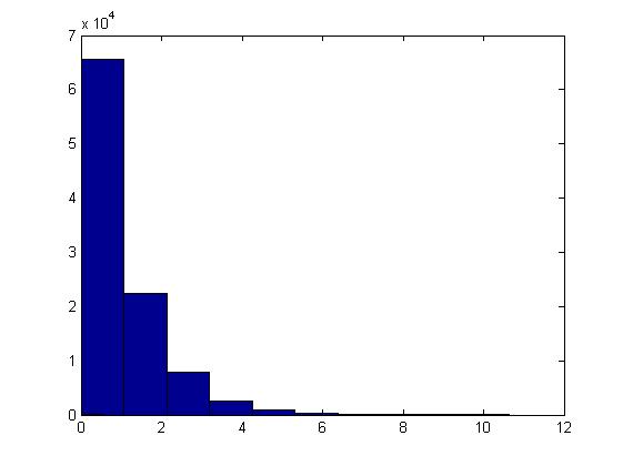
This example can be illustrated in Matlab using the code below. Generate [math]\displaystyle{ u_i }[/math], calculate [math]\displaystyle{ x_i }[/math] using the above formula and letting [math]\displaystyle{ \theta=1 }[/math], plot the histogram of [math]\displaystyle{ x_i }[/math]'s for [math]\displaystyle{ i=1,...,100,000 }[/math].

u=rand(1,100000);
x=-log(1-u)/1;
hist(x)

The histogram shows exponential pattern as expected.

The major problem with this approach is that we have to find [math]\displaystyle{ F^{-1} }[/math] and for many distributions it is too difficult (or impossible) to find the inverse of [math]\displaystyle{ F(x) }[/math]. Further, for some distributions it is not even possible to find [math]\displaystyle{ F(x) }[/math] (i.e. a closed form expression for the distribution function, or otherwise; even if the closed form expression exists, it's usually difficult to find [math]\displaystyle{ F^{-1} }[/math]).

Procedure (Discrete Case)

The above method can be easily adapted to work on discrete distributions as well.

In general in the discrete case, we have [math]\displaystyle{ x_0, \dots , x_n }[/math] where:

[math]\displaystyle{ \begin{align}P(X = x_i) &{}= p_i \end{align} }[/math]

[math]\displaystyle{ x_0 \leq x_1 \leq x_2 \dots \leq x_n }[/math]

[math]\displaystyle{ \sum p_i = 1 }[/math]

Thus we can define the following method to find pseudo random numbers in the discrete case (note that the less-than signs from class have been changed to less-than-or-equal-to signs by me, since otherwise the case of [math]\displaystyle{ U = 1 }[/math] is missed):

• Step 1: Draw [math]\displaystyle{ U~ \sim~ Unif [0,1] }[/math].
• Step 2:
  • If [math]\displaystyle{ U \lt p_0 }[/math], return [math]\displaystyle{ X = x_0 }[/math]
  • If [math]\displaystyle{ p_0 \leq U \lt p_0 + p_1 }[/math], return [math]\displaystyle{ X = x_1 }[/math]
  • ...
  • In general, if [math]\displaystyle{ p_0+ p_1 + \dots + p_{k-1} \leq U \lt p_0 + \dots + p_k }[/math], return [math]\displaystyle{ X = x_k }[/math]

Example (from class):

Suppose we have the following discrete distribution:

[math]\displaystyle{ \begin{align} P(X = 0) &{}= 0.3 \\ P(X = 1) &{}= 0.2 \\ P(X = 2) &{}= 0.5 \end{align} }[/math]

The cumulative density function (cdf) for this distribution is then:

[math]\displaystyle{ F(x) = \begin{cases} 0, & \text{if } x \lt 0 \\ 0.3, & \text{if } 0 \leq x \lt 1 \\ 0.5, & \text{if } 1 \leq x \lt 2 \\ 1, & \text{if } 2 \leq x \end{cases} }[/math]

Then we can generate numbers from this distribution like this, given [math]\displaystyle{ u_0, \dots, u_n }[/math] from [math]\displaystyle{ U \sim~ Unif[0, 1] }[/math]:

[math]\displaystyle{ x_i = \begin{cases} 0, & \text{if } u_i \leq 0.3 \\ 1, & \text{if } 0.3 \lt u_i \leq 0.5 \\ 2, & \text{if } 0.5 \lt u_i \leq 1 \end{cases} }[/math]

This example can be illustrated in Matlab using the code below:

p=[0.3,0.2,0.5];
for i=1:1000;
  u=rand;
  if u <= p(1)
    x(i)=0;
  elseif u < sum(p(1,2))
    x(i)=1;
  else
    x(i)=2;
  end
end

Acceptance-Rejection Sampling - May 14, 2009

Today, we continue the discussion on sampling (generating random numbers) from general distributions with the Acceptance/Rejection Method.

Acceptance/Rejection Method

Suppose we wish to sample from a target distribution [math]\displaystyle{ f(x) }[/math] that is difficult or impossible to sample from directly. Suppose also that we have a proposal distribution [math]\displaystyle{ g(x) }[/math] from which we have a reasonable method of sampling (e.g. the uniform distribution). Then, if there is a constant [math]\displaystyle{ c \ |\ c \cdot g(x) \geq f(x)\ \forall x }[/math], accepting samples drawn in successions from [math]\displaystyle{ c \cdot g(x) }[/math] with ratio [math]\displaystyle{ \frac {f(x)}{c \cdot g(x)} }[/math] close to 1 will yield a sample that follows the target distribution [math]\displaystyle{ f(x) }[/math]; on the other hand we would reject the samples if the ratio is not close to 1.

The following graph shows the pdf of [math]\displaystyle{ f(x) }[/math] (target distribution) and [math]\displaystyle{ c \cdot g(x) }[/math] (proposal distribution)

File:fxcgx.JPG

At x=7; sampling from [math]\displaystyle{ c \cdot g(x) }[/math] will yield a sample that follows the target distribution [math]\displaystyle{ f(x) }[/math]

At x=9; we will reject samples according to the ratio [math]\displaystyle{ \frac {f(x)}{c \cdot g(x)} }[/math] after sampling from [math]\displaystyle{ c \cdot g(x) }[/math]

Proof

Note the following:

• [math]\displaystyle{ Pr(X|accept) = \frac{Pr(accept|X) \times Pr(X)}{Pr(accept)} }[/math] (Bayes' theorem)
• [math]\displaystyle{ Pr(accept|X) = \frac{f(x)}{c \cdot g(x)} }[/math]
• [math]\displaystyle{ Pr(X) = g(x)\frac{}{} }[/math]

So, [math]\displaystyle{ Pr(accept) = \int^{}_x Pr(accept|X) \times Pr(X) dx }[/math] [math]\displaystyle{ = \int^{}_x \frac{f(x)}{c \cdot g(x)} g(x) dx }[/math] [math]\displaystyle{ = \frac{1}{c} \int^{}_x f(x) dx }[/math] [math]\displaystyle{ = \frac{1}{c} }[/math]

Therefore, [math]\displaystyle{ Pr(X|accept) = \frac{\frac{f(x)}{c\ \cdot g(x)} \times g(x)}{\frac{1}{c}} = f(x) }[/math] as required.

Procedure (Continuous Case)

• Choose [math]\displaystyle{ g(x) }[/math] (a density function that is simple to sample from)
• Find a constant c such that :[math]\displaystyle{ c \cdot g(x) \geq f(x) }[/math]

1. Let [math]\displaystyle{ Y \sim~ g(y) }[/math]
2. Let [math]\displaystyle{ U \sim~ Unif [0,1] }[/math]
3. If [math]\displaystyle{ U \leq \frac{f(x)}{c \cdot g(x)} }[/math] then X=Y; else reject and go to step 1

Example:

Suppose we want to sample from Beta(2,1), for [math]\displaystyle{ 0 \leq x \leq 1 }[/math]. Recall:

[math]\displaystyle{ Beta(2,1) = \frac{\Gamma (2+1)}{\Gamma (2) \Gamma(1)} \times x^1(1-x)^0 = \frac{2!}{1!0!} \times x = 2x }[/math]

• Choose [math]\displaystyle{ g(x) \sim~ Unif [0,1] }[/math]
• Find c: c = 2 (see notes below)

1. Let [math]\displaystyle{ Y \sim~ Unif [0,1] }[/math]
2. Let [math]\displaystyle{ U \sim~ Unif [0,1] }[/math]
3. If [math]\displaystyle{ U \leq \frac{2Y}{2} = Y }[/math], then X=Y; else go to step 1

[math]\displaystyle{ c }[/math] was chosen to be 2 in this example since [math]\displaystyle{ \max \left(\frac{f(x)}{g(x)}\right) }[/math] in this example is 2. This condition is important since it helps us in finding a suitable [math]\displaystyle{ c }[/math] to apply the Acceptance/Rejection Method.

In MATLAB, the code that demonstrates the result of this example is:

   j = 1;
       while i < 1000
           y = rand;
           u = rand;
           if u <= y
               x(j) = y;
               j = j + 1;
               i = i + 1;
           end
       end
       hist(x);
       

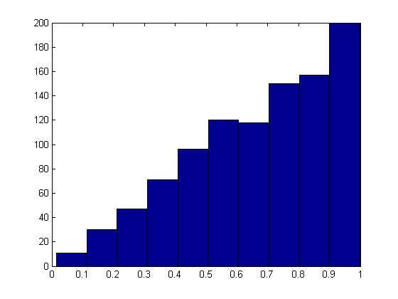
The histogram produced here should follow the target distribution, [math]\displaystyle{ f(x) = 2x }[/math], for the interval [math]\displaystyle{ 0 \leq x \leq 1 }[/math].

The histogram shows the PDF of a Beta(2,1) distribution as expected.

The Discrete Case

The Acceptance/Rejection Method can be extended for discrete target distributions. The difference compared to the continuous case is that the proposal distribution [math]\displaystyle{ g(x) }[/math] must also be discrete distribution. For our purposes, we can consider g(x) to be a discrete uniform distribution on the set of values that X may take on in the target distribution.

Example

Suppose we want to sample from a distribution with the following probability mass function (pmf):

P(X=1) = 0.15
P(X=2) = 0.55
P(X=3) = 0.20
P(X=4) = 0.10 

• Choose [math]\displaystyle{ g(x) }[/math] to be the discrete uniform distribution on the set [math]\displaystyle{ \{1,2,3,4\} }[/math]
• Find c: [math]\displaystyle{ c = \max \left(\frac{f(x)}{g(x)} \right)= 0.55/0.25 = 2.2 }[/math]

1. Generate [math]\displaystyle{ Y \sim~ Unif \{1,2,3,4\} }[/math]
2. Let [math]\displaystyle{ U \sim~ Unif [0,1] }[/math]
3. If [math]\displaystyle{ U \leq \frac{f(x)}{2.2 \times 0.25} }[/math], then X=Y; else go to step 1

Limitations

If the proposed distribution is very different from the target distribution, we may have to reject a large number of points before a good sample size of the target distribution can be established. It may also be difficult to find such [math]\displaystyle{ g(x) }[/math] that satisfies all the conditions of the procedure.

We will now begin to discuss sampling from specific distributions.

Special Technique for sampling from Gamma Distribution

Recall that the cdf of the Gamma distribution is:

[math]\displaystyle{ F(x) = \int_0^{\lambda x} \frac{e^{-y}y^{t-1}}{(t-1)!} dy }[/math]

If we wish to sample from this distribution, it will be difficult for both the Inverse Method (difficulty in computing the inverse function) and the Acceptance/Rejection Method.

Additive Property of Gamma Distribution

Recall that if [math]\displaystyle{ X_1, \dots, X_t }[/math] are independent exponential distributions with mean [math]\displaystyle{ \lambda }[/math] (in other words, [math]\displaystyle{ X_i\sim~ Exp (\lambda) }[/math]), then [math]\displaystyle{ \Sigma_{i=1}^t X_i \sim~ Gamma (t, \lambda) }[/math]

It appears that if we want to sample from the Gamma distribution, we can consider sampling from t independent exponential distributions with mean [math]\displaystyle{ \lambda }[/math] (using the Inverse Method) and add them up. Details will be discussed in the next lecture.

Techniques for Normal and Gamma Sampling - May 19, 2009

We have examined two general techniques for sampling from distributions. However, for certain distributions more practical methods exist. We will now look at two cases,
Gamma distributions and Normal distributions, where such practical methods exist.

Gamma Distribution

Given the additive property of the gamma distribution,

If [math]\displaystyle{ X_1, \dots, X_t }[/math] are independent random variables with [math]\displaystyle{ X_i\sim~ Exp (\lambda) }[/math] then,

[math]\displaystyle{ \Sigma_{i=1}^t X_i \sim~ Gamma (t, \lambda) }[/math]

We can use the Inverse Transform Method and sample from independent uniform distributions seen before to generate a sample following a Gamma distribution.

Procedure

1. Sample independently from a uniform distribution [math]\displaystyle{ t }[/math] times, giving [math]\displaystyle{ u_1,\dots,u_t }[/math]
2. Sample independently from an exponential distribution [math]\displaystyle{ t }[/math] times, giving [math]\displaystyle{ x_1,\dots,x_t }[/math] such that,
   [math]\displaystyle{ \begin{align} x_1 \sim~ Exp(\lambda)\\ \vdots \\ x_t \sim~ Exp(\lambda) \end{align} }[/math]
   
   Using the Inverse Transform Method,
   [math]\displaystyle{ \begin{align} x_i = -\frac {1}{\lambda}\log(u_i) \end{align} }[/math]
3. Using the additive property,
   [math]\displaystyle{ \begin{align} X &{}= x_1 + x_2 + \dots + x_t \\ X &{}= -\frac {1}{\lambda}\log(u_1) - \frac {1}{\lambda}\log(u_2) \dots - \frac {1}{\lambda}\log(u_t) \\ X &{}= -\frac {1}{\lambda}\log(\prod_{i=1}^{t}u_i) \sim~ Gamma (t, \lambda) \end{align} }[/math]

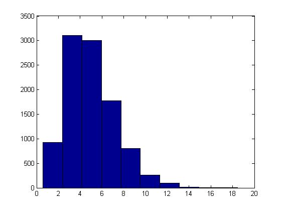
This procedure can be illustrated in Matlab using the code below with [math]\displaystyle{ t = 5, \lambda = 1 }[/math] :

U = rand(10000,5);
X = sum( -log(U), 2);
hist(X)

Normal Distribution

"Diagram of the Box Muller transform, which transforms uniformly distributed value pairs to normally distributed value pairs." [Box-Muller Transform, Wikipedia]

The cdf for the Standard Normal distribution is:

[math]\displaystyle{ F(Z) = \int_{-\infty}^{Z}\frac{1}{\sqrt{2\pi}}e^{-x^2/2}dx }[/math]

We can see that the normal distribution is difficult to sample from using the general methods seen so far, eg. the inverse is not easy to obtain from F(Z); we may be able to use the Acceptance-Rejection method, but there are still better ways to sample from a Standard Normal Distribution.

Box-Muller Method

[Add a picture WikiSysop 19:25, 1 June 2009 (UTC)]

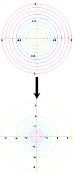
The Box-Muller or Polar method uses an approach where we have one space that is easy to sample in, and another with the desired distribution under a transformation. If we know such a transformation for the Standard Normal, then all we have to do is transform our easy sample and obtain a sample from the Standard Normal distribution.

Properties of Polar and Cartesian Coordinates

If x and y are points on the Cartesian plane, r is the length of the radius from a point in the polar plane to the pole, and θ is the angle formed with the polar axis then,

• [math]\displaystyle{ \begin{align} r^2 = x^2 + y^2 \end{align} }[/math]
• [math]\displaystyle{ \tan(\theta) = \frac{y}{x} }[/math]

• [math]\displaystyle{ \begin{align} x = r \cos(\theta) \end{align} }[/math]
• [math]\displaystyle{ \begin{align} y = r \sin(\theta) \end{align} }[/math]

Let X and Y be independent random variables with a standard normal distribution,

[math]\displaystyle{ X \sim~ N(0,1) }[/math]

[math]\displaystyle{ Y \sim~ N(0,1) }[/math]

also, let [math]\displaystyle{ r }[/math] and [math]\displaystyle{ \theta }[/math] be the polar coordinates of (x,y). Then the joint distribution of independent x and y is given by,

[math]\displaystyle{ \begin{align} f(x,y) = f(x)f(y) &{}= \frac{1}{\sqrt{2\pi}}e^{-\frac{x^2}{2}}\frac{1}{\sqrt{2\pi}}e^{-\frac{y^2}{2}} \\ &{}=\frac{1}{2\pi}e^{-\frac{x^2+y^2}{2}} \end{align} }[/math]

It can also be shown that the joint distribution of r and θ is given by,

[math]\displaystyle{ \begin{matrix} f(r,\theta) = \frac{1}{2}e^{-\frac{d}{2}}*\frac{1}{2\pi},\quad d = r^2 \end{matrix} }[/math]

Note that [math]\displaystyle{ \begin{matrix}f(r,\theta)\end{matrix} }[/math] consists of two density functions, Exponential and Uniform, so assuming that r and [math]\displaystyle{ \theta }[/math] are independent [math]\displaystyle{ \begin{matrix} \Rightarrow d \sim~ Exp(1/2), \theta \sim~ Unif[0,2\pi] \end{matrix} }[/math]

Procedure for using Box-Muller Method

1. Sample independently from a uniform distribution twice, giving [math]\displaystyle{ \begin{align} u_1,u_2 \sim~ \mathrm{Unif}(0, 1) \end{align} }[/math]
2. Generate polar coordinates using the exponential distribution of d and uniform distribution of θ,
   [math]\displaystyle{ \begin{align} d = -2\log(u_1),& \quad r = \sqrt{d} \\ & \quad \theta = 2\pi u_2 \end{align} }[/math]
3. Transform r and θ back to x and y,
   [math]\displaystyle{ \begin{align} x = r\cos(\theta) \\ y = r\sin(\theta) \end{align} }[/math]

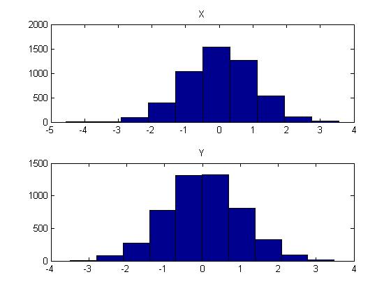
Notice that the Box-Muller Method generates a pair of independent Standard Normal distributions, x and y.

This procedure can be illustrated in Matlab using the code below:

u1 = rand(5000,1);
u2 = rand(5000,1);

d = -2*log(u1);
theta = 2*pi*u2;

x = d.^(1/2).*cos(theta);
y = d.^(1/2).*sin(theta);

figure(1);

subplot(2,1,1);
hist(x);
title('X');
subplot(2,1,2);
hist(y);
title('Y');

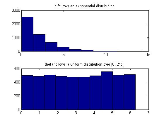
Also, we can confirm that d and theta are indeed exponential and uniform random variables, respectively, in Matlab by:

subplot(2,1,1);
hist(d);
title('d follows an exponential distribution');
subplot(2,1,2);
hist(theta);
title('theta follows a uniform distribution over [0, 2*pi]');

Useful Properties (Single and Multivariate)

Box-Muller can be used to sample a standard normal distribution. However, there are many properties of Normal distributions that allow us to use the samples from Box-Muller method to sample any Normal distribution in general.

Properties of Normal distributions

• [math]\displaystyle{ \begin{align} \text{If } & X = \mu + \sigma Z, & Z \sim~ N(0,1) \\ &\text{then } X \sim~ N(\mu,\sigma ^2) \end{align} }[/math]

• [math]\displaystyle{ \begin{align} \text{If } & \vec{Z} = (Z_1,\dots,Z_d)^T, & Z_1,\dots,Z_d \sim~ N(0,1) \\ &\text{then } \vec{Z} \sim~ N(\vec{0},I) \end{align} }[/math]

• [math]\displaystyle{ \begin{align} \text{If } & \vec{X} = \vec{\mu} + \Sigma^{1/2} \vec{Z}, & \vec{Z} \sim~ N(\vec{0},I) \\ &\text{then } \vec{X} \sim~ N(\vec{\mu},\Sigma) \end{align} }[/math]

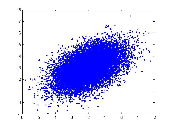
These properties can be illustrated through the following example in Matlab using the code below:

Example: For a Multivariate Normal distribution [math]\displaystyle{ u=\begin{bmatrix} -2 \\ 3 \end{bmatrix} }[/math] and [math]\displaystyle{ \Sigma=\begin{bmatrix} 1&0.5\\ 0.5&1\end{bmatrix} }[/math]

u = [-2; 3];
sigma = [ 1 1/2; 1/2 1];

r = randn(15000,2);
ss = chol(sigma);

X = ones(15000,1)*u' + r*ss;
plot(X(:,1),X(:,2), '.');

Note: In the example above, we had to generate the square root of [math]\displaystyle{ \Sigma }[/math] using the Cholesky decomposition,

ss = chol(sigma);

which gives [math]\displaystyle{ ss=\begin{bmatrix} 1&0.5\\ 0&0.8660\end{bmatrix} }[/math]. Matlab also has the sqrtm function:

ss = sqrtm(sigma);

which gives a different matrix, [math]\displaystyle{ ss=\begin{bmatrix} 0.9659&0.2588\\ 0.2588&0.9659\end{bmatrix} }[/math], but the plot looks about the same (X has the same distribution).

Monte Carlo Integration - May 26, 2009

Today's lecture completes the discussion on the Frequentists and Bayesian schools of thought and introduces Basic Monte Carlo Integration.

Frequentist vs Bayesian Example - Estimating Parameters

Estimating parameters of a univariate Gaussian:

Frequentist: [math]\displaystyle{ f(x|\theta)=\frac{1}{\sqrt{2\pi}\sigma}e^{-\frac{1}{2}*(\frac{x-\mu}{\sigma})^2} }[/math]
Bayesian: [math]\displaystyle{ f(\theta|x)=\frac{f(x|\theta)f(\theta)}{f(x)} }[/math]

Frequentist Approach

Let [math]\displaystyle{ X^N }[/math] denote [math]\displaystyle{ (x_1, x_2, ..., x_n) }[/math]. Using the Maximum Likelihood Estimation approach for estimating parameters we get:

[math]\displaystyle{ L(X^N; \theta) = \prod_{i=1}^N \frac{1}{\sqrt{2\pi}\sigma}e^{-\frac{1}{2}(\frac{x_i- \mu} {\sigma})^2} }[/math]

[math]\displaystyle{ l(X^N; \theta) = \sum_{i=1}^N -\frac{1}{2}log (2\pi) - log(\sigma) - \frac{1}{2} \left(\frac{x_i- \mu}{\sigma}\right)^2 }[/math]

[math]\displaystyle{ \frac{dl}{d\mu} = \displaystyle\sum_{i=1}^N(x_i-\mu) }[/math]

Setting [math]\displaystyle{ \frac{dl}{d\mu} = 0 }[/math] we get

[math]\displaystyle{ \displaystyle\sum_{i=1}^Nx_i = \displaystyle\sum_{i=1}^N\mu }[/math]

[math]\displaystyle{ \displaystyle\sum_{i=1}^Nx_i = N\mu \rightarrow \mu = \frac{1}{N}\displaystyle\sum_{i=1}^Nx_i }[/math]

Bayesian Approach

Assuming the prior is Gaussian:

[math]\displaystyle{ P(\theta) = \frac{1}{\sqrt{2\pi}\tau}e^{-\frac{1}{2}(\frac{x-\mu_0}{\tau})^2} }[/math]

[math]\displaystyle{ f(\theta|x) \propto \frac{1}{\sqrt{2\pi}\sigma}e^{-\frac{1}{2}(\frac{x_i-\mu}{\sigma})^2} * \frac{1}{\sqrt{2\pi}\tau}e^{-\frac{1}{2}(\frac{x-\mu_0}{\tau})^2} }[/math]

By completing the square we conclude that the posterior is Gaussian as well:

[math]\displaystyle{ f(\theta|x)=\frac{1}{\sqrt{2\pi}\tilde{\sigma}}e^{-\frac{1}{2}(\frac{x-\tilde{\mu}}{\tilde{\sigma}})^2} }[/math]

Where

[math]\displaystyle{ \tilde{\mu} = \frac{\frac{N}{\sigma^2}}{{\frac{N}{\sigma^2}}+\frac{1}{\tau^2}}\bar{x} + \frac{\frac{1}{\tau^2}}{{\frac{N}{\sigma^2}}+\frac{1}{\tau^2}}\mu_0 }[/math]

The expectation from the posterior is different from the MLE method. Note that [math]\displaystyle{ \displaystyle\lim_{N\to\infty}\tilde{\mu} = \bar{x} }[/math]. Also note that when [math]\displaystyle{ N = 0 }[/math] we get [math]\displaystyle{ \tilde{\mu} = \mu_0 }[/math].

Basic Monte Carlo Integration

Although it is almost impossible to find a precise definition of "Monte Carlo Method", the method is widely used and has numerous descriptions in articles and monographs. As an interesting fact, the term Monte Carlo is claimed to have been first used by Ulam and von Neumann as a Los Alamos code word for the stochastic simulations they applied to building better atomic bombs. Stochastic simulation refers to a random process in which its future evolution is described by probability distributions (counterpart to a deterministic process), and these simulation methods are known as Monte Carlo methods. [Stochastic process, Wikipedia]. The following example (external link) illustrates a Monte Carlo Calculation of Pi: [1]

We start with a simple example:

[math]\displaystyle{ I = \displaystyle\int_a^b h(x)\,dx }[/math]

[math]\displaystyle{ = \displaystyle\int_a^b w(x)f(x)\,dx }[/math]

where

[math]\displaystyle{ \displaystyle w(x) = h(x)(b-a) }[/math]

[math]\displaystyle{ f(x) = \frac{1}{b-a} \rightarrow }[/math] the p.d.f. is Unif[math]\displaystyle{ (a,b) }[/math]

[math]\displaystyle{ \hat{I} = E_f[w(x)] = \frac{1}{N}\displaystyle\sum_{i=1}^Nw(x_i) }[/math]

If [math]\displaystyle{ x_i \sim~ Unif(a,b) }[/math] then by the Law of Large Numbers [math]\displaystyle{ \frac{1}{N}\displaystyle\sum_{i=1}^Nw(x_i) \rightarrow \displaystyle\int w(x)f(x)\,dx = E_f[w(x)] }[/math]

Process

Given [math]\displaystyle{ I = \displaystyle\int^b_ah(x)\,dx }[/math]

1. [math]\displaystyle{ \begin{matrix} w(x) = h(x)(b-a)\end{matrix} }[/math]
2. [math]\displaystyle{ \begin{matrix} x_1, x_2, ..., x_n \sim UNIF(a,b)\end{matrix} }[/math]
3. [math]\displaystyle{ \hat{I} = \frac{1}{N}\displaystyle\sum_{i=1}^Nw(x_i) }[/math]

From this we can compute other statistics, such as

1. [math]\displaystyle{ SE=\frac{s}{\sqrt{N}} }[/math] where [math]\displaystyle{ s^2=\frac{\sum_{i=1}^{N}(Y_i-\hat{I})^2 }{N-1} }[/math] with [math]\displaystyle{ \begin{matrix}Y_i=w(x_i)\end{matrix} }[/math]
2. [math]\displaystyle{ \begin{matrix} 1-\alpha \end{matrix} }[/math] CI's can be estimated as [math]\displaystyle{ \hat{I}\pm Z_\frac{\alpha}{2}*SE }[/math]

Example 1

Find [math]\displaystyle{ E[\sqrt{x}] }[/math] for [math]\displaystyle{ \begin{matrix} f(x) = e^{-x}\end{matrix} }[/math]

1. We need to draw from [math]\displaystyle{ \begin{matrix} f(x) = e^{-x}\end{matrix} }[/math]
2. [math]\displaystyle{ \hat{I} = \frac{1}{N}\displaystyle\sum_{i=1}^Nw(x_i) }[/math]

This example can be illustrated in Matlab using the code below:

u=rand(100,1)
x=-log(u)
h= x.* .5
mean(h)
%The value obtained using the Monte Carlo method
F = @ (x) sqrt (x). * exp(-x)
quad(F,0,50)
%The value of the real function using Matlab

Example 2 Find [math]\displaystyle{ I = \displaystyle\int^1_0h(x)\,dx, h(x) = x^3 }[/math]

1. [math]\displaystyle{ \displaystyle I = x^4/4 = 1/4 }[/math]
2. [math]\displaystyle{ \displaystyle W(x) = x^3*(1-0) }[/math]
3. [math]\displaystyle{ Xi \sim~Unif(0,1) }[/math]
4. [math]\displaystyle{ \hat{I} = \frac{1}{N}\displaystyle\sum_{i=1}^N(x_i^3) }[/math]

This example can be illustrated in Matlab using the code below:

x = rand (1000)
mean(x^3)

Example 3 To estimate an infinite integral such as [math]\displaystyle{ I = \displaystyle\int^\infty_5 h(x)\,dx, h(x) = 3e^{-x} }[/math]

1. Substitute in [math]\displaystyle{ y=\frac{1}{x-5+1} =\gt dy=-\frac{1}{(x-4)^2}dx =\gt dy=-y^2dx }[/math]
2. [math]\displaystyle{ I = \displaystyle\int^1_0 \frac{3e^{-(\frac{1}{y}+4)}}{-y^2}\,dy }[/math]
3. [math]\displaystyle{ w(y) = \frac{3e^{-(\frac{1}{y}+4)}}{-y^2}(1-0) }[/math]
4. [math]\displaystyle{ Y_i \sim~Unif(0,1) }[/math]
5. [math]\displaystyle{ \hat{I} = \frac{1}{N}\displaystyle\sum_{i=1}^N(\frac{3e^{-(\frac{1}{y_i}+4)}}{-y_i^2}) }[/math]

Importance Sampling and Monte Carlo Simulation - May 28, 2009

During this lecture we covered two more examples of Monte Carlo simulation, finishing that topic, and begun talking about Importance Sampling.

Binomial Probability Monte Carlo Simulations

Example 1:

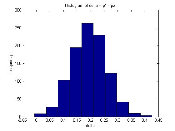
You are given two independent Binomial distributions with probabilities [math]\displaystyle{ \displaystyle p_1\text{, }p_2 }[/math]. Using a Monte Carlo simulation, approximate the value of [math]\displaystyle{ \displaystyle \delta }[/math], where [math]\displaystyle{ \displaystyle \delta = p_1 - p_2 }[/math].

[math]\displaystyle{ \displaystyle X \sim BIN(n, p_1) }[/math]; [math]\displaystyle{ \displaystyle Y \sim BIN(n, p_2) }[/math]; [math]\displaystyle{ \displaystyle \delta = p_1 - p_2 }[/math]

So [math]\displaystyle{ \displaystyle f(p_1, p_2 | x,y) = \frac{f(x, y|p_1, p_2)*f(p_1,p_2)}{f(x,y)} }[/math] where [math]\displaystyle{ \displaystyle f(x,y) }[/math] is a flat distribution and the expected value of [math]\displaystyle{ \displaystyle \delta }[/math] is as follows:

[math]\displaystyle{ \displaystyle \hat{\delta} = \int\int\delta f(p_1,p_2|X,Y)\,dp_1dp_2 }[/math]

Since X, Y are independent, we can split the conditional probability distribution:

[math]\displaystyle{ \displaystyle f(p_1,p_2|X,Y) \propto f(p_1|X)f(p_2|Y) }[/math]

We need to find conditional distribution functions for [math]\displaystyle{ \displaystyle p_1, p_2 }[/math] to draw samples from. In order to get a distribution for the probability 'p' of a Binomial, we have to divide the Binomial distribution by n. This new distribution has the same shape as the original, but is scaled. A Beta distribution is a suitable approximation. Let

[math]\displaystyle{ \displaystyle f(p_1 | X) \sim \text{Beta}(x+1, n-x+1) }[/math] and [math]\displaystyle{ \displaystyle f(p_2 | Y) \sim \text{Beta}(y+1, n-y+1) }[/math], where

[math]\displaystyle{ \displaystyle \text{Beta}(\alpha,\beta) = \frac{\Gamma(\alpha+\beta)}{\Gamma(\alpha)\Gamma(\beta)}p^{\alpha-1}(1-p)^{\beta-1} }[/math]

Process:

1. Draw samples for [math]\displaystyle{ \displaystyle p_1 }[/math] and [math]\displaystyle{ \displaystyle p_2 }[/math]: [math]\displaystyle{ \displaystyle (p_1,p_2)^{(1)} }[/math], [math]\displaystyle{ \displaystyle (p_1,p_2)^{(2)} }[/math], ..., [math]\displaystyle{ \displaystyle (p_1,p_2)^{(n)} }[/math];
2. Compute [math]\displaystyle{ \displaystyle \delta = p_1 - p_2 }[/math] in order to get n values for [math]\displaystyle{ \displaystyle \delta }[/math];
3. [math]\displaystyle{ \displaystyle \hat{\delta}=\frac{\displaystyle\sum_{\forall i}\delta^{(i)}}{N} }[/math].
   
   

Matlab Code:

The Matlab code for recreating the above example is as follows:

n=100; %number of trials for X
m=100; %number of trials for Y
x=80; %number of successes for X trials
y=60; %number of successes for y trials
p1=betarnd(x+1, n-x+1, 1, 1000);
p2=betarnd(y+1, m-y+1, 1, 1000);
delta=p1-p2;
mean(delta);

The mean in this example is given by 0.1938.

A 95% confidence interval for [math]\displaystyle{ \delta }[/math] is represented by the interval between the 2.5% and 97.5% quantiles which covers 95% of the probability distribution. In Matlab, this can be calculated as follows:

q1=quantile(delta,0.025);
q2=quantile(delta,0.975);

The interval is approximately [math]\displaystyle{ 95% CI \approx (0.06606, 0.32204) }[/math]

The histogram of delta is:

Note: In this case, we can also find [math]\displaystyle{ E(\delta) }[/math] analytically since [math]\displaystyle{ E(\delta) = E(p_1 - p_2) = E(p_1) - E(p_2) = \frac{x+1}{n+2} - \frac{y+1}{m+2} \approx 0.1961 }[/math]. Compare this with the maximum likelihood estimate for [math]\displaystyle{ \delta }[/math]: [math]\displaystyle{ \frac{x}{n} - \frac{y}{m} = 0.2 }[/math].

Example 2:

Bayesian Inference for Dose Response

We conduct an experiment by giving rats one of ten possible doses of a drug, where each subsequent dose is more lethal than the previous one:

[math]\displaystyle{ \displaystyle x_1\lt x_2\lt ...\lt x_{10} }[/math]

For each dose [math]\displaystyle{ \displaystyle x_i }[/math] we test n rats and observe [math]\displaystyle{ \displaystyle Y_i }[/math], the number of rats that survive. Therefore,

[math]\displaystyle{ \displaystyle Y_i \sim~ BIN(n, p_i) }[/math]
.

We can assume that the probability of death grows with the concentration of drug given, i.e. [math]\displaystyle{ \displaystyle p_1\lt p_2\lt ...\lt p_{10} }[/math]. Estimate the dose at which the animals have at least 50% chance of dying.

Let [math]\displaystyle{ \displaystyle \delta=x_j }[/math] where [math]\displaystyle{ \displaystyle j=min\{i|p_i\geq0.5\} }[/math]

We are interested in [math]\displaystyle{ \displaystyle \delta }[/math] since any higher concentrations are known to have a higher death rate.

Solving this analytically is difficult:

[math]\displaystyle{ \displaystyle \delta = g(p_1, p_2, ..., p_{10}) }[/math] where g is an unknown function

[math]\displaystyle{ \displaystyle \hat{\delta} = \int \int..\int_A \delta f(p_1,p_2,...,p_{10}|Y_1,Y_2,...,Y_{10})\,dp_1dp_2...dp_{10} }[/math]

where [math]\displaystyle{ \displaystyle A=\{(p_1,p_2,...,p_{10})|p_1\leq p_2\leq ...\leq p_{10} \} }[/math]

Process: Monte Carlo
We assume that

1. Draw [math]\displaystyle{ \displaystyle p_i \sim~ BETA(y_i+1, n-y_i+1) }[/math]
2. Keep sample only if it satisfies [math]\displaystyle{ \displaystyle p_1\leq p_2\leq ...\leq p_{10} }[/math], otherwise discard and try again.
3. Compute [math]\displaystyle{ \displaystyle \delta }[/math] by finding the first [math]\displaystyle{ \displaystyle p_i }[/math] sample with over 50% deaths.
4. Repeat process n times to get n estimates for [math]\displaystyle{ \displaystyle \delta_1, \delta_2, ..., \delta_N }[/math].
5. [math]\displaystyle{ \displaystyle \bar{\delta} = \frac{\displaystyle\sum_{\forall i} \delta_i}{N} }[/math].

For instance, for each dose level [math]\displaystyle{ X_i }[/math], for [math]\displaystyle{ 1\lt =i\lt =10 }[/math], 10 rats are used and it is observed that the numbers that are dying is [math]\displaystyle{ Y_i }[/math], where [math]\displaystyle{ Y_1 = 4, Y_2 = 3, }[/math]etc.

Importance Sampling

In statistics, Importance Sampling helps estimating the properties of a particular distribution. As in the case with the Acceptance/Rejection method, we choose a good distribution from which to simulate the given random variables. The main difference in importance sampling however, is that certain values of the input random variables in a simulation have more impact on the parameter being estimated than others. [Importance Sampling, Wikipedia] The following diagram illustrates a Monte Carlo approximation for g(x):

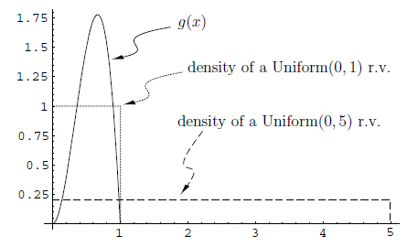
As the figure above shows, the uniform distribution [math]\displaystyle{ U\sim~Unif[0,1] }[/math] is a proposal distribution to sample from and g(x) is the target distribution. Here we cast the integral [math]\displaystyle{ \int_{0}^1 g(x)dx }[/math], as the expectation with respect to U such that [math]\displaystyle{ \int_{0}^1 g(x)= E(g(U)) }[/math]. Hence we can approximate by [math]\displaystyle{ \frac{1}{n}\displaystyle\sum_{i=1}^{n} g(u_i) }[/math].
[Source: Monte Carlo Methods and Importance Sampling, Eric C. Anderson (1999). Retrieved June 9th from URL: http://ib.berkeley.edu/labs/slatkin/eriq/classes/guest_lect/mc_lecture_notes.pdf]

In [math]\displaystyle{ I = \displaystyle\int h(x)f(x)\,dx }[/math], Monte Carlo simulation can be used only if it easy to sample from f(x). Otherwise, another method must be applied. If sampling from f(x) is difficult but there exists a probability distribution function g(x) which is easy to sample from, then [math]\displaystyle{ I }[/math] can be written as

[math]\displaystyle{ I = \displaystyle\int h(x)f(x)\,dx }[/math]

[math]\displaystyle{ = \displaystyle\int \frac{h(x)f(x)}{g(x)}g(x)\,dx }[/math]

[math]\displaystyle{ = \displaystyle E_g(w(x)) \rightarrow }[/math]the expectation of w(x) with respect to g(x) and therefore [math]\displaystyle{ \displaystyle x_1,x_2,...,x_N \sim~ g }[/math]

[math]\displaystyle{ = \frac{\displaystyle\sum_{i=1}^{N} w(x_i)}{N} }[/math] where [math]\displaystyle{ \displaystyle w(x) = \frac{h(x)f(x)}{g(x)} }[/math]

Process

1. Choose [math]\displaystyle{ \displaystyle g(x) }[/math] such that it's easy to sample from.
2. Compute [math]\displaystyle{ \displaystyle w(x)=\frac{h(x)f(x)}{g(x)} }[/math]
3. [math]\displaystyle{ \displaystyle \hat{I} = \frac{\displaystyle\sum_{i=1}^{N} w(x_i)}{N} }[/math]
   
   

Note: By the law of large number, we can say that [math]\displaystyle{ \hat{I} }[/math] converges in probability to [math]\displaystyle{ I }[/math].

"Weighted" average

The term "importance sampling" is used to describe this method because a higher 'importance' or 'weighting' is given to the values sampled from [math]\displaystyle{ \displaystyle g(x) }[/math] that are closer to the original distribution [math]\displaystyle{ \displaystyle f(x) }[/math], which we would ideally like to sample from (but cannot because it is too difficult).

[math]\displaystyle{ \displaystyle I = \int\frac{h(x)f(x)}{g(x)}g(x)\,dx }[/math]

[math]\displaystyle{ =\displaystyle \int \frac{f(x)}{g(x)}h(x)g(x)\,dx }[/math]

[math]\displaystyle{ =\displaystyle \int \frac{f(x)}{g(x)}E_g(h(x))\,dx }[/math] which is the same thing as saying that we are applying a regular Monte Carlo Simulation method to [math]\displaystyle{ \displaystyle\int h(x)g(x)\,dx }[/math], taking each result from this process and weighting the more accurate ones (i.e. the ones for which [math]\displaystyle{ \displaystyle \frac{f(x)}{g(x)} }[/math] is high) higher.

One can view [math]\displaystyle{ \frac{f(x)}{g(x)}\ = B(x) }[/math] as a weight.

Then [math]\displaystyle{ \displaystyle \hat{I} = \frac{\displaystyle\sum_{i=1}^{N} w(x_i)}{N} = \frac{\displaystyle\sum_{i=1}^{N} B(x_i)*h(x_i)}{N} }[/math]

i.e. we are computing a weighted sum of [math]\displaystyle{ h(x_i) }[/math] instead of a sum

A Deeper Look into Importance Sampling - June 2, 2009

From last class, we have determined that an integral can be written in the form [math]\displaystyle{ I = \displaystyle\int h(x)f(x)\,dx }[/math] [math]\displaystyle{ = \displaystyle\int \frac{h(x)f(x)}{g(x)}g(x)\,dx }[/math] We continue our discussion of Importance Sampling here.

Importance Sampling

We can see that the integral [math]\displaystyle{ \displaystyle\int \frac{h(x)f(x)}{g(x)}g(x)\,dx = \int \frac{f(x)}{g(x)}h(x) g(x)\,dx }[/math] is just [math]\displaystyle{ \displaystyle E_g(h(x)) \rightarrow }[/math]the expectation of h(x) with respect to g(x), where [math]\displaystyle{ \displaystyle \frac{f(x)}{g(x)} }[/math] is a weight [math]\displaystyle{ \displaystyle\beta(x) }[/math]. In the case where [math]\displaystyle{ \displaystyle f \gt g }[/math], a greater weight for [math]\displaystyle{ \displaystyle\beta(x) }[/math] will be assigned. Thus, the points with more weight are deemed more important, hence "importance sampling". This can be seen as a variance reduction technique.

Problem

The method of Importance Sampling is simple but can lead to some problems. The [math]\displaystyle{ \displaystyle \hat I }[/math] estimated by Importance Sampling could have infinite standard error.

Given [math]\displaystyle{ \displaystyle I= \int w(x) g(x) dx }[/math] [math]\displaystyle{ = \displaystyle E_g(w(x)) }[/math] [math]\displaystyle{ = \displaystyle \frac{1}{N}\sum_{i=1}^{N} w(x_i) }[/math] where [math]\displaystyle{ \displaystyle w(x)=\frac{f(x)h(x)}{g(x)} }[/math].

Obtaining the second moment,

[math]\displaystyle{ \displaystyle E[(w(x))^2] }[/math]

[math]\displaystyle{ \displaystyle = \int (\frac{h(x)f(x)}{g(x)})^2 g(x) dx }[/math]

[math]\displaystyle{ \displaystyle = \int \frac{h^2(x) f^2(x)}{g^2(x)} g(x) dx }[/math]

[math]\displaystyle{ \displaystyle = \int \frac{h^2(x)f^2(x)}{g(x)} dx }[/math]

We can see that if [math]\displaystyle{ \displaystyle g(x) \rightarrow 0 }[/math], then [math]\displaystyle{ \displaystyle E[(w(x))^2] \rightarrow \infty }[/math]. This occurs if [math]\displaystyle{ \displaystyle g }[/math] has a thinner tail than [math]\displaystyle{ \displaystyle f }[/math] then [math]\displaystyle{ \frac{h^2(x)f^2(x)}{g(x)} }[/math] could be infinitely large. The general idea here is that [math]\displaystyle{ \frac{f(x)}{g(x)} }[/math] should not be large.

Remark 1

It is evident that [math]\displaystyle{ \displaystyle g(x) }[/math] should be chosen such that it has a thicker tail than [math]\displaystyle{ \displaystyle f(x) }[/math]. If [math]\displaystyle{ \displaystyle f }[/math] is large over set [math]\displaystyle{ \displaystyle A }[/math] but [math]\displaystyle{ \displaystyle g }[/math] is small, then [math]\displaystyle{ \displaystyle \frac{f}{g} }[/math] would be large and it would result in a large variance.

Remark 2

It is useful if we can choose [math]\displaystyle{ \displaystyle g }[/math] to be similar to [math]\displaystyle{ \displaystyle f }[/math] in terms of shape. Ideally, the optimal [math]\displaystyle{ \displaystyle g }[/math] should be similar to [math]\displaystyle{ \displaystyle \left| h(x) \right|f(x) }[/math], and have a thicker tail. It's important to take the absolute value of [math]\displaystyle{ \displaystyle h(x) }[/math], since a variance can't be negative. Analytically, we can show that the best [math]\displaystyle{ \displaystyle g }[/math] is the one that would result in a variance that is minimized.

Remark 3

Choose [math]\displaystyle{ \displaystyle g }[/math] such that it is similar to [math]\displaystyle{ \displaystyle \left| h(x) \right| f(x) }[/math] in terms of shape. That is, we want [math]\displaystyle{ \displaystyle g \propto \displaystyle \left| h(x) \right| f(x) }[/math]

Theorem (Minimum Variance Choice of [math]\displaystyle{ \displaystyle g }[/math])

The choice of [math]\displaystyle{ \displaystyle g }[/math] that minimizes variance of [math]\displaystyle{ \hat I }[/math] is [math]\displaystyle{ \displaystyle g^*(x)=\frac{\left| h(x) \right| f(x)}{\int \left| h(s) \right| f(s) ds} }[/math].

Proof:

We know that [math]\displaystyle{ \displaystyle w(x)=\frac{f(x)h(x)}{g(x)} }[/math]

The variance of [math]\displaystyle{ \displaystyle w(x) }[/math] is

[math]\displaystyle{ \displaystyle Var[w(x)] }[/math]

[math]\displaystyle{ \displaystyle = E[(w(x)^2)] - [E[w(x)]]^2 }[/math]

[math]\displaystyle{ \displaystyle = \int \left(\frac{f(x)h(x)}{g(x)} \right)^2 g(x) dx - \left[\int \frac{f(x)h(x)}{g(x)}g(x)dx \right]^2 }[/math]

[math]\displaystyle{ \displaystyle = \int \left(\frac{f(x)h(x)}{g(x)} \right)^2 g(x) dx - \left[\int f(x)h(x) \right]^2 }[/math]

As we can see, the second term does not depend on [math]\displaystyle{ \displaystyle g(x) }[/math]. Therefore to minimize [math]\displaystyle{ \displaystyle Var[w(x)] }[/math] we only need to minimize the first term. In doing so we will use Jensen's Inequality.

[math]\displaystyle{ \displaystyle ======Aside: Jensen's Inequality====== }[/math]

If [math]\displaystyle{ \displaystyle g }[/math] is a convex function ( twice differentiable and [math]\displaystyle{ \displaystyle g''(x) \geq 0 }[/math] ) then [math]\displaystyle{ \displaystyle g(\alpha x_1 + (1-\alpha)x_2) \leq \alpha g(x_1) + (1-\alpha) g(x_2) }[/math]
Essentially the definition of convexity implies that the line segment between two points on a curve lies above the curve, which can then be generalized to higher dimensions:

[math]\displaystyle{ \displaystyle g(\alpha_1 x_1 + \alpha_2 x_2 + ... + \alpha_n x_n) \leq \alpha_1 g(x_1) + \alpha_2 g(x_2) + ... + \alpha_n g(x_n) }[/math] where [math]\displaystyle{ \displaystyle \alpha_1 + \alpha_2 + ... + \alpha_n = 1 }[/math]

=======================================================

Proof (cont)

Using Jensen's Inequality,

[math]\displaystyle{ \displaystyle g(E[x]) \leq E[g(x)] }[/math] as [math]\displaystyle{ \displaystyle g(E[x]) = g(p_1 x_1 + ... p_n x_n) \leq p_1 g(x_1) + ... + p_n g(x_n) = E[g(x)] }[/math]

Therefore

[math]\displaystyle{ \displaystyle E[(w(x))^2] \geq (E[\left| w(x) \right|])^2 }[/math]

[math]\displaystyle{ \displaystyle E[(w(x))^2] \geq \left(\int \left| \frac{f(x)h(x)}{g(x)} \right| g(x) dx \right)^2 }[/math]

and

[math]\displaystyle{ \displaystyle \left(\int \left| \frac{f(x)h(x)}{g(x)} \right| g(x) dx \right)^2 }[/math]

[math]\displaystyle{ \displaystyle = \left(\int \frac{f(x)\left| h(x) \right|}{g(x)} g(x) dx \right)^2 }[/math]

[math]\displaystyle{ \displaystyle = \left(\int \left| h(x) \right| f(x) dx \right)^2 }[/math] since [math]\displaystyle{ \displaystyle f }[/math] and [math]\displaystyle{ \displaystyle g }[/math] are density functions, [math]\displaystyle{ \displaystyle f, g }[/math] cannot be negative.

Thus, this is a lower bound on [math]\displaystyle{ \displaystyle E[(w(x))^2] }[/math]. If we replace [math]\displaystyle{ \displaystyle g^*(x) }[/math] into [math]\displaystyle{ \displaystyle E[g^*(x)] }[/math], we can see that the result is as we require. Details omitted.

However, this is mostly of theoritical interest. In practice, it is impossible or very difficult to compute [math]\displaystyle{ \displaystyle g^* }[/math].

Note: Jensen's inequality is actually unnecessary here. We just use it to get [math]\displaystyle{ E[(w(x))^2] \geq (E[|w(x)|])^2 }[/math], which could be derived using variance properties: [math]\displaystyle{ 0 \leq Var[|w(x)|] = E[|w(x)|^2] - (E[|w(x)|])^2 = E[(w(x))^2] - (E[|w(x)|])^2 }[/math].

Importance Sampling and Markov Chain Monte Carlo (MCMC) - June 4, 2009

Remark 4: [math]\displaystyle{ I = \displaystyle\int^\ h(x)f(x)\,dx }[/math]

[math]\displaystyle{ = \displaystyle\int \ h(x)\frac{f(x)}{g(x)}g(x)\,dx }[/math]

[math]\displaystyle{ = \displaystyle\sum_{i=1}^{N} h(x_i)b(x_i) }[/math] where [math]\displaystyle{ \displaystyle b(x_i) = \frac{f(x_i)}{g(x_i)} }[/math]

[math]\displaystyle{ =\displaystyle \frac{\int\ h(x)f(x)\,dx}{\int f(x) dx} }[/math]

Apply the idea of importance sampling to both the numerator and denominator:

[math]\displaystyle{ =\displaystyle \frac{\int\ h(x)\frac{f(x)}{g(x)}g(x)\,dx}{\int\frac{f(x)}{g(x)}g(x) dx} }[/math]

[math]\displaystyle{ = \displaystyle\frac{\sum_{i=1}^{N} h(x_i)b(x_i)}{\sum_{1=1}^{N} b(x_i)} }[/math]

[math]\displaystyle{ = \displaystyle\sum_{i=1}^{N} h(x_i)b'(x_i) }[/math] where [math]\displaystyle{ \displaystyle b'(x_i) = \frac{b(x_i)}{\sum_{i=1}^{N} b(x_i)} }[/math]

The above results in the following form of Importance Sampling:

[math]\displaystyle{ \hat{I} = \displaystyle\sum_{i=1}^{N} b'(x_i)h(x_i) }[/math] where [math]\displaystyle{ \displaystyle b'(x_i) = \frac{b(x_i)}{\sum_{i=1}^{N} b(x_i)} }[/math]

This is very important and useful especially when f is known only up to a proportionality constant. Often, this is the case in the Bayesian approach when f is a posterior density function.

Example of Importance Sampling

Estimate [math]\displaystyle{ I = \displaystyle\ Pr (Z\gt 3) }[/math] when [math]\displaystyle{ Z \sim~ N(0,1) }[/math]

[math]\displaystyle{ I = \displaystyle\int^\infty_3 f(x)\,dx \approx 0.0013 }[/math]

[math]\displaystyle{ = \displaystyle\int^\infty_3 h(x)f(x)\,dx }[/math]

Define [math]\displaystyle{ h(x) = \begin{cases} 0, & \text{if } x \lt 3 \\ 1, & \text{if } 3 \leq x \end{cases} }[/math]

Approach I: Monte Carlo

[math]\displaystyle{ \hat{I} = \frac{1}{N}\displaystyle\sum_{i=1}^Nh(x_i) }[/math] where [math]\displaystyle{ X \sim~ N(0,1) }[/math]

The idea here is to sample from normal distribution and to count number of observations that is greater than 3.

The variability will be high in this case if using Monte Carlo since this is considered a low probability event (a tail event), and different runs may give significantly different values. For example: the first run may give only 3 occurences (i.e if we generate 1000 samples, thus the probability will be .003), the second run may give 5 occurences (probability .005), etc.

This example can be illustrated in Matlab using the code below (we will be generating 100 samples in this case):

format long
for i = 1:100
   a(i) = sum(randn(100,1)>=3)/100;
end
meanMC  = mean(a)
varMC   = var(a)

On running this, we get [math]\displaystyle{ meanMC = 0.0005 }[/math] and [math]\displaystyle{ varMC \approx 1.31313 * 10^{-5} }[/math]

Approach II: Importance Sampling

[math]\displaystyle{ \hat{I} = \frac{1}{N}\displaystyle\sum_{i=1}^Nh(x_i)\frac{f(x_i)}{g(x_i)} }[/math] where [math]\displaystyle{ f(x) }[/math] is standard normal and [math]\displaystyle{ g(x) }[/math] needs to be chosen wisely so that it is similar to the target distribution.

Let [math]\displaystyle{ g(x) \sim~ N(4,1) }[/math]

[math]\displaystyle{ b(x) = \frac{f(x)}{g(x)} = e^{(8-4x)} }[/math]

[math]\displaystyle{ \hat{I} = \frac{1}{N}\displaystyle\sum_{i=1}^Nb(x_i)h(x_i) }[/math]

This example can be illustrated in Matlab using the code below:

for j = 1:100
   N = 100;
   x = randn (N,1) + 4;
     for ii = 1:N
         h = x(ii)>=3;
         b = exp(8-4*x(ii));
         w(ii) = h*b;
     end
  I(j) = sum(w)/N;
end
MEAN = mean(I)
VAR = var(I)

Running the above code gave us [math]\displaystyle{ MEAN \approx 0.001353 }[/math] and [math]\displaystyle{ VAR \approx 9.666 * 10^{-8} }[/math] which is very close to 0, and is much less than the variability observed when using Monte Carlo

Markov Chain Monte Carlo (MCMC)

Before we tackle Markov chain Monte Carlo methods, which essentially are a 'class of algorithms for sampling from probability distributions based on constructing a Markov chain' [MCMC, Wikipedia], we will first give a formal definition of Markov Chain.

Consider the same integral: [math]\displaystyle{ I = \displaystyle\int^\ h(x)f(x)\,dx }[/math]

Idea: If [math]\displaystyle{ \displaystyle X_1, X_2,...X_N }[/math] is a Markov Chain with stationary distribution f(x), then under some conditions

[math]\displaystyle{ \hat{I} = \frac{1}{N}\displaystyle\sum_{i=1}^Nh(x_i)\xrightarrow{P}\int^\ h(x)f(x)\,dx = I }[/math]

Stochastic Process:
A Stochastic Process is a collection of random variables [math]\displaystyle{ \displaystyle \{ X_t : t \in T \} }[/math]

• State Space Set:[math]\displaystyle{ \displaystyle X }[/math]is the set that random variables [math]\displaystyle{ \displaystyle X_t }[/math] takes values from.
• Indexed Set:[math]\displaystyle{ \displaystyle T }[/math]is the set that t takes values from, which could be discrete or continuous in general, but we are only interested in discrete case in this course.

Example 1
i.i.d random variables

[math]\displaystyle{ \{ X_t : t \in T \}, X_t \in X }[/math]

[math]\displaystyle{ X = \{0, 1, 2, 3, 4, 5, 6, 7, 8\} \rightarrow }[/math]State Space

[math]\displaystyle{ T = \{1, 2, 3, 4, 5\} \rightarrow }[/math]Indexed Set

Example 2

[math]\displaystyle{ \displaystyle X_t }[/math]: price of a stock

[math]\displaystyle{ \displaystyle t }[/math]: opening date of the market

Basic Fact: In general, if we have random variables [math]\displaystyle{ \displaystyle X_1,...X_n }[/math]

[math]\displaystyle{ \displaystyle f(X_1,...X_n)= f(X_1)f(X_2|X_1)f(X_3|X_2,X_1)...f(X_n|X_n-1,...,X_1) }[/math]

[math]\displaystyle{ \displaystyle f(X_1,...X_n)= \prod_{i = 1}^n f(X_i|Past_i) }[/math] where [math]\displaystyle{ \displaystyle Past_i = (X_{i-1}, X_{i-2},...,X_1) }[/math]

Markov Chain:
A Markov Chain is a special form of stochastic process in which [math]\displaystyle{ \displaystyle X_t }[/math] depends only on [math]\displaystyle{ X_t-1 }[/math].

For example,

[math]\displaystyle{ \displaystyle f(X_1,...X_n)= f(X_1)f(X_2|X_1)f(X_3|X_2)...f(X_n|X_n-1) }[/math]

Transition Probability:
The probability of going from one state to another state.

[math]\displaystyle{ p_{ij} = \Pr(X=X_j\mid X= X_i). \, }[/math]

Transition Matrix:
For n states, transition matrix P is an [math]\displaystyle{ N \times N }[/math] matrix with entries [math]\displaystyle{ \displaystyle P_{ij} }[/math] as below:

[math]\displaystyle{ P=\left(\begin{matrix}p_{1,1}&p_{1,2}&\dots&p_{1,j}&\dots\\ p_{2,1}&p_{2,2}&\dots&p_{2,j}&\dots\\ \vdots&\vdots&\ddots&\vdots&\ddots\\ p_{i,1}&p_{i,2}&\dots&p_{i,j}&\dots\\ \vdots&\vdots&\ddots&\vdots&\ddots \end{matrix}\right) }[/math]

Example:
A "Random Walk" is an example of a Markov Chain. Let's suppose that the direction of our next step is decided in a probabilistic way. The probability of moving to the right is [math]\displaystyle{ \displaystyle Pr(heads) = p }[/math]. And the probability of moving to the left is [math]\displaystyle{ \displaystyle Pr(tails) = q = 1-p }[/math]. Once the first or the last state is reached, then we stop. The transition matrix that express this process is shown as below:

[math]\displaystyle{ P=\left(\begin{matrix}1&0&\dots&0&\dots\\ p&0&q&0&\dots\\ 0&p&0&q&0\dots\\ \vdots&\vdots&\ddots&\vdots&\ddots\\ p_{i,1}&p_{i,2}&\dots&p_{i,j}&\dots\\ \vdots&\vdots&\ddots&\vdots&\ddots\\ 0&0&\dots&0&1 \end{matrix}\right) }[/math]

Markov Chain Definitions - June 9, 2009

Practical application for estimation: The general concept for the application of this lies within having a set of generated [math]\displaystyle{ x_i }[/math] which approach a distribution [math]\displaystyle{ f(x) }[/math] so that a variation of importance estimation can be used to estimate an integral in the form
[math]\displaystyle{ I = \displaystyle\int^\ h(x)f(x)\,dx }[/math] by [math]\displaystyle{ \hat{I} = \frac{1}{N}\displaystyle\sum_{i=1}^Nh(x_i) }[/math]
All that is required is a Markov chain which eventually converges to [math]\displaystyle{ f(x) }[/math].

In the previous example, the entries [math]\displaystyle{ p_{ij} }[/math] in the transition matrix [math]\displaystyle{ P }[/math] represent the probability of reaching state [math]\displaystyle{ j }[/math] from state [math]\displaystyle{ i }[/math] after one step. For this reason, the sum over all entries j in a particular column sum to 1, as this itself must be a pmf if a transition from [math]\displaystyle{ i }[/math] is to lead to a state still within the state set for [math]\displaystyle{ X_t }[/math].

Homogeneous Markov Chain
The probability matrix [math]\displaystyle{ P }[/math] is the same for all indicies [math]\displaystyle{ n\in T }[/math]. [math]\displaystyle{ \displaystyle Pr(X_n=j|X_{n-1}=i)= Pr(X_1=j|X_0=i) }[/math]

If we denote the pmf of [math]\displaystyle{ X_n }[/math] by a probability vector [math]\displaystyle{ \frac{}{}\mu_n = [P(X_n=x_1),P(X_n=x_2),..,P(X_n=x_i)] }[/math]
where [math]\displaystyle{ i }[/math] denotes an ordered index of all possible states of [math]\displaystyle{ X }[/math].
Then we have a definition for the
marginal probabilty [math]\displaystyle{ \frac{}{}\mu_n(i) = P(X_n=i) }[/math]
where we simplify [math]\displaystyle{ X_n }[/math] to represent the ordered index of a state rather than the state itself.

From this definition it can be shown that, [math]\displaystyle{ \frac{}{}\mu_{n-1}P=\mu_0P^n }[/math]

Proof:

[math]\displaystyle{ \mu_{n-1}P=[\sum_{\forall i}(\mu_{n-1}(i))P_{i1},\sum_{\forall i}(\mu_{n-1}(i))P_{i2},..,\sum_{\forall i}(\mu_{n-1}(i))P_{ij}] }[/math] and since

[math]\displaystyle{ \sum_{\forall i}(\mu_{n-1}(i))P_{ij}=\sum_{\forall i}P(X_n=x_i)Pr(X_n=j|X_{n-1}=i)=\sum_{\forall i}P(X_n=x_i)\frac{Pr(X_n=j,X_{n-1}=i)}{P(X_n=x_i)} }[/math] [math]\displaystyle{ =\sum_{\forall i}Pr(X_n=j,X_{n-1}=i)=Pr(X_n=j)=\mu_{n}(j) }[/math]

Therefore,
[math]\displaystyle{ \frac{}{}\mu_{n-1}P=[\mu_{n}(1),\mu_{n}(2),...,\mu_{n}(i)]=\mu_{n} }[/math]

With this, it is possible to define [math]\displaystyle{ P(n) }[/math] as an n-step transition matrix where [math]\displaystyle{ \frac{}{}P_{ij}(n) = Pr(X_n=j|X_0=i) }[/math]

Theorem: [math]\displaystyle{ \frac{}{}\mu_n=\mu_0P^n }[/math]
Proof: [math]\displaystyle{ \frac{}{}\mu_n=\mu_{n-1}P }[/math] From the previous conclusion
[math]\displaystyle{ \frac{}{}=\mu_{n-2}PP=...=\mu_0\prod_{i = 1}^nP }[/math] And since this is a homogeneous Markov chain, [math]\displaystyle{ P }[/math] does not depend on [math]\displaystyle{ i }[/math] so
[math]\displaystyle{ \frac{}{}=\mu_0P^n }[/math]

From this it becomes easy to define the n-step transition matrix as [math]\displaystyle{ \frac{}{}P(n)=P^n }[/math]

Summary of definitions

• transition matrix is an NxN when [math]\displaystyle{ N=|X| }[/math] matrix with [math]\displaystyle{ P_{ij}=Pr(X_1=j|X_0=i) }[/math] where [math]\displaystyle{ i,j \in X }[/math]
  
• n-step transition matrix also NxN with [math]\displaystyle{ P_{ij}(n)=Pr(X_n=j|X_0=i) }[/math]
  
• marginal (probability of X)[math]\displaystyle{ \mu_n(i) = Pr(X_n=i) }[/math]
  
• Theorem: [math]\displaystyle{ P_n=P^n }[/math]
  
• Theorem: [math]\displaystyle{ \mu_n=\mu_0P^n }[/math]
  

---

Definitions of different types of state sets

Define [math]\displaystyle{ i,j \in }[/math] State Space
If [math]\displaystyle{ P_{ij}(n) \gt 0 }[/math] for some [math]\displaystyle{ n }[/math] , then we say [math]\displaystyle{ i }[/math] reaches [math]\displaystyle{ j }[/math] denoted by [math]\displaystyle{ i\longrightarrow j }[/math]
This also mean j is accessible by i: [math]\displaystyle{ j\longleftarrow i }[/math]
If [math]\displaystyle{ i\longrightarrow j }[/math] and [math]\displaystyle{ j\longrightarrow i }[/math] then we say [math]\displaystyle{ i }[/math] and [math]\displaystyle{ j }[/math] communicate, denoted by [math]\displaystyle{ i\longleftrightarrow j }[/math]

Theorems
1) [math]\displaystyle{ i\longleftrightarrow i }[/math]
2) [math]\displaystyle{ i\longleftrightarrow j \Rightarrow j\longleftrightarrow i }[/math]
3) If [math]\displaystyle{ i\longleftrightarrow j,j\longleftrightarrow k\Rightarrow i\longleftrightarrow k }[/math]
4) The set of states of [math]\displaystyle{ X }[/math] can be written as a unique disjoint union of subsets (equivalence classes) [math]\displaystyle{ X=X_1\bigcup X_2\bigcup ...\bigcup X_k,k\gt 0 }[/math] where two states [math]\displaystyle{ i }[/math] and [math]\displaystyle{ j }[/math] communicate [math]\displaystyle{ IFF }[/math] they belong to the same subset

More Definitions
A set is Irreducible if all states communicate with each other (has only one equivalence class).
A subset of states is Closed if once you enter it, you can never leave.
A subset of states is Open if once you leave it, you can never return.
An Absorbing Set is a closed set with only 1 element (i.e. consists of a single state).

Note

• We cannot have [math]\displaystyle{ \displaystyle i\longleftrightarrow j }[/math] with i recurrent and j transient since [math]\displaystyle{ \displaystyle i\longleftrightarrow j \Rightarrow j\longleftrightarrow i }[/math].
• All states in an open class are transient.
• A Markov Chain with a finite number of states must have at least 1 recurrent state.
• A closed class with an infinite number of states has all transient or all recurrent states.
  

Again on Markov Chain - June 11, 2009

Decomposition of Markov chain

In the previous lecture it was shown that a Markov Chain can be written as the disjoint union of its classes. This decomposition is always possible and it is reduced to one class only in the case of an irreducible chain.

Example:
Let [math]\displaystyle{ \displaystyle X = \{1, 2, 3, 4\} }[/math] and the transition matrix be:

[math]\displaystyle{ P=\left(\begin{matrix}1/3&2/3&0&0\\ 2/3&1/3&0&0\\ 1/4&1/4&1/4&1/4\\ 0&0&0&1 \end{matrix}\right) }[/math]

The decomposition in classes is:

class 1: [math]\displaystyle{ \displaystyle \{1, 2\} \rightarrow }[/math] From the matrix we see that the states 1 and 2 have only [math]\displaystyle{ \displaystyle P_{12} }[/math] and [math]\displaystyle{ \displaystyle P_{21} }[/math] as nonzero transition probability

class 2: [math]\displaystyle{ \displaystyle \{3\} \rightarrow }[/math] The state 3 can go to every other state but none of the others can go to it

class 3: [math]\displaystyle{ \displaystyle \{4\} \rightarrow }[/math] This is an absorbing state since it is a close class and there is only one element

Recurrent and Transient states

A state i is called [math]\displaystyle{ \emph{recurrent} }[/math] or [math]\displaystyle{ \emph{persistent} }[/math] if

[math]\displaystyle{ \displaystyle Pr(x_{n}=i }[/math] for some [math]\displaystyle{ \displaystyle n\geq 1 | x_{0}=i)=1 }[/math]

That means that the probability to come back to the state i, starting from the state i, is 1.

If it is not the case (ie. probability less than 1), then state i is [math]\displaystyle{ \emph{transient} }[/math].

It is straight forward to prove that a finite irreducible chain is recurrent.

Theorem
Given a Markov chain,
A state [math]\displaystyle{ \displaystyle i }[/math] is [math]\displaystyle{ \emph{recurrent} }[/math] if and only if [math]\displaystyle{ \displaystyle \sum_{\forall n}P_{ii}(n)=\infty }[/math]
A state [math]\displaystyle{ \displaystyle i }[/math] is [math]\displaystyle{ \emph{transient} }[/math] if and only if [math]\displaystyle{ \displaystyle \sum_{\forall n}P_{ii}(n)\lt \infty }[/math]

Properties

• If [math]\displaystyle{ \displaystyle i }[/math] is [math]\displaystyle{ \emph{recurrent} }[/math] and [math]\displaystyle{ i\longleftrightarrow j }[/math] then [math]\displaystyle{ \displaystyle j }[/math] is [math]\displaystyle{ \emph{recurrent} }[/math]
• If [math]\displaystyle{ \displaystyle i }[/math] is [math]\displaystyle{ \emph{transient} }[/math] and [math]\displaystyle{ i\longleftrightarrow j }[/math] then [math]\displaystyle{ \displaystyle j }[/math] is [math]\displaystyle{ \emph{transient} }[/math]
• In an equivalence class, either all states are recurrent or all states are transient
• A finite Markov chain should have at least one recurrent state
• The states of a finite, irreducible Markov chain are all recurrent (proved using the previous preposition and the fact that there is only one class in this kind of chain)

In the example above, state one and two are a closed set, so they are both recurrent states. State four is an absorbing state, so it is also recurrent. State three is transient.

Example
Let [math]\displaystyle{ \displaystyle X=\{\cdots,-2,-1,0,1,2,\cdots\} }[/math] and suppose that [math]\displaystyle{ \displaystyle P_{i,i+1}=p }[/math], [math]\displaystyle{ \displaystyle P_{i,i-1}=q=1-p }[/math] and [math]\displaystyle{ \displaystyle P_{i,j}=0 }[/math] otherwise. This is the Random Walk that we have already seen in a previous lecture, except it extends infinitely in both directions.

We now see other properties of this particular Markov chain:

• Since all states communicate if one of them is recurrent, then all states will be recurrent. On the other hand, if one of them is transient, then all the other will be transient too.
• Consider now the case in which we are in state [math]\displaystyle{ \displaystyle 0 }[/math]. If we move of n steps to the right or to the left, the only way to go back to [math]\displaystyle{ \displaystyle 0 }[/math] is to have n steps on the opposite direction.

[math]\displaystyle{ \displaystyle Pr(x_{2n}=0/X_{0}=0)=P_{00}(2n)=[ {2n \choose n} ]p^{n}q^{n} }[/math] We now want to know if this event is transient or recurrent or, equivalently, whether [math]\displaystyle{ \displaystyle \sum_{\forall i}P_{ii}(n)\geq\infty }[/math] or not.

To proceed with the analysis, we use the [math]\displaystyle{ \emph{Stirling } }[/math] [math]\displaystyle{ \displaystyle\emph{formula} }[/math]:

[math]\displaystyle{ \displaystyle n!\sim~n^{n}\sqrt(n)e^{-n}\sqrt(2\pi) }[/math]

The probability could therefore be approximated by:

[math]\displaystyle{ \displaystyle P_{00}(n)=\sim~\frac{(4pq)^{n}}{\sqrt(n\pi)} }[/math]

And the formula becomes:

[math]\displaystyle{ \displaystyle \sum_{\forall n}P_{00}(n)=\sum_{\forall n}\frac{(4pq)^{n}}{\sqrt(n\pi)} }[/math]

We can conclude that if [math]\displaystyle{ \displaystyle 4pq \lt 1 }[/math] then the state is transient, otherwise is recurrent.

[math]\displaystyle{ \displaystyle \sum_{\forall n}P_{00}(n)=\sum_{\forall n}\frac{(4pq)^{n}}{\sqrt(n\pi)} = \begin{cases} \infty, & \text{if } p = \frac{1}{2} \\ \lt \infty, & \text{if } p\neq \frac{1}{2} \end{cases} }[/math]

An alternative to Stirling's approximation is to use the generalized binomial theorem to get the following formula:

[math]\displaystyle{ \frac{1}{\sqrt{1 - 4x}} = \sum_{n=0}^{\infty} \binom{2n}{n} x^n }[/math]

Then substitute in [math]\displaystyle{ x = pq }[/math].

[math]\displaystyle{ \frac{1}{\sqrt{1 - 4pq}} = \sum_{n=0}^{\infty} \binom{2n}{n} p^n q^n = \sum_{n=0}^{\infty} P_{00}(2n) }[/math]

So we reach the same conclusion: all states are recurrent iff [math]\displaystyle{ p = q = \frac{1}{2} }[/math].

Convergence of Markov chain

We define the [math]\displaystyle{ \displaystyle \emph{Recurrence} }[/math] [math]\displaystyle{ \emph{time} }[/math][math]\displaystyle{ \displaystyle T_{i,j} }[/math] as the minimum time to go from the state i to the state j. It is also possible that the state j is not reachable from the state i.

[math]\displaystyle{ \displaystyle T_{ij}=\begin{cases} min\{n: x_{n}=i\}, & \text{if }\exists n \\ \infty, & \text{otherwise } \end{cases} }[/math]

The mean of the recurrent time [math]\displaystyle{ \displaystyle m_{i} }[/math]is defined as:

[math]\displaystyle{ m_{i}=\displaystyle E(T_{ij})=\sum nf_{ii} }[/math]

where [math]\displaystyle{ \displaystyle f_{ij}=Pr(x_{1}\neq j,x_{2}\neq j,\cdots,x_{n-1}\neq j,x_{n}=j/x_{0}=i) }[/math]

Using the objects we just introduced, we say that:

[math]\displaystyle{ \displaystyle \text{state } i=\begin{cases} \text{null}, & \text{if } m_{i}=\infty \\ \text{non-null or positive} , & \text{otherwise } \end{cases} }[/math]

Lemma
In a finite state Markov Chain, all the recurrent state are positive

Periodic and aperiodic Markov chain

A Markov chain is called [math]\displaystyle{ \emph{periodic} }[/math] of period [math]\displaystyle{ \displaystyle n }[/math] if, starting from a state, we will return to it every [math]\displaystyle{ \displaystyle n }[/math] steps with probability [math]\displaystyle{ \displaystyle 1 }[/math].

Example
Considerate the three-state chain:

[math]\displaystyle{ P=\left(\begin{matrix} 0&1&0\\ 0&0&1\\ 1&0&0 \end{matrix}\right) }[/math]

It's evident that, starting from the state 1, we will return to it on every [math]\displaystyle{ 3^{rd} }[/math] step and so it works for the other two states. The chain is therefore periodic with perdiod [math]\displaystyle{ d=3 }[/math]

An irreducible Markov chain is called [math]\displaystyle{ \emph{aperiodic} }[/math] if:

[math]\displaystyle{ \displaystyle Pr(x_{n}=j | x_{0}=i) \gt 0 \text{ and } Pr(x_{n+1}=j | x_{0}=i) \gt 0 \text{ for some } n\ge 0 }[/math]

Another Example
Consider the chain [math]\displaystyle{ P=\left(\begin{matrix} 0&0.5&0&0.5\\ 0.5&0&0.5&0\\ 0&0.5&0&0.5\\ 0.5&0&0.5&0\\ \end{matrix}\right) }[/math]

This chain is periodic by definition. You can only get back to state 1 after at least 2 steps [math]\displaystyle{ \Rightarrow }[/math] period [math]\displaystyle{ d=2 }[/math]

Markov Chains and their Stationary Distributions - June 16, 2009

New Definition:Ergodic

A state is Ergodic if it is non-null, recurrent, and aperiodic. A Markov Chain is ergodic if all its states are ergodic.

Define a vector [math]\displaystyle{ \pi }[/math] where [math]\displaystyle{ \pi_i \gt 0 \forall i }[/math] and [math]\displaystyle{ \sum_i \pi_i = 1 }[/math](ie. [math]\displaystyle{ \pi }[/math] is a pmf)

[math]\displaystyle{ \pi }[/math] is a stationary distribution if [math]\displaystyle{ \pi=\pi P }[/math] where P is a transition matrix.

Limiting Distribution

If as [math]\displaystyle{ n \longrightarrow \infty , P^n \longrightarrow \left[ \begin{matrix} \pi\\ \pi\\ \vdots\\ \pi\\ \end{matrix}\right] }[/math] then [math]\displaystyle{ \pi }[/math] is the limiting distribution of the Markov Chain represented by P.
Theorem: An irreducible, ergodic Markov Chain has a unique stationary distribution [math]\displaystyle{ \pi }[/math] and there exists a limiting distribution which is also [math]\displaystyle{ \pi }[/math].

Detailed Balance

The condition for detailed balanced is [math]\displaystyle{ \displaystyle \pi_i p_{ij} = p_{ji} \pi_j }[/math]

Theorem

If [math]\displaystyle{ \pi }[/math] satisfies detailed balance then it is a stationary distribution.

Proof.
We need to show [math]\displaystyle{ \pi = \pi P }[/math] [math]\displaystyle{ \displaystyle [\pi p]_j = \sum_{i} \pi_i p_{ij} = \sum_{i} p_{ji} \pi_j = \pi_j \sum_{i} p_{ji}= \pi_j }[/math] as required

Warning! A chain that has a stationary distribution does not necessarily converge.

For example, [math]\displaystyle{ P=\left(\begin{matrix} 0&1&0\\ 0&0&1\\ 1&0&0 \end{matrix}\right) }[/math] has a stationary distribution [math]\displaystyle{ \left(\begin{matrix} 1/3&1/3&1/3 \end{matrix}\right) }[/math] but it will not converge.

Stationary Distribution

[math]\displaystyle{ \pi }[/math] is stationary (or invariant) distribution if [math]\displaystyle{ \pi }[/math] = [math]\displaystyle{ \pi * p }[/math] [0.5 0 0.5] Half of time their chain will spend half time in 1st state and half time in 3rd state.

Theorem

An irreducible ergodic Markov Chain has a unique stationary distribution [math]\displaystyle{ \pi }[/math]. The limiting distribution exists and is equal to [math]\displaystyle{ \pi }[/math].

If g is any bounded function, then with probability 1: [math]\displaystyle{ lim \frac{1}{N}\displaystyle\sum_{i=1}^Ng(x_n)\longrightarrow E_n(g)=\displaystyle\sum_{j}g(j)\pi_j }[/math]

Example

Find the limiting distribution of [math]\displaystyle{ P=\left(\begin{matrix} 1/2&1/2&0\\ 1/2&1/4&1/4\\ 0&1/3&2/3 \end{matrix}\right) }[/math]

Solve [math]\displaystyle{ \pi=\pi P }[/math]

[math]\displaystyle{ \displaystyle \pi_0 = 1/2\pi_0 + 1/2\pi_1 }[/math]
[math]\displaystyle{ \displaystyle \pi_1 = 1/2\pi_0 + 1/4\pi_1 + 1/3\pi_2 }[/math]
[math]\displaystyle{ \displaystyle \pi_2 = 1/4\pi_1 + 2/3\pi_2 }[/math]

Also [math]\displaystyle{ \displaystyle \sum_i \pi_i = 1 \longrightarrow \pi_0 + \pi_1 + \pi_2 = 1 }[/math]

We can solve the above system of equations and obtain
[math]\displaystyle{ \displaystyle \pi_2 = 3/4\pi_1 }[/math]
[math]\displaystyle{ \displaystyle \pi_0 = \pi_1 }[/math]

Thus, [math]\displaystyle{ \displaystyle \pi_0 + \pi_1 + 3/4\pi_1 = 1 }[/math] and we get [math]\displaystyle{ \displaystyle \pi_1 = 4/11 }[/math]

Subbing [math]\displaystyle{ \displaystyle \pi_1 = 4/11 }[/math] back into the system of equations we obtain
[math]\displaystyle{ \displaystyle \pi_0 = 4/11 }[/math] and [math]\displaystyle{ \displaystyle \pi_2 = 3/11 }[/math]

Therefore the limiting distribution is [math]\displaystyle{ \displaystyle \pi = (4/11, 4/11, 3/11) }[/math]

Monte Carlo using Markov Chain - June 18, 2009

Consider the problem of computing [math]\displaystyle{ I = \displaystyle\int^\ h(x)f(x)\,dx }[/math]

[math]\displaystyle{ \bullet }[/math] Generate [math]\displaystyle{ \displaystyle X_1 }[/math], [math]\displaystyle{ \displaystyle X_2 }[/math],... from a Markov Chain with stationary distribution [math]\displaystyle{ \displaystyle f(x) }[/math]

[math]\displaystyle{ \bullet }[/math] [math]\displaystyle{ \hat{I} = \frac{1}{N}\displaystyle\sum_{i=1}^Nh(x_i)\longrightarrow E_f(h(x))=\hat{I} }[/math]

Metropolis Hastings Algorithm

The Metropolis Hastings Algorithm first originated in the physics community in 1953 and was adopted later on by statisticians. It was originally used for the computation of a Boltzmann distribution, which describes the distribution of energy for particles in a system. In 1970, Hastings extended the algorithm to the general procedure described below.

Suppose we wish to sample from the distribution [math]\displaystyle{ \displaystyle f(x) }[/math]. Let [math]\displaystyle{ q(y\mid{x}) }[/math] be a distribution that is easy to sample from, we call it the "Proposal Distribution".

[math]\displaystyle{ \emph{Procedure:} }[/math]

<br\>1. Initialize [math]\displaystyle{ \displaystyle X_0 }[/math], this is the starting point of the chain, choose it randomly and set index [math]\displaystyle{ \displaystyle i=0 }[/math]

<br\>2. [math]\displaystyle{ Y~ \sim~ q(y\mid{x}) }[/math]

<br\>3. Compute [math]\displaystyle{ \displaystyle r(X_i,Y) }[/math], where [math]\displaystyle{ r(x,y)=min{\{\frac{f(y)}{f(x)}*\frac{q(x\mid{y})}{q(y\mid{x})},1}\} }[/math]

<br\>4. [math]\displaystyle{ U~ \sim~ Unif [0,1] }[/math]

<br\>5. If [math]\displaystyle{ \displaystyle U\lt r }[/math]

then [math]\displaystyle{ \displaystyle X_{i+1}=Y }[/math]

else [math]\displaystyle{ \displaystyle X_{i+1}=X_i }[/math]

<br\>6. Update index [math]\displaystyle{ \displaystyle i=i+1 }[/math], and go to step 2

A couple of remarks about the algorithm

Remark 1: A good choice for [math]\displaystyle{ q(y\mid{x}) }[/math] is [math]\displaystyle{ \displaystyle N(x,b^2) }[/math] where [math]\displaystyle{ \displaystyle b\gt 0 }[/math] is a constant. The starting point of the algorithm [math]\displaystyle{ X_0=x }[/math], i.e. the proposal distibution is a normal centered at the current, randomly chosen, state.

Remark 2: If the proposal distribution is symmetric, [math]\displaystyle{ q(y\mid{x})=q(x\mid{y}) }[/math], then [math]\displaystyle{ r(x,y)=min{\{\frac{f(y)}{f(x)},1}\} }[/math]. This is called the Metropolis Algorithm, which is a special case of the original algorithm of Metropolis (1953).

Remark 3: [math]\displaystyle{ \displaystyle N(x,b^2) }[/math] is symmetric. Probability of setting mean to x and sampling y is equal to the probability of setting mean to y and samplig x.

Example: The Cauchy distribution has density [math]\displaystyle{ f(x)=\frac{1}{\pi}*\frac{1}{1+x^2} }[/math]

Let the proposal distribution be [math]\displaystyle{ q(y\mid{x})=N(x,b^2) }[/math]

[math]\displaystyle{ r(x,y)=min{\{\frac{f(y)}{f(x)}*\frac{q(x\mid{y})}{q(y\mid{x})},1}\} }[/math]

[math]\displaystyle{ =min{\{\frac{f(y)}{f(x)},1}\} }[/math] since [math]\displaystyle{ q(y\mid{x}) }[/math] is symmetric [math]\displaystyle{ \Rightarrow }[/math] [math]\displaystyle{ \frac{q(x\mid{y})}{q(y\mid{x})}=1 }[/math]

[math]\displaystyle{ =min{\{\frac{ \frac{1}{\pi}\frac{1}{1+y^2} }{ \frac{1}{\pi} \frac{1}{1+x^2} },1}\} }[/math]

[math]\displaystyle{ =min{\{\frac{1+x^2 }{1+y^2},1}\} }[/math]

Now, having calculated [math]\displaystyle{ \displaystyle r(x,y) }[/math], we complete the problem in Matlab using the following code:

b=2; % let b=2 for now, we will see what happens when b is smaller or larger
X(1)=randn;
for i=2:10000
   Y=b*randn+X(i-1); % we want to decide whether we accept this Y
   r=min( (1+X(i-1)^2)/(1+Y^2),1); 
   u=rand;
   if u<r
       X(i)=Y; % accept Y
   else
       X(i)=X(i-1); % reject Y remaining in the current state
   end;
end;

We need to be careful about choosing b!

If b is too large

Then the fraction [math]\displaystyle{ \frac{f(y)}{f(x)} }[/math] would be very small [math]\displaystyle{ \Rightarrow }[/math] [math]\displaystyle{ r=min{\{\frac{f(y)}{f(x)},1}\} }[/math] is very small aswell.

It is highly unlikely that [math]\displaystyle{ \displaystyle u\lt r }[/math], the probability of rejecting [math]\displaystyle{ \displaystyle Y }[/math] is high so the chain is likely to get stuck in the same state for a long time [math]\displaystyle{ \rightarrow }[/math] chain may not coverge to the right distribution.

It is easy to observe by looking at the histogram of [math]\displaystyle{ \displaystyle X }[/math], the shape will not resemble the shape of the target [math]\displaystyle{ \displaystyle f(x) }[/math]

Most likely we reject y and the chain will get stuck.

For the above example, the following output occurs when choosing B too large (B=1000)

If b is too small

Then we are setting up our proposal distribution [math]\displaystyle{ q(y\mid{x}) }[/math] to be much narrower then than the target [math]\displaystyle{ \displaystyle f(x) }[/math] so the chain will not have a chance to explore the sample state space and visit majority of the states of the target [math]\displaystyle{ \displaystyle f(x) }[/math].

For the above example, the following output occurs when choosing B too small (B=0.001)

If b is just right

Well chosen b will help avoid the issues mentioned above and we can say that the chain is "mixing well".

For the above example, the following output occurs when choosing a good value for B (B=2)

Mathematical explanation for why this algorithm works:

We talked about [math]\displaystyle{ \emph{discrete} }[/math] MC so far.

<br\> We have seen that: <br\>- [math]\displaystyle{ \displaystyle \pi }[/math] satisfies detailed balance if [math]\displaystyle{ \displaystyle \pi_iP_{ij}=P_{ji}\pi_j }[/math] and <br\>- if [math]\displaystyle{ \displaystyle\pi }[/math] satisfies [math]\displaystyle{ \emph{detailed} }[/math] [math]\displaystyle{ \emph{balance} }[/math]then it is a stationary distribution [math]\displaystyle{ \displaystyle \pi=\pi P }[/math]

In [math]\displaystyle{ \emph{continuous} }[/math]case we write the Detailed Balance as [math]\displaystyle{ \displaystyle f(x)P(x,y)=P(y,x)f(y) }[/math] and say that <br\>[math]\displaystyle{ \displaystyle f(x) }[/math] is [math]\displaystyle{ \emph{stationary} }[/math] [math]\displaystyle{ \emph{distribution} }[/math] if [math]\displaystyle{ f(x)=\int f(y)P(y,x)dy }[/math].

We want to show that if Detailed Balance holds (i.e. assume [math]\displaystyle{ \displaystyle f(x)P(x,y)=P(y,x)f(y) }[/math]) then [math]\displaystyle{ \displaystyle f(x) }[/math] is stationary distribution.

That is to show: [math]\displaystyle{ \displaystyle f(x)P(x,y)=P(y,x)f(y)\Rightarrow }[/math] [math]\displaystyle{ \displaystyle f(x) }[/math] is stationary distribution.

[math]\displaystyle{ f(x)=\int f(y)P(y,x)dy }[/math]

[math]\displaystyle{ =\int f(x)P(x,y)dy }[/math]

[math]\displaystyle{ =f(x)\int P(x,y)dy }[/math] and since [math]\displaystyle{ \int P(x,y)dy=1 }[/math]

[math]\displaystyle{ =\displaystyle f(x) }[/math]

Now, we need to show that detailed balance holds in the Metropolis-Hastings...

Consider 2 points [math]\displaystyle{ \displaystyle x }[/math] and [math]\displaystyle{ \displaystyle y }[/math]:

Either [math]\displaystyle{ \frac{f(y)}{f(x)}*\frac{q(x\mid{y})}{q(y\mid{x})}\gt 1 }[/math] OR [math]\displaystyle{ \frac{f(y)}{f(x)}*\frac{q(x\mid{y})}{q(y\mid{x})}\lt 1 }[/math] (ignoring that it might equal to 1)

Without loss of generality. suppose that the product is [math]\displaystyle{ \displaystyle\lt 1 }[/math].

In this case [math]\displaystyle{ r(x,y)=\frac{f(y)}{f(x)}*\frac{q(x\mid{y})}{q(y\mid{x})} }[/math] and [math]\displaystyle{ \displaystyle r(y,x)=1 }[/math]

Some intuitive meanings before we continue:

[math]\displaystyle{ \displaystyle P(x,y) }[/math] is jumping from [math]\displaystyle{ \displaystyle x }[/math] to [math]\displaystyle{ \displaystyle y }[/math] if proposal distribution generates [math]\displaystyle{ \displaystyle y }[/math] and [math]\displaystyle{ \displaystyle y }[/math] is accepted

[math]\displaystyle{ \displaystyle P(y,x) }[/math] is jumping from [math]\displaystyle{ \displaystyle y }[/math] to [math]\displaystyle{ \displaystyle x }[/math] if proposal distribution generates [math]\displaystyle{ \displaystyle x }[/math] and [math]\displaystyle{ \displaystyle x }[/math] is accepted

[math]\displaystyle{ q(y\mid{x}) }[/math] is the probability of generating [math]\displaystyle{ \displaystyle y }[/math]

[math]\displaystyle{ q(x\mid{y}) }[/math] is the probability of generating [math]\displaystyle{ \displaystyle x }[/math]

[math]\displaystyle{ \displaystyle r(x,y) }[/math] probability of accepting [math]\displaystyle{ \displaystyle y }[/math]

[math]\displaystyle{ \displaystyle r(y,x) }[/math] probability of accepting [math]\displaystyle{ \displaystyle x }[/math].

With that in mind we can show that [math]\displaystyle{ \displaystyle f(x)P(x,y)=P(y,x)f(y) }[/math] as follows:

[math]\displaystyle{ P(x,y)=q(y\mid{x})*(r(x,y))=q(y\mid{x})\frac{f(y)}{f(x)}\frac{q(x\mid{y})}{q(y\mid{x})} }[/math] Cancelling out [math]\displaystyle{ \displaystyle q(y\mid{x}) }[/math] and bringing [math]\displaystyle{ \displaystyle f(x) }[/math] to the other side we get <br\>[math]\displaystyle{ f(x)P(x,y)=f(y)q(y\mid{x}) }[/math] [math]\displaystyle{ \Leftarrow }[/math] equation [math]\displaystyle{ \clubsuit }[/math]

[math]\displaystyle{ P(y,x)=q(x\mid{y})*(r(y,x))=q(x\mid{y})*1 }[/math] Multiplying both sides by [math]\displaystyle{ \displaystyle f(y) }[/math] we get <br\>[math]\displaystyle{ f(y)P(y,x)=f(y)q(x\mid{y}) }[/math] [math]\displaystyle{ \Leftarrow }[/math] equation [math]\displaystyle{ \clubsuit\clubsuit }[/math]

Noticing that the right hand sides of the equation [math]\displaystyle{ \clubsuit }[/math] and equation [math]\displaystyle{ \clubsuit\clubsuit }[/math] are equal we conclude that:

<br\>[math]\displaystyle{ \displaystyle f(x)P(x,y)=P(y,x)f(y) }[/math] as desired and thus showing that Metropolis-Hastings satisfies detailed balance.

Next lecture we will see that Metropolis-Hastings is also irreducible and ergodic thus showing that it converges.

Metropolis Hastings Algorithm Continued - June 25

Metropolis–Hastings algorithm is a Markov chain Monte Carlo method. It is used to help sample from probability distributions that are difficult to sample from. The algorithm was named after Nicholas Metropolis (1915-1999), also co-author of the Simulated Anealing method (that is introduced in this lecture as well). The Gibbs sampling algorithm, that will be introduced next lecture, is a special case of the Metropolis–Hastings algorithm. This is a more efficient method, although less applicable at times.

In the last class, we showed that Metropolis Hastings satisfied the the detail-balance equations. i.e.

<br\>[math]\displaystyle{ \displaystyle f(x)P(x,y)=P(y,x)f(y) }[/math], which means [math]\displaystyle{ \displaystyle f(x) }[/math] is the stationary distribution of the chain.

But this is not enough, we want the chain to converge to the stationary distribution as well.

Thus, we also need it to be:

Irreducible: There is a positive probability to reach any non-empty set of states from any starting point. This is trivial for many choice of [math]\displaystyle{ \emph{q} }[/math] including the one that we used in the example in the previous lecture (which was normally distributed)

Aperiodic: The chain will not oscillate between different set of states. In the previous example, [math]\displaystyle{ q(y\mid{x}) }[/math] is [math]\displaystyle{ \displaystyle N(x,b^2) }[/math], which will clearly not oscillate.

Next we discuss a couple of variations of Metropolis Hastings

Random Walk Metropolis Hastings

[math]\displaystyle{ \emph{Procedure:} }[/math]

<br\>1. Draw [math]\displaystyle{ \displaystyle Y = X_i + \epsilon }[/math], where [math]\displaystyle{ \displaystyle \epsilon }[/math] has distribution [math]\displaystyle{ \displaystyle g }[/math]; [math]\displaystyle{ \epsilon = Y-X_i \sim~ g }[/math]; [math]\displaystyle{ \displaystyle X_i }[/math] is current state & [math]\displaystyle{ \displaystyle Y }[/math] is going to be close to [math]\displaystyle{ \displaystyle X_i }[/math]

<br\>2. It means [math]\displaystyle{ q(y\mid{x}) = g(y-x) }[/math]. (Note that [math]\displaystyle{ \displaystyle g }[/math] is a function of distance between the current state and the state the chain is going to travel to, i.e. it's of the form [math]\displaystyle{ \displaystyle g(|y-x|) }[/math]. Hence we know in this version that [math]\displaystyle{ \displaystyle q }[/math] is symmetric [math]\displaystyle{ \Rightarrow q(y\mid{x}) = g(|y-x|) = g(|x-y|) = q(x\mid{y}) }[/math])

<br\>3. [math]\displaystyle{ Y=min{\{\frac{f(y)}{f(x)},1}\} }[/math]

Recall in our previous example we wanted to sample from the Cauchy distribution and our proposal distribution was [math]\displaystyle{ q(y\mid{x}) }[/math] [math]\displaystyle{ \sim~ N(x,b^2) }[/math]

In matlab, we defined this as

[math]\displaystyle{ \displaystyle Y = b* randn + x }[/math] (i.e [math]\displaystyle{ \displaystyle Y = X_i + randn*b) }[/math]

In this case, we need [math]\displaystyle{ \displaystyle \epsilon \sim~ N(0,b^2) }[/math]

The hard problem is to choose b so that the chain will mix well.

Rule of thumb: choose b such that the rejection probability is 0.5 (i.e. half the time accept, half the time reject)

Example

If we draw [math]\displaystyle{ \displaystyle y_1 }[/math] then [math]\displaystyle{ {\frac{f(y_1)}{f(x)}} \gt 1 \Rightarrow min{\{\frac{f(y_1)}{f(x)},1}\} = 1 }[/math], accept [math]\displaystyle{ \displaystyle y_1 }[/math] with probability 1

If we draw [math]\displaystyle{ \displaystyle y_2 }[/math] then [math]\displaystyle{ {\frac{f(y_2)}{f(x)}} \lt 1 \Rightarrow min{\{\frac{f(y_2)}{f(x)},1}\} = \frac{f(y_2)}{f(x)} }[/math], accept [math]\displaystyle{ \displaystyle y_2 }[/math] with probability [math]\displaystyle{ \frac{f(y_2)}{f(x)} }[/math]

Hence, each point drawn from the proposal that belongs to a region with higher density will be accepted for sure (with probability 1), and if a point belongs to a region with less density, then the chance that it will be accepted will be less than 1.

Independence Metropolis Hastings

In this case, the proposal distribution is independent of the current state, i.e. [math]\displaystyle{ \displaystyle q(y\mid{x}) = q(y) }[/math]

We draw from a fixed distribution

And define [math]\displaystyle{ r = min{\{\frac{f(y)}{f(x)} \cdot \frac{q(x)}{q(y)},1}\} }[/math]

And, this does not work unless [math]\displaystyle{ \displaystyle q }[/math] is very similar to the target distribution [math]\displaystyle{ \displaystyle f }[/math] (i.e. usually used when [math]\displaystyle{ \displaystyle f }[/math] is known up to a proportionality constant - the form of the distibution is known, but the distribution is not exactly known)

Now, we pose the question: if [math]\displaystyle{ \displaystyle q(y\mid{x}) }[/math] does not depend on [math]\displaystyle{ \displaystyle X }[/math], does it mean that the sequence generated from this chain is really independent?

Answer: Even though [math]\displaystyle{ Y \sim~ g(y) }[/math] does not depend on [math]\displaystyle{ \displaystyle X }[/math], but [math]\displaystyle{ \displaystyle r }[/math] depends on [math]\displaystyle{ \displaystyle X }[/math]. So it's not really an independent sequence!

[math]\displaystyle{ x_{i+1} = \begin{cases} x_i \\ y \\ \end{cases} }[/math]

Thus, the sequence is not really independent because acceptance probability [math]\displaystyle{ \displaystyle r }[/math] depends on the state [math]\displaystyle{ \displaystyle X_i }[/math]

Simulated Annealing

This is essentially a method for optimization and an application of Metropolis Hastings.

Consider the problem of [math]\displaystyle{ \displaystyle \min_{x}(h(x)) }[/math], i.e. we need to find x that minimizes [math]\displaystyle{ \displaystyle h(x) }[/math]. But, this is the same problem as [math]\displaystyle{ \displaystyle \max(e^{\frac{-h(x)}{T}}) }[/math] for some constant T (since the exponential function is a monotone function)

We then consider some distribution function [math]\displaystyle{ \displaystyle f }[/math] such that [math]\displaystyle{ \displaystyle f \propto e^{\frac{-h(x)}{T}} }[/math], where T is called the temperature, and define the following procedure:

[math]\displaystyle{ \emph{Procedure:} }[/math]

1. Set T to be a large number
2. Start with some random [math]\displaystyle{ \displaystyle X_0, }[/math] [math]\displaystyle{ \displaystyle i = 0 }[/math]
3. [math]\displaystyle{ Y \sim~ q(y\mid{x}) }[/math] (note that [math]\displaystyle{ \displaystyle q }[/math] is usually chosen to be symmetric)
4. [math]\displaystyle{ U \sim~ Unif[0,1] }[/math]
5. Define [math]\displaystyle{ r = min{\{\frac{f(y)}{f(x)},1}\} }[/math] (when [math]\displaystyle{ \displaystyle q }[/math] is symmetric)
6. [math]\displaystyle{ X_{i+1} = \begin{cases} Y, & \text{with probability r} \\ X_i & \text{with probability 1-r}\\ \end{cases} }[/math]
7. Decrease T and go to Step 2

Now, we know that [math]\displaystyle{ r = min{\{\frac{f(y)}{f(x)},1}\} }[/math]

Consider [math]\displaystyle{ \frac{f(y)}{f(x)} = \frac{e^{\frac{-h(y)}{T}}}{e^{\frac{-h(x)}{T}}} = e^{\frac{h(x)-h(y)}{T}} }[/math]

Now, suppose T is large,

[math]\displaystyle{ \rightarrow }[/math] if [math]\displaystyle{ h(y)\lt h(x) \Rightarrow r = 1 }[/math] and we therefore accept [math]\displaystyle{ \displaystyle y }[/math] with probability 1

[math]\displaystyle{ \rightarrow }[/math] if [math]\displaystyle{ h(y)\gt h(x) \Rightarrow r = e^{\frac{h(x)-h(y)}{T}} \lt 1 }[/math] and we therefore accept [math]\displaystyle{ \displaystyle y }[/math] with probability [math]\displaystyle{ \displaystyle \lt 1 }[/math]

On the other hand, suppose T is small ([math]\displaystyle{ T \rightarrow 0 }[/math]),

[math]\displaystyle{ \rightarrow }[/math] if [math]\displaystyle{ h(y)\lt h(x) \Rightarrow r = 1 }[/math] and we therefore accept [math]\displaystyle{ \displaystyle y }[/math] with probability 1

[math]\displaystyle{ \rightarrow }[/math] if [math]\displaystyle{ h(y)\gt h(x) \Rightarrow r = 0 }[/math] and we therefore reject [math]\displaystyle{ \displaystyle y }[/math]

Example 1

Consider the problem of minimizing the function [math]\displaystyle{ \displaystyle f(x) = -2x^3 - x^2 + 40x + 3 }[/math]

We can plot this function and observe that it makes a local minimum near [math]\displaystyle{ \displaystyle x = -3 }[/math]

File:ezplotf0.jpg

We then plot the graphs of [math]\displaystyle{ \displaystyle \frac{f(x)}{T} }[/math] for [math]\displaystyle{ \displaystyle T = 100, 0.1 }[/math] and observe that the distribution expands for a large T, and contracts for T small - i.e. T plays the role of variance - making the distribution expand and contract accordingly.

File:ezplotf1.jpg

File:ezplotf2.jpg

At the end, we get T to be pretty small, our distribution that we're sampling from becomes sharper, and the points that we sample are close to the local max of the exponential function (which is the mode of the distribution), thereby corresponding to the local min of our original function (as can be seen above).

Example 2 (from June 30th lecture)

Suppose we want to minimize the function [math]\displaystyle{ \displaystyle f(x) = (x - 2)^2 }[/math]

Intuitively, we know that the answer is 2. To apply the Simulated Annealing procedure however, we require a proposal distribution. Suppose we use [math]\displaystyle{ \displaystyle Y \sim~ N(x, b^2) }[/math] and we begin with [math]\displaystyle{ \displaystyle T = 10 }[/math]

Then the problem may be solved in MATLAB using the following:

function v = obj(x)
v = (x - 2).^2;

T = 10; %this is the initial value of T, which we must gradually decrease
b = 2;
X(1) = 0;
for i = 2:100 %as we change T, we will change i (e.g. i=101:200)
   Y = b*randn + X(i-1); 
   r = min(1 , exp(-obj(Y)/T)/exp(-obj(X(i-1))/T) );
   U = rand;
   if U < r
       X(i) = Y; %accept Y
   else
       X(i) = X(i-1); %reject Y
   end;
end;

The first run (with [math]\displaystyle{ \displaystyle T = 10 }[/math]) gives us [math]\displaystyle{ \displaystyle X = 1.2792 }[/math]

Next, if we let [math]\displaystyle{ \displaystyle T = {9, 5, 2, 0.9, 0.1, 0.01, 0.005, 0.001} }[/math] in the order displayed, then we get the following graph when we plot X:

i.e. it converges to the minimum of the function

Travelling Salesman Problem

This problem consists of finding the shortest path connecting a group of cities. The salesman must visit each city once and come back to the start in the shortest possible circuit. This problem is essentially one of optimization because the goal is to minimize the salesman's cost function (this function consists of the costs associated with travelling between two cities on a given path).

The travelling salesman problem is one of the most intensely investigated problems in computational mathematics and has been researched by many from diverse academic backgrounds including mathematics, CS, chemistry, physics, psychology, etc... Consequently, the travelling salesman problem now has applications in manufacturing, telecommunications, and neuroscience to name a few.<ref> Applegate, D.L., Bixby, R.E., Chvátal, V., Cook, W.J., The Travelling Salesman Problem: A Computational Study Copyright 2007 Princeton University Press </ref>

For a good introduction to the travelling salesman problem, along with a description of the theory involved in the problem and examples of its application, refer to a paper by Michael Hahsler and Kurt Hornik entitled Introduction to TSP - Infrastructure for the Travelling Salesman Problem. [2] The examples are particularly useful because they are implemented using R (a statistical computing software environment).

Gibbs Sampling - June 30, 2009

This algorithm is a specific form of Metropolis-Hastings and is the most widely used version of the algorithm. It is used to generate a sequence of samples from the joint distribution of multiple random variables. It was first introduced by Geman and Geman (1984) and then further developed by Gelfand and Smith (1990).<ref> Gentle, James E. Elements of Computational Statistics Copyright 2002 Springer Science +Business Media, LLC </ref> In order to use Gibbs Sampling, we must know how to sample from the conditional distributions. The point of Gibbs sampling is that given a multivariate distribution, it is simpler to sample from a conditional distribution than to integrate over a joint distribution. Gibbs Sampling also satisfies detailed balance equation, similar to Metropolis-Hastings

[math]\displaystyle{ \,f(x) p_{xy} = f(y) p_{yx} }[/math]

This implies that the chain is irreversible. The procedure of proving this balance equation is similar to what was done with Metropolis-Hasting proof.

Advantages

• The algorithm has an acceptance rate of 1. Thus it is efficient because we keep all the points we sample.
• It is useful for high-dimensional distributions.

Disadvantages<ref> Gentle, James E. Elements of Computational Statistics Copyright 2002 Springer Science +Business Media, LLC </ref>

• We rarely know how to sample from the conditional distributions.
• The algorithm can be extremely slow to converge.
• It is often difficult to know when convergence has occurred.
• The method is not practical when there are relatively small correlations between the random variables.

Example: Gibbs sampling is used if we want to sample from a multidimensional distribution - i.e. [math]\displaystyle{ \displaystyle f(x_1, x_2, ... , x_n) }[/math]

We can use Gibbs sampling (assuming we know how to draw from the conditional distributions) by drawing

[math]\displaystyle{ \displaystyle x_1 \sim~ f(x_1|x_2, x_3, ... , x_n) }[/math]

[math]\displaystyle{ x_2 \sim~ f(x_2|x_1, x_3, ... , x_n) }[/math]

[math]\displaystyle{ \vdots }[/math]

[math]\displaystyle{ x_n \sim~ f(x_n|x_1, x_2, ... , x_{n-1}) }[/math]

and the resulting set of points drawn [math]\displaystyle{ \displaystyle (x_1, x_2, \ldots, x_n) }[/math] follows the required multivariate distribution.

Suppose we want to sample from a bivariate distribution [math]\displaystyle{ \displaystyle f(x,y) }[/math] with initial point [math]\displaystyle{ \displaystyle(x_i, y_i) = (0,0) }[/math], i = 0
Furthermore, suppose that we know how to sample from the conditional distributions [math]\displaystyle{ \displaystyle f_{X|Y}(x|y) }[/math] and [math]\displaystyle{ \displaystyle f_{Y|X}(y|x) }[/math]

[math]\displaystyle{ \emph{Procedure:} }[/math]

1. [math]\displaystyle{ \displaystyle Y_{i+1} \sim~ f_{Y_i|X_i}(y|x) }[/math] (i.e. given the previous point, sample a new point)
2. [math]\displaystyle{ \displaystyle X_{i+1} \sim~ f_{X_{i}|Y_{i+1}}(x|y) }[/math] (note: it must be [math]\displaystyle{ \displaystyle Y_{i+1} }[/math] not [math]\displaystyle{ Y_{i} }[/math], otherwise detailed balance may not hold)
3. Repeat Steps 1 and 2

Note This method have usually a long time before convergence called "burning time". For this reason the distribution will be sampled better using only some of the last [math]\displaystyle{ \displaystyle X_i }[/math] rather than all of them.

Example Suppose we want to generate samples from a bivariate normal distribution where [math]\displaystyle{ \displaystyle \mu = \left[\begin{matrix} 1 \\ 2 \end{matrix}\right] }[/math] and [math]\displaystyle{ \sigma = \left[\begin{matrix} 1 & \rho \\ \rho & 1 \end{matrix}\right] }[/math]

Note that for a bivariate distribution it may be shown that the conditional distributions are normal. So, [math]\displaystyle{ \displaystyle f(x_2|x_1) \sim~ N(\mu_2 + \rho(x_1 - \mu_1), 1 - \rho^2) }[/math] and [math]\displaystyle{ \displaystyle f(x_1|x_2) \sim~ N(\mu_1 + \rho(x_2 - \mu_2), 1 - \rho^2) }[/math]

The problem (for a specified value [math]\displaystyle{ \displaystyle \rho }[/math]) may be solved in MATLAB using the following:

Y = [1 ; 2];
rho = 0.01;
sigma = sqrt(1 - rho^2);
X(1,:) = [0 0];

for i = 2:5000
   mu = Y(1) + rho*(X(i-1,2) - Y(2));
   X(i,1) = mu + sigma*randn;
   mu = Y(2) + rho*(X(i-1,1) - Y(1));
   X(i,2) = mu + sigma*randn;
end;
%plot(X(:,1),X(:,2),'.') plots all of the points
%plot(X(1000:end,1),X(1000:end,2),'.') plots the last 4000 points -> 
    this demonstrates that convergence occurs after a while 
    (this is called the burning time)

The output of plotting all points is:

Metropolis-Hastings within Gibbs Sampling - July 2

Thus far when discussing Gibbs Sampling, it has been assumed that we know how to sample from the conditional distributions. Even if this is not known, it is still possible to use Gibbs Sampling by utilizing the Metropolis-Hastings algorithm.

• Choose [math]\displaystyle{ \displaystyle q }[/math] as a proposal distribution for X (assuming Y fixed).
• Choose [math]\displaystyle{ \displaystyle \tilde{q} }[/math] as a proposal distribution for Y (assuming X fixed).
• Do a Metropolis-Hastings step for X, treating Y as fixed.
• Do a Metropolis-Hastings step for Y, treating X as fixed.

[math]\displaystyle{ \emph{Procedure:} }[/math]

1. Start with some random variables [math]\displaystyle{ \displaystyle X_0, Y_0, n = 0 }[/math]
2. Draw [math]\displaystyle{ Z~ \sim~ q(Z\mid{X_n}) }[/math]
3. Set [math]\displaystyle{ r = \min \{ 1, \frac{f(Z,Y_n)}{f(X_n,Y_n)} \frac{q(X_n\mid{Z})}{q(Z\mid{X_n})} \} }[/math]
4. [math]\displaystyle{ X_{n+1} = \begin{cases} Z, & \text{with probability r}\\ X_n, & \text{with probability 1-r}\\ \end{cases} }[/math]
5. Draw [math]\displaystyle{ Z~ \sim~ \tilde{q}(Z\mid{Y_n}) }[/math]
6. Set [math]\displaystyle{ r = \min \{ 1, \frac{f(X_{n+1},Z)}{f(X_{n+1},Y_n)} \frac{\tilde{q}(Y_n\mid{Z})}{\tilde{q}(Z\mid{Y_n})} \} }[/math]
7. [math]\displaystyle{ Y_{n+1} = \begin{cases} Z, & \text{with probability r} \\ Y_n, & \text{with probability 1-r}\\ \end{cases} }[/math]
8. Set [math]\displaystyle{ \displaystyle n = n + 1 }[/math], return to step 2 and repeat the same procedure

Page Ranking and Review of Linear Algebra - July 7

Page Ranking

Page Rank is a form of link analysis algorithm, and it is named after Larry Page, who is a computer scientist and is one of the co-founders of Google. As an interesting note, the name "PageRank" is a trademark of Google, and the PageRank process has been patented. However the patent has been assigned to Stanford University instead of Google.

In the real world, the Page Ranking process is used by Internet search engines, namely Google. It assigns a numerical weighting to each web page within the World Wide Web which measures the relative importance of each page. To rank a web page in terms of importance, we look at the number of web pages that link to it. Additionally, we consider the relative importance of the linking web page.

We rank pages based on the weighted number of links to that particular page. A web page is important if so many pages point to it.

Factors relating to importance of links

1) Importance (rank) of linking web page (higher importance is better).

2) Number of outgoing links from linking web page (lower is better - since the importance of the original page itself may be diminished if it has a large number of outgoing links).

Definitions

[math]\displaystyle{ L_{i,j} = \begin{cases} 1 , & \text{if j links to i}\\ 0 , & \text{else}\\ \end{cases} }[/math]

[math]\displaystyle{ c_{j}=\sum_{i=1}^N L_{i,j}\text{ = number of outgoing links from website j} }[/math]

[math]\displaystyle{ P_{i} = (1-d)\times 1+ (d) \times \sum_{j=1}^n \frac{L_{i,j} \times P_j}{c_j} \text{ = rank of i} \text{ where } 0 \leq d \leq 1 }[/math]

Under this formula, [math]\displaystyle{ \displaystyle P_i }[/math] is never zero. We weight the sum and the constant using [math]\displaystyle{ \displaystyle d }[/math](which is just a coefficient between 0 and 1 used to balance the objective function).

In Matrix Form

[math]\displaystyle{ \displaystyle P = (1-d)\times e + d \times L \times D^{-1} \times P }[/math]

where [math]\displaystyle{ P=\left(\begin{matrix}P_{1}\\ P_{2}\\ \vdots \\ P_{N} \end{matrix}\right) }[/math] [math]\displaystyle{ e=\left(\begin{matrix} 1\\ 1\\ \vdots \\1 \end{matrix}\right) }[/math]

are both [math]\displaystyle{ \displaystyle N }[/math] X [math]\displaystyle{ \displaystyle 1 }[/math] matrices

[math]\displaystyle{ L=\left(\begin{matrix}L_{1,1}&L_{1,2}&\dots&L_{1,N}\\ L_{2,1}&L_{2,2}&\dots&L_{2,N}\\ \vdots&\vdots&\ddots&\vdots\\ L_{N,1}&L_{N,2}&\dots&L_{N,N} \end{matrix}\right) }[/math]

[math]\displaystyle{ D=\left(\begin{matrix}c_{1}& 0 &\dots& 0 \\ 0 & c_{2}&\dots&0\\ \vdots&\vdots&\ddots&\vdots&\\ 0&0&\dots&c_{N} \end{matrix}\right) }[/math]

[math]\displaystyle{ D^{-1}=\left(\begin{matrix}1/c_{1}& 0 &\dots& 0 \\ 0 & 1/c_{2}&\dots&0\\ \vdots&\vdots&\ddots&\vdots&\\ 0&0&\dots&1/c_{N} \end{matrix}\right) }[/math]

Solving for P

Since rank is a relative term, if we make an assumption that

[math]\displaystyle{ \sum_{i=1}^N P_i = 1 }[/math]

then we can solve for P (in matrix form this is [math]\displaystyle{ \displaystyle e^T \times P = 1 }[/math]

[math]\displaystyle{ \displaystyle P = (1-d)\times e \times 1 + d \times L \times D^{-1} \times P }[/math]

[math]\displaystyle{ \displaystyle P = (1-d)\times e \times e^T \times P + d \times L \times D^{-1} \times P \text{ by replacing 1 with } e^T \times P }[/math]

[math]\displaystyle{ \displaystyle P = [(1-d) \times e \times e^T + d \times L \times D^{-1}] \times P \text{ by factoring out the } P }[/math]

[math]\displaystyle{ \displaystyle P = A \times P \text{ by defining A (notice that everything in A is known )} }[/math]

We can solve for P using two different methods. Firstly, we can recognize that P is an eigenvector corresponding to eigenvalue 1, for matrix A. Secondly, we can recognize that P is the stationary distribution for a transition matrix A.

If we look at this as a Markov Chain, this represents a random walk on the internet. There is a chance of jumping to an unlinked page (from the constant) and the probability of going to a page increases as the number of links to it increases.

To solve for P, we start with a random guess [math]\displaystyle{ \displaystyle P_0 }[/math] and repeatedly apply

[math]\displaystyle{ \displaystyle P_i \lt = A \times P_i-1 }[/math]

Since this is a stationary series, for large n [math]\displaystyle{ \displaystyle P_n = P }[/math].

Linear Algebra Review

Inner Product<ref> Lay, David, Linear Algebra and its Applications, Copyright 2006, Pearson Education Inc., Boston, MA, USA. </ref>

Note that the inner product is also referred to as the dot product. If [math]\displaystyle{ \vec{u} = \left[\begin{matrix} u_1 \\ u_2 \\ \vdots \\ u_n \end{matrix}\right] \text{ and } \vec{v} = \left[\begin{matrix} v_1 \\ v_2 \\ \vdots \\ v_n \end{matrix}\right] }[/math] then the inner product is :

[math]\displaystyle{ \vec{u} \cdot \vec{v} = \vec{u}^T\vec{v} = \left[\begin{matrix} u_1 & u_2 & \dots & u_n \end{matrix}\right] \left[\begin{matrix} v_1 \\ v_2 \\ \vdots \\ v_n \end{matrix}\right] = u_1v_1 + u_2v_2 + u_3v_3 + \dots + u_nv_n }[/math]

The length (or norm) of [math]\displaystyle{ \displaystyle \vec{v} }[/math] is the non-negative scalar [math]\displaystyle{ \displaystyle||\vec{v}|| }[/math] defined by [math]\displaystyle{ \displaystyle ||\vec{v}|| = \sqrt{\vec{v} \cdot \vec{v}} = \sqrt{v_1^2 + v_2^2 + \dots + v_n^2} }[/math]

For [math]\displaystyle{ \displaystyle \vec{u} }[/math] and [math]\displaystyle{ \displaystyle \vec{v} }[/math] in [math]\displaystyle{ \mathbf{R}^n }[/math] , the distance between [math]\displaystyle{ \displaystyle \vec{u} }[/math] and [math]\displaystyle{ \displaystyle \vec{v} }[/math] written as [math]\displaystyle{ \displaystyle dist(\vec{u},\vec{v}) }[/math], is the length of the vector [math]\displaystyle{ \vec{u} - \vec{v} }[/math]. That is, [math]\displaystyle{ \displaystyle dist(\vec{u},\vec{v}) = ||\vec{u} - \vec{v}|| }[/math]

If [math]\displaystyle{ \vec{u} }[/math] and [math]\displaystyle{ \vec{v} }[/math] are non-zero vectors in [math]\displaystyle{ \mathbf{R}^2 }[/math] or [math]\displaystyle{ \mathbf{R}^3 }[/math] , then the angle between [math]\displaystyle{ \vec{u} }[/math] and [math]\displaystyle{ \vec{v} }[/math] is given as [math]\displaystyle{ \vec{u} \cdot \vec{v} = ||\vec{u}|| \ ||\vec{v}|| \ cos\theta }[/math]

Orthogonal and Orthonormal<ref> Lay, David, Linear Algebra and its Applications, Copyright 2006, Pearson Education Inc., Boston, MA, USA. </ref>

Two vectors [math]\displaystyle{ \vec{u} }[/math] and [math]\displaystyle{ \vec{v} }[/math] in [math]\displaystyle{ \mathbf{R}^n }[/math] are orthogonal (to each other) if [math]\displaystyle{ \vec{u} \cdot \vec{v} = 0 }[/math]

By the Pythagorean Theorem, it may also be said that two vectors [math]\displaystyle{ \vec{u} }[/math] and [math]\displaystyle{ \vec{v} }[/math] are orthogonal if and only if [math]\displaystyle{ ||\vec{u}+\vec{v}||^2 = ||\vec{u}||^2 + ||\vec{v}||^2 }[/math]

Two vectors [math]\displaystyle{ \vec{u} }[/math] and [math]\displaystyle{ \vec{v} }[/math] in [math]\displaystyle{ \mathbf{R}^n }[/math] are orthonormal if [math]\displaystyle{ \vec{u} \cdot \vec{v} = 0 }[/math] and [math]\displaystyle{ ||\vec{u}||=||\vec{v}||=0 }[/math]

An orthonormal matrix [math]\displaystyle{ \displaystyle U }[/math] is a square invertible matrix, such that [math]\displaystyle{ \displaystyle U^{-1} = U^T }[/math] or alternatively [math]\displaystyle{ \displaystyle U^T \ U = U \ U^T = I }[/math]

Note that an orthogonal matrix is an orthonormal matrix.

Dependence and Independence<ref> Lay, David, Linear Algebra and its Applications, Copyright 2006, Pearson Education Inc., Boston, MA, USA. </ref>

The set of vectors [math]\displaystyle{ \{ \vec{v_1}, \dots , \vec{v_p} \} }[/math] in [math]\displaystyle{ \mathbf{R}^n }[/math] is said to be linearly independent if the vector equation [math]\displaystyle{ \displaystyle a_1\vec{v_1} + a_2\vec{v_2} + \dots + a_p\vec{v_p} = \vec{0} }[/math] has only the trivial solution (i.e. [math]\displaystyle{ \displaystyle a_k = 0 \ \forall k }[/math] ).

The set of vectors [math]\displaystyle{ \{ \vec{v_1}, \dots , \vec{v_p} \} }[/math] in [math]\displaystyle{ \mathbf{R}^n }[/math] is said to be linearly dependent if there exists a set of coefficients [math]\displaystyle{ \{ a_1, \dots , a_p \} }[/math] (not all zero), such that [math]\displaystyle{ \displaystyle a_1\vec{v_1} + a_2\vec{v_2} + \dots + a_p\vec{v_p} = \vec{0} }[/math].

If a set contains more vectors than there are entries in each vector, then the set is linearly dependent.

That is, any vector set [math]\displaystyle{ \{ \vec{v_1}, \dots , \vec{v_p} \} }[/math] in [math]\displaystyle{ \mathbf{R}^n }[/math] is linearly dependent if p > n.

If a vector set [math]\displaystyle{ \{ \vec{v_1}, \dots , \vec{v_p} \} }[/math] in [math]\displaystyle{ \mathbf{R}^n }[/math] contains the zero vector, then the set is linearly dependent.

Trace and Rank<ref> Lay, David, Linear Algebra and its Applications, Copyright 2006, Pearson Education Inc., Boston, MA, USA. </ref>

The trace of a square matrix [math]\displaystyle{ \displaystyle A_{nxn} }[/math], denoted by [math]\displaystyle{ \displaystyle tr(A) }[/math], is the sum of the diagonal entries in [math]\displaystyle{ \displaystyle A }[/math]. That is, [math]\displaystyle{ \displaystyle tr(A) = \sum_{i = 1}^n a_{ii} }[/math]

Note that an alternate definition for the trace is:

[math]\displaystyle{ \displaystyle tr(A) = \sum_{i = 1}^n \lambda_{ii} }[/math]

i.e. it is the sum of all the eigenvalues of the matrix

The rank of a matrix [math]\displaystyle{ \displaystyle A }[/math], denoted by [math]\displaystyle{ \displaystyle rank(A) }[/math], is the dimension of the column space of A. That is, the rank of a matrix is number of linearly independent rows (or columns) of A.

A square matrix is non-singular if and only if its rank equals the number of rows (or columns). Alternatively, a matrix is non-singular if it is invertible (i.e. its determinant is NOT zero). A matrix that is not invertible is sometimes called a singular matrix.

A matrix is said to be non-singular if and only if its rank equals the number of rows or columns. A non-singular matrix has a non-zero determinant.

A square matrix is said to be orthogonal if [math]\displaystyle{ AA^T=A^TA=I }[/math].

For a square matrix A,

• if [math]\displaystyle{ x^TAx \gt 0 for all x \neq 0 }[/math],then A is said to be positive-definite.
• if [math]\displaystyle{ x^TAx \geq 0 }[/math] for all [math]\displaystyle{ x \neq 0 }[/math],then A is said to be positive-semidefinite.

The inverse of a square matrix A is denoted by [math]\displaystyle{ A^{-1} }[/math] and is such that [math]\displaystyle{ AA^{-1}=A^{-1}A=I }[/math]. The inverse of a matrix A exists if and only if A is non-singular.

The pseudo-inverse matrix [math]\displaystyle{ A^{\dagger} }[/math] is typically used whenever [math]\displaystyle{ A^{-1} }[/math] does not exist because A is either not square or singular: [math]\displaystyle{ A^{\dagger} = (A^TA)^{-1}A^T }[/math] with [math]\displaystyle{ A^{\dagger}A = I }[/math].

Vector Spaces

The n-dimensional space in which all the n-dimensional vectors reside is called a vector space.

A set of vectors [math]\displaystyle{ \{u_1, u_2, u_3, ... u_n\} }[/math] is said to form a basis for a vector space if any arbitrary vector x can be represented by a linear combination of the [math]\displaystyle{ \{u_i\} }[/math]: [math]\displaystyle{ x = a_1u_1 + a_2u_2 + ... + a_nu_n }[/math]

• The coefficients [math]\displaystyle{ \{a_1, a_2, ... a_n\} }[/math] are called the components of vector x with the basis [math]\displaystyle{ \{u_i\} }[/math].
• In order to form a basis, it is necessary and sufficient that the [math]\displaystyle{ \{u_i\} }[/math] vectors be linearly independent.

A basis [math]\displaystyle{ \{u_i\} }[/math] is said to be orthogonal if [math]\displaystyle{ u^T_i u_j\begin{cases} \neq 0, & \text{ if }i=j\\ = 0, & \text{ if } i\neq j\\ \end{cases} }[/math]

A basis [math]\displaystyle{ \{u_i\} }[/math] is said to be orthonormal if [math]\displaystyle{ u^T_i u_j = \begin{cases} 1, & \text{ if }i=j\\ 0, & \text{ if } i\neq j\\ \end{cases} }[/math]

Eigenvectors and Eigenvalues

Given matrix [math]\displaystyle{ A_{NxN} }[/math], we say that v is an 'eigenvector if there exists a scalar [math]\displaystyle{ \lambda }[/math] (the eigenvalue) such that [math]\displaystyle{ Av = \lambda v }[/math] where [math]\displaystyle{ \lambda }[/math] is the corresponding eigenvalue.

Computation of eigenvalues [math]\displaystyle{ Av = \lambda v \Rightarrow Av - \lambda v = 0 \Rightarrow (A-\lambda I)v = 0 \Rightarrow \begin{cases} v = 0, & \text{trivial solution}\\ (A-\lambda v) = 0, & \text{non-trivial solution}\\ \end{cases} }[/math] [math]\displaystyle{ (A-\lambda v) = 0 \Rightarrow |A-\lambda v| = 0 \Rightarrow \lambda^N + a_1\lambda^{N-1} + a_2\lambda^{N-2} + ... + a_{N-1}\lambda + a_0 = 0 \leftarrow }[/math] Characteristic Equation

Properties

• If A is non-singular all eigenvalues are non-zero.
• If A is real and symmetric, all eigenvalues are real and the associated eigenvectors are orthogonal.
• If A is positive-definite all eigenvalues are positive

Linear Transformations

A linear transformation is a mapping from a vector space [math]\displaystyle{ X^N }[/math] onto a vector space [math]\displaystyle{ Y^M }[/math], and it is represented by a matrix

• Given vector [math]\displaystyle{ x \in X^N }[/math], the corresponding vector y on [math]\displaystyle{ Y^M }[/math] is computed as [math]\displaystyle{ y = Ax }[/math].
• The dimensionality of the two spaces does not have to be the same (M and N do not have to be equal).

A linear transformation represented by a square matrix A is said to be orthonormal when [math]\displaystyle{ AA^T=A^TA=I }[/math]

• implies that [math]\displaystyle{ A^T=A^{-1} }[/math]
• An orthonormal transformation has the property of preserving the magnitude of the vectors:

[math]\displaystyle{ |y| = \sqrt{y^Ty} = \sqrt{(Ax)^T Ax} = \sqrt{x^Tx} = |x| }[/math]

• An orthonormal matrix can be thought of as a rotation of the reference frame
• The row vectors of an orthonormal transformation form a set of orthonormal basis vectors.

Interpretation of Eigenvalues and Eigenvectors

If we view matrix A as a linear transformation, an eigenvector represents an invariant direction in the vector space.

• When transformed by A, any point lying on the direction defined by v will remain on that direction and its magnitude will be multiplied by the corresponding eigenvalue.

Given the covariance matrix [math]\displaystyle{ \sum }[/math] of a Gaussian distribution

• The eigenvectors of [math]\displaystyle{ \sum }[/math] are the principal directions of the distribution
• The eigenvalues are the variances of the corresponding principal directions

The linear transformation defined by the eigenvectors of [math]\displaystyle{ \sum }[/math] leads to vectors that are uncorrelated regardless of the form of the distribution (This is used in Principal Component Analysis).

• If the distribution is Gaussian, then the transformed vectors will be statistically independent.

Principal Component Analysis - July 9

Principal Component Analysis (PCA) is a powerful technique for reducing the dimensionality of a data set. It has applications in data visualization, data mining, classification, etc. It is mostly used for data analysis and for making predictive models.

Rough definition

Given a high-dimensional sample of vectors, applying PCA produces an orthogonal set of vectors (called principal components) such that the first principal component is the direction of greatest variance in the sample. The second principal component is the direction of second greatest variance (orthogonal to the first component), etc.

If we ignore the last few principal components (directions with the smallest variance) then we can approximate the data by a lower-dimensional subspace, which is easier to analyze and plot.

Principal Components of handwritten digits

Suppose that we have a set of 103 images (28 by 23 pixels) of handwritten threes, similar to the assignment dataset.

File:threes dataset.png

We can represent each image as a vector of length 644 ([math]\displaystyle{ 644 = 23 \times 28 }[/math]) just like in assignment 5. Then we can represent the entire data set as a 644 by 103 matrix, shown below. Each column represents one image (644 rows = 644 pixels).

File:matrix decomp PCA.png

Using PCA, we can approximate the data as the product of two smaller matrices, which I will call [math]\displaystyle{ V \in M_{644,2} }[/math] and [math]\displaystyle{ W \in M_{2,103} }[/math]. If we expand the matrix product then each image is approximated by a linear combination of the columns of V: [math]\displaystyle{ \hat{f}(\lambda) = \bar{x} + \lambda_1 v_1 + \lambda_2 v_2 }[/math], where [math]\displaystyle{ \lambda = [\lambda_1, \lambda_2]^T }[/math] is a column of W.

File:linear comb PCA.png

Don't worry about the constant term for now. The point is that we can represent an image using just 2 coefficients instead of 644. Also notice that the coefficients correspond to features of the handwritten digits. The picture below shows the first two principal components for the set of handwritten threes.

The first coefficient represents the width of the entire digit, and the second coefficient represents the thickness of the stroke.

More examples

The slides cover several examples. Some of them use PCA, others use similar, more sophisticated techniques outside the scope of this course (see Nonlinear dimensionality reduction, PCA is linear).

• Handwritten digits.
• Recognition of hand orientation. (Isomap??)
• Recognition of facial expressions. (LLE - Locally Linear Embedding?)
• Arranging words based on semantic meaning.
• Detecting beards and glasses on faces. (MDS - Multidimensional scaling?)

Derivation of PCA

We want to find the direction of maximum variation. So take a direction [math]\displaystyle{ w = [w_1, \ldots, w_D]^T }[/math] and a data point [math]\displaystyle{ x = [x_1, \ldots, x_D]^T }[/math] then compute the length of the projection of the point in direction.

[math]\displaystyle{ u = \frac{\textbf{w}^T \textbf{x}}{\sqrt{\textbf{w}^T\textbf{w}}} }[/math]

Of course, the direction [math]\displaystyle{ \textbf{w} }[/math] is the same as [math]\displaystyle{ 2\textbf{w} }[/math] or in general [math]\displaystyle{ c\textbf{w} }[/math], and it doesn't matter which one we use. So without loss of generality, let the length of [math]\displaystyle{ \textbf{w} }[/math] be 1. Therefore [math]\displaystyle{ \textbf{w}^T \textbf{w} = 1 }[/math] so the equation simplifies to just

[math]\displaystyle{ u = \textbf{w}^T \textbf{x}. }[/math]

Let [math]\displaystyle{ x_1, \ldots, x_D }[/math] be a random variables, then our goal is to maximize the variance of [math]\displaystyle{ u }[/math], which is

[math]\displaystyle{ \textrm{var}(u) = \textrm{var}(\textbf{w}^T \textbf{x}) = \textbf{w}^T \Sigma \textbf{w}, }[/math]

where [math]\displaystyle{ \Sigma }[/math] is the covariance matrix. For a finite data set we can replace [math]\displaystyle{ \Sigma }[/math] by [math]\displaystyle{ s }[/math], the sample covariance matrix.

So, [math]\displaystyle{ \displaystyle w^T sw }[/math] is the variance of any vector [math]\displaystyle{ \displaystyle u }[/math], formed by the weight vector [math]\displaystyle{ \displaystyle w }[/math]

The first principal component is the vector that maximizes the variance

[math]\displaystyle{ \textrm{PC} = \underset{\textbf{w}}{\operatorname{arg\,max}} \, \left( \operatorname{var}(u) \right) = \underset{\textbf{w}}{\operatorname{arg\,max}} \, \left( \textbf{w}^T s \textbf{w} \right) }[/math]

where arg max denotes the value of [math]\displaystyle{ w }[/math] that maximizes the function.

[math]\displaystyle{ \textbf{w}^T s \textbf{w} \leq \| \textbf{w}^T s \textbf{w} \| \leq \| s \| \| \textbf{w} \| = \| s \| }[/math]

Therefore the variance is bounded, so the maximum exists. Our goal is to find the weights [math]\displaystyle{ \displaystyle w }[/math] that maximize this variability, but subject to a constraint. The problem then becomes:

[math]\displaystyle{ \underset{\textbf{w}}{\operatorname{max}} \, \left( \textbf{w}^T s \textbf{w} \right) }[/math] such that [math]\displaystyle{ \textbf{w}^T \textbf{w} = 1 }[/math]

Next lecture we will actually find the maximum.

Principal Component Analysis Continued - July 14

From the previous lecture, we have seen that to take the direction of maximum variance, the problem becomes: [math]\displaystyle{ \underset{\textbf{w}}{\operatorname{max}} \, \left( \textbf{w}^T s \textbf{w} \right) }[/math] such that [math]\displaystyle{ \textbf{w}^T \textbf{w} = 1 }[/math].

Before we can proceed, we must review Lagrange Multipliers.

Lagrange Multiplier

To find the maximum or minimum of a function [math]\displaystyle{ \displaystyle f(x,y) }[/math] subject to constraints [math]\displaystyle{ \displaystyle g(x,y) = 0 }[/math], we define a new variable [math]\displaystyle{ \displaystyle \lambda }[/math] called a Lagrange Multiplier and we form the Lagrangian L: [math]\displaystyle{ \displaystyle L(x,y,\lambda) = f(x,y) - \lambda g(x,y) }[/math]

If [math]\displaystyle{ \displaystyle (x^*,y^*) }[/math] is the max of [math]\displaystyle{ \displaystyle f(x,y) }[/math], there exists [math]\displaystyle{ \displaystyle \lambda^* }[/math] such that [math]\displaystyle{ \displaystyle (x^*,y^*,\lambda^*) }[/math] is a stationary point of L (partial derivatives are 0).
In addition [math]\displaystyle{ \displaystyle (x^*,y^*) }[/math] is a point in which functions [math]\displaystyle{ \displaystyle f }[/math] and [math]\displaystyle{ \displaystyle g }[/math] touches but do not cross. At this point, the tangent of [math]\displaystyle{ \displaystyle f }[/math] and [math]\displaystyle{ \displaystyle g }[/math] are parallel (or the gradient of [math]\displaystyle{ \displaystyle f }[/math] and [math]\displaystyle{ \displaystyle g }[/math] are parallel).

[math]\displaystyle{ \displaystyle \nabla_{x,y } f = \lambda \nabla_{x,y } g }[/math]

where [math]\displaystyle{ \displaystyle \nabla_{x,y} f = (\frac{\delta f}{dx},\frac{\delta f}{dy}) }[/math]
and [math]\displaystyle{ \displaystyle \nabla_{x,y} g = (\frac{\delta g}{dx},\frac{\delta g}{dy}) }[/math]
To incorporate these into one equation, we define L as [math]\displaystyle{ \displaystyle L(x,y,\lambda) = f(x,y) - \lambda g(x,y) }[/math].

Back to the original problem, from the Lagrangian we obtain [math]\displaystyle{ \displaystyle L(\textbf{w},\lambda) = \textbf{w}^T s \textbf{w} - \lambda (\textbf{w}^T \textbf{w} - 1) }[/math]

Taking the derivative with respect to w, we get:
[math]\displaystyle{ \displaystyle \frac{\delta L}{\delta \textbf{w}} = 2s\textbf{w} - 2\lambda\textbf{w} = 0 }[/math]
[math]\displaystyle{ \displaystyle s\textbf{w} = \lambda\textbf{w} }[/math]
This equation means that [math]\displaystyle{ \textbf{w} }[/math] is an eigenvector of s and [math]\displaystyle{ \lambda }[/math] is an eigenvalue of s.
If we substitute [math]\displaystyle{ \displaystyle\textbf{w} }[/math] in [math]\displaystyle{ \displaystyle \textbf{w}^T s\textbf{w} }[/math] we obtain [math]\displaystyle{ \displaystyle\textbf{w}^T s\textbf{w} = \textbf{w}^T \lambda \textbf{w} = \lambda w^T w = \lambda }[/math]
In order to maximize the objective function we need to choose the eigenvector with the largest eigenvalue.

Principle Component Analysis (continued) - July 16

Main Contribution not complete

Application of PCA - Feature Abstraction

One of the applications of PCA is to group similar data (images etc). There are generally two methods to do this. We can classify the data (i.e. give each data a label and compare different types of data) or cluster (i.e. do not label the data and compare output for classes).

Generally speaking, we can do this with the entire data set (if we have an 8X8 picture, we can use all 64 pixels). However, this is hard, and it is easier to use the reduced data and features of the data.

Example: Comparing Images of 2s and 3s

To demonstrate this process, we can compare the images of 2s and 3s - from the same data set we have been using throughout the course. We will apply PCA to the data, and compare the images of the labeled data. This is an example in classifying.

MATLAB CODE

General PCA Algorithm

The PCA Algorithm is summarized in the following slide (taken from the Lecture Slides).

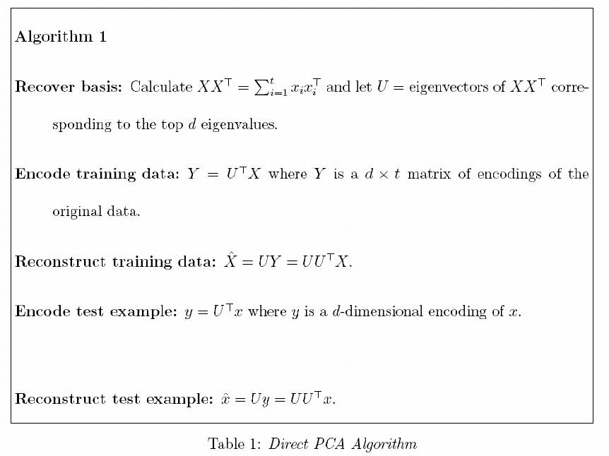
Other Notes:

   1. The mean of the data(X) must be 0.  This means we may have to preprocess the data by subtracting off the mean.
   2. Encoding the data means that we are projecting the data onto a lower dimensional subspace by taking the 
        inner product.  [math]\displaystyle{ U^T *X  }[/math] is a (d x n) matrix.
   3. When we reconstruct the training set, we are only using the top d dimensions.  This will eliminate the 
         dimensions that have lower variance (e.g. noise)
   4. We can compare the reconstructed test sample to the reconstructed training sample to classify the new data.