acceptance-Rejection Sampling
Acceptance-Rejection Sampling - May 14, 2009
Today, we continue the discussion on sampling (generating random numbers) from general distributions with the Acceptance/Rejection Method.
Acceptance/Rejection Method
Suppose we wish to sample from a target distribution [math]\displaystyle{ f(x) }[/math] that is difficult or impossible to sample from directly. Suppose also that we have a proposal distribution [math]\displaystyle{ g(x) }[/math] from which we have a reasonable method of sampling (e.g. the uniform distribution). Then, if there is a constant [math]\displaystyle{ c \ |\ c \cdot g(x) \geq f(x)\ \forall x }[/math], accepting samples drawn in successions from [math]\displaystyle{ c \cdot g(x) }[/math] with ratio [math]\displaystyle{ \frac {f(x)}{c \cdot g(x)} }[/math] close to 1 will yield a sample that follows the target distribution [math]\displaystyle{ f(x) }[/math]; on the other hand we would reject the samples if the ratio is not close to 1.
The following graph shows the pdf of [math]\displaystyle{ f(x) }[/math] (target distribution) and [math]\displaystyle{ c \cdot g(x) }[/math] (proposal distribution)
At x=7; sampling from [math]\displaystyle{ c \cdot g(x) }[/math] will yield a sample that follows the target distribution [math]\displaystyle{ f(x) }[/math]
At x=9; we will reject samples according to the ratio [math]\displaystyle{ \frac {f(x)}{c \cdot g(x)} }[/math] after sampling from [math]\displaystyle{ c \cdot g(x) }[/math]
Proof
Note the following:
- [math]\displaystyle{ Pr(X|accept) = \frac{Pr(accept|X) \times Pr(X)}{Pr(accept)} }[/math] (Bayes' theorem)
- [math]\displaystyle{ Pr(accept|X) = \frac{f(x)}{c \cdot g(x)} }[/math]
- [math]\displaystyle{ Pr(X) = g(x)\frac{}{} }[/math]
So, [math]\displaystyle{ Pr(accept) = \int^{}_x Pr(accept|X) \times Pr(X) dx }[/math] [math]\displaystyle{ = \int^{}_x \frac{f(x)}{c \cdot g(x)} g(x) dx }[/math] [math]\displaystyle{ = \frac{1}{c} \int^{}_x f(x) dx }[/math] [math]\displaystyle{ = \frac{1}{c} }[/math]
Therefore, [math]\displaystyle{ Pr(X|accept) = \frac{\frac{f(x)}{c\ \cdot g(x)} \times g(x)}{\frac{1}{c}} = f(x) }[/math] as required.
Procedure (Continuous Case)
- Choose [math]\displaystyle{ g(x) }[/math] (a density function that is simple to sample from)
- Find a constant c such that :[math]\displaystyle{ c \cdot g(x) \geq f(x) }[/math]
- Let [math]\displaystyle{ Y \sim~ g(y) }[/math]
- Let [math]\displaystyle{ U \sim~ Unif [0,1] }[/math]
- If [math]\displaystyle{ U \leq \frac{f(x)}{c \cdot g(x)} }[/math] then X=Y; else reject and go to step 1
Example:
Suppose we want to sample from Beta(2,1), for [math]\displaystyle{ 0 \leq x \leq 1 }[/math]. Recall:
- [math]\displaystyle{ Beta(2,1) = \frac{\Gamma (2+1)}{\Gamma (2) \Gamma(1)} \times x^1(1-x)^0 = \frac{2!}{1!0!} \times x = 2x }[/math]
- Choose [math]\displaystyle{ g(x) \sim~ Unif [0,1] }[/math]
- Find c: c = 2 (see notes below)
- Let [math]\displaystyle{ Y \sim~ Unif [0,1] }[/math]
- Let [math]\displaystyle{ U \sim~ Unif [0,1] }[/math]
- If [math]\displaystyle{ U \leq \frac{2Y}{2} = Y }[/math], then X=Y; else go to step 1
[math]\displaystyle{ c }[/math] was chosen to be 2 in this example since [math]\displaystyle{ \max \left(\frac{f(x)}{g(x)}\right) }[/math] in this example is 2. This condition is important since it helps us in finding a suitable [math]\displaystyle{ c }[/math] to apply the Acceptance/Rejection Method.
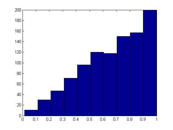
In MATLAB, the code that demonstrates the result of this example is:
   j = 1;
       while i < 1000
           y = rand;
           u = rand;
           if u <= y
               x(j) = y;
               j = j + 1;
               i = i + 1;
           end
       end
       hist(x);
The histogram produced here should follow the target distribution, [math]\displaystyle{ f(x) = 2x }[/math], for the interval [math]\displaystyle{ 0 \leq x \leq 1 }[/math].
The histogram shows the PDF of a Beta(2,1) distribution as expected.
The Discrete Case
The Acceptance/Rejection Method can be extended for discrete target distributions. The difference compared to the continuous case is that the proposal distribution [math]\displaystyle{ g(x) }[/math] must also be discrete distribution. For our purposes, we can consider g(x) to be a discrete uniform distribution on the set of values that X may take on in the target distribution.
Example
Suppose we want to sample from a distribution with the following probability mass function (pmf):
P(X=1) = 0.15
P(X=2) = 0.55
P(X=3) = 0.20
P(X=4) = 0.10
- Choose [math]\displaystyle{ g(x) }[/math] to be the discrete uniform distribution on the set [math]\displaystyle{ \{1,2,3,4\} }[/math]
- Find c: [math]\displaystyle{ c = \max \left(\frac{f(x)}{g(x)} \right)= 0.55/0.25 = 2.2 }[/math]
- Generate [math]\displaystyle{ Y \sim~ Unif \{1,2,3,4\} }[/math]
- Let [math]\displaystyle{ U \sim~ Unif [0,1] }[/math]
- If [math]\displaystyle{ U \leq \frac{f(x)}{2.2 \times 0.25} }[/math], then X=Y; else go to step 1
Limitations
If the proposed distribution is very different from the target distribution, we may have to reject a large number of points before a good sample size of the target distribution can be established. It may also be difficult to find such [math]\displaystyle{ g(x) }[/math] that satisfies all the conditions of the procedure.
We will now begin to discuss sampling from specific distributions.
Special Technique for sampling from Gamma Distribution
Recall that the cdf of the Gamma distribution is:
[math]\displaystyle{ F(x) = \int_0^{\lambda x} \frac{e^{-y}y^{t-1}}{(t-1)!} dy }[/math]
If we wish to sample from this distribution, it will be difficult for both the Inverse Method (difficulty in computing the inverse function) and the Acceptance/Rejection Method.
Additive Property of Gamma Distribution
Recall that if [math]\displaystyle{ X_1, \dots, X_t }[/math] are independent exponential distributions with mean [math]\displaystyle{ \lambda }[/math] (in other words, [math]\displaystyle{ X_i\sim~ Exp (\lambda) }[/math]), then [math]\displaystyle{ \Sigma_{i=1}^t X_i \sim~ Gamma (t, \lambda) }[/math]
It appears that if we want to sample from the Gamma distribution, we can consider sampling from t independent exponential distributions with mean [math]\displaystyle{ \lambda }[/math] (using the Inverse Method) and add them up. Details will be discussed in the next lecture.
