techniques for Normal and Gamma Sampling
Techniques for Normal and Gamma Sampling - May 19, 2009
We have examined two general techniques for sampling from distributions. However, for certain distributions more practical methods exist. We will now look at two cases,
Gamma distributions and Normal distributions, where such practical methods exist.
Gamma Distribution
Given the additive property of the gamma distribution,
If [math]\displaystyle{ X_1, \dots, X_t }[/math] are independent random variables with [math]\displaystyle{ X_i\sim~ Exp (\lambda) }[/math] then,
- [math]\displaystyle{ \Sigma_{i=1}^t X_i \sim~ Gamma (t, \lambda) }[/math]
We can use the Inverse Transform Method and sample from independent uniform distributions seen before to generate a sample following a Gamma distribution.
- Procedure
- Sample independently from a uniform distribution [math]\displaystyle{ t }[/math] times, giving [math]\displaystyle{ u_1,\dots,u_t }[/math]
- Sample independently from an exponential distribution [math]\displaystyle{ t }[/math] times, giving [math]\displaystyle{ x_1,\dots,x_t }[/math] such that,
[math]\displaystyle{ \begin{align} x_1 \sim~ Exp(\lambda)\\ \vdots \\ x_t \sim~ Exp(\lambda) \end{align} }[/math]
Using the Inverse Transform Method,
[math]\displaystyle{ \begin{align} x_i = -\frac {1}{\lambda}\log(u_i) \end{align} }[/math] - Using the additive property,
[math]\displaystyle{ \begin{align} X &{}= x_1 + x_2 + \dots + x_t \\ X &{}= -\frac {1}{\lambda}\log(u_1) - \frac {1}{\lambda}\log(u_2) \dots - \frac {1}{\lambda}\log(u_t) \\ X &{}= -\frac {1}{\lambda}\log(\prod_{i=1}^{t}u_i) \sim~ Gamma (t, \lambda) \end{align} }[/math]
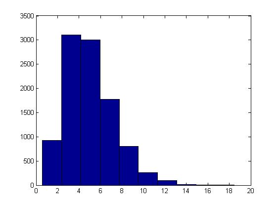
This procedure can be illustrated in Matlab using the code below with [math]\displaystyle{ t = 5, \lambda = 1 }[/math] :
U = rand(10000,5);
X = sum( -log(U), 2);
hist(X)
Normal Distribution
The cdf for the Standard Normal distribution is:
- [math]\displaystyle{ F(Z) = \int_{-\infty}^{Z}\frac{1}{\sqrt{2\pi}}e^{-x^2/2}dx }[/math]
We can see that the normal distribution is difficult to sample from using the general methods seen so far, eg. the inverse is not easy to obtain from F(Z); we may be able to use the Acceptance-Rejection method, but there are still better ways to sample from a Standard Normal Distribution.
=====Box-Muller Method===== [Add a picture WikiSysop 19:25, 1 June 2009 (UTC)]
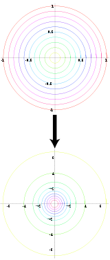 "Diagram of the Box Muller transform, which transforms uniformly distributed value pairs to normally distributed value pairs." [Box-Muller Transform, Wikipedia]
The Box-Muller or Polar method uses an approach where we have one space that is easy to sample in, and another with the desired distribution under a transformation. If we know such a transformation for the Standard Normal, then all we have to do is transform our easy sample and obtain a sample from the Standard Normal distribution.
- Properties of Polar and Cartesian Coordinates
- If x and y are points on the Cartesian plane, r is the length of the radius from a point in the polar plane to the pole, and θ is the angle formed with the polar axis then,
- [math]\displaystyle{ \begin{align} r^2 = x^2 + y^2 \end{align} }[/math]
- [math]\displaystyle{ \tan(\theta) = \frac{y}{x} }[/math]
- [math]\displaystyle{ \begin{align} x = r \cos(\theta) \end{align} }[/math]
- [math]\displaystyle{ \begin{align} y = r \sin(\theta) \end{align} }[/math]
Let X and Y be independent random variables with a standard normal distribution,
- [math]\displaystyle{ X \sim~ N(0,1) }[/math]
- [math]\displaystyle{ Y \sim~ N(0,1) }[/math]
also, let [math]\displaystyle{ r }[/math] and [math]\displaystyle{ \theta }[/math] be the polar coordinates of (x,y). Then the joint distribution of independent x and y is given by,
- [math]\displaystyle{ \begin{align} f(x,y) = f(x)f(y) &{}= \frac{1}{\sqrt{2\pi}}e^{-\frac{x^2}{2}}\frac{1}{\sqrt{2\pi}}e^{-\frac{y^2}{2}} \\ &{}=\frac{1}{2\pi}e^{-\frac{x^2+y^2}{2}} \end{align} }[/math]
It can also be shown that the joint distribution of r and θ is given by,
- [math]\displaystyle{ \begin{matrix} f(r,\theta) = \frac{1}{2}e^{-\frac{d}{2}}*\frac{1}{2\pi},\quad d = r^2 \end{matrix} }[/math]
Note that [math]\displaystyle{ \begin{matrix}f(r,\theta)\end{matrix} }[/math] consists of two density functions, Exponential and Uniform, so assuming that r and [math]\displaystyle{ \theta }[/math] are independent [math]\displaystyle{ \begin{matrix} \Rightarrow d \sim~ Exp(1/2), \theta \sim~ Unif[0,2\pi] \end{matrix} }[/math]
- Procedure for using Box-Muller Method
- Sample independently from a uniform distribution twice, giving [math]\displaystyle{ \begin{align} u_1,u_2 \sim~ \mathrm{Unif}(0, 1) \end{align} }[/math]
- Generate polar coordinates using the exponential distribution of d and uniform distribution of θ,
[math]\displaystyle{ \begin{align} d = -2\log(u_1),& \quad r = \sqrt{d} \\ & \quad \theta = 2\pi u_2 \end{align} }[/math] - Transform r and θ back to x and y,
[math]\displaystyle{ \begin{align} x = r\cos(\theta) \\ y = r\sin(\theta) \end{align} }[/math]
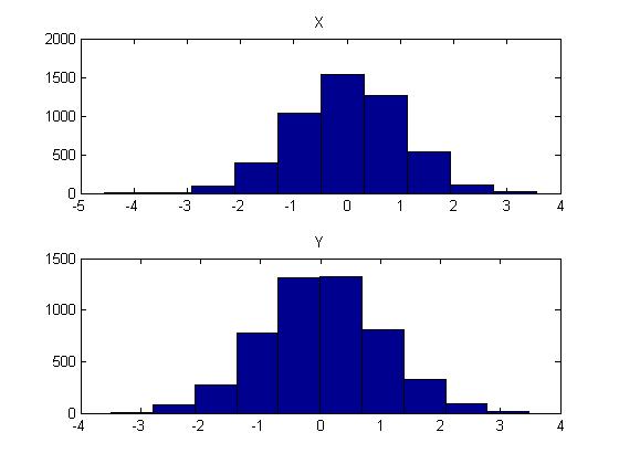
Notice that the Box-Muller Method generates a pair of independent Standard Normal distributions, x and y.
This procedure can be illustrated in Matlab using the code below:
u1 = rand(5000,1);
u2 = rand(5000,1);

d = -2*log(u1);
theta = 2*pi*u2;

x = d.^(1/2).*cos(theta);
y = d.^(1/2).*sin(theta);

figure(1);

subplot(2,1,1);
hist(x);
title('X');
subplot(2,1,2);
hist(y);
title('Y');
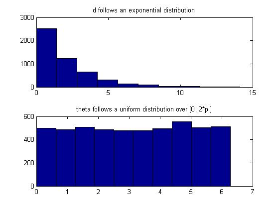
Also, we can confirm that d and theta are indeed exponential and uniform random variables, respectively, in Matlab by:
subplot(2,1,1);
hist(d);
title('d follows an exponential distribution');
subplot(2,1,2);
hist(theta);
title('theta follows a uniform distribution over [0, 2*pi]');
Useful Properties (Single and Multivariate)
Box-Muller can be used to sample a standard normal distribution. However, there are many properties of Normal distributions that allow us to use the samples from Box-Muller method to sample any Normal distribution in general.
- Properties of Normal distributions
- [math]\displaystyle{ \begin{align} \text{If } & X = \mu + \sigma Z, & Z \sim~ N(0,1) \\ &\text{then } X \sim~ N(\mu,\sigma ^2) \end{align} }[/math]
- [math]\displaystyle{ \begin{align} \text{If } & \vec{Z} = (Z_1,\dots,Z_d)^T, & Z_1,\dots,Z_d \sim~ N(0,1) \\ &\text{then } \vec{Z} \sim~ N(\vec{0},I) \end{align} }[/math]
- [math]\displaystyle{ \begin{align} \text{If } & \vec{X} = \vec{\mu} + \Sigma^{1/2} \vec{Z}, & \vec{Z} \sim~ N(\vec{0},I) \\ &\text{then } \vec{X} \sim~ N(\vec{\mu},\Sigma) \end{align} }[/math]
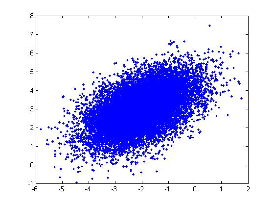
These properties can be illustrated through the following example in Matlab using the code below:
Example: For a Multivariate Normal distribution [math]\displaystyle{ u=\begin{bmatrix} -2 \\ 3 \end{bmatrix} }[/math] and [math]\displaystyle{ \Sigma=\begin{bmatrix} 1&0.5\\ 0.5&1\end{bmatrix} }[/math]
u = [-2; 3];
sigma = [ 1 1/2; 1/2 1];

r = randn(15000,2);
ss = chol(sigma);

X = ones(15000,1)*u' + r*ss;
plot(X(:,1),X(:,2), '.');
Note: In the example above, we had to generate the square root of [math]\displaystyle{ \Sigma }[/math] using the Cholesky decomposition,
ss = chol(sigma);
which gives [math]\displaystyle{ ss=\begin{bmatrix} 1&0.5\\ 0&0.8660\end{bmatrix} }[/math]. Matlab also has the sqrtm function:
ss = sqrtm(sigma);
which gives a different matrix, [math]\displaystyle{ ss=\begin{bmatrix} 0.9659&0.2588\\ 0.2588&0.9659\end{bmatrix} }[/math], but the plot looks about the same (X has the same distribution).
