visualizing Data using t-SNE
Introduction
The paper <ref>Laurens van der Maaten, and Geoffrey Hinton. Visualizing Data using t-SNE. Journal of Machine Learning Research, 9: 2579-2605, 2008</ref> introduced a new nonlinear dimensionally reduction technique that "embeds" high-dimensional data into low-dimensional space. This technique is a variation of the Stochastic Neighbor embedding (SNE) that was proposed by Hinton and Roweis in 2002 <ref>G.E. Hinton and S.T. Roweis. Stochastic Neighbor embedding. In Advances in Neural Information Processing Systems, vol. 15, pp, 883-840, Cambridge, MA, USA, 2002. The MIT Press.</ref>, where the high-dimensional Euclidean distances between datapoints are converted into the conditional probability to describe their similarities. t-SNE, based on the same idea, is aimed to be easier for optimization and to solve the "crowding problem". In addition, the author showed that t-SNE can be applied to large data sets as well, by using random walks on neighborhood graphs. The performance of t-SNE is demonstrated on a wide variety of data sets and compared with many other visualization techniques.
Stochastic Neighbor Embedding
In SNE, the high-dimensional Euclidean distances between datapoints is first converted into probabilities. The similarity of datapoint [math]\displaystyle{ \mathbf x_j }[/math] to datapoint [math]\displaystyle{ \mathbf x_i }[/math] is then presented by the conditional probability, [math]\displaystyle{ \mathbf p_{j|i} }[/math], that [math]\displaystyle{ \mathbf x_i }[/math] would pick [math]\displaystyle{ \mathbf x_j }[/math] as its neighbor when neighbors are picked in proportion to their probability density under a Gaussian centered on [math]\displaystyle{ \mathbf x_i }[/math]. The [math]\displaystyle{ \mathbf p_{j|i} }[/math] is given as
where [math]\displaystyle{ \mathbf k }[/math] is the effective number of the local neighbors, [math]\displaystyle{ \mathbf \sigma_i }[/math] is the variance of the Gaussian that is centered on [math]\displaystyle{ \mathbf x_i }[/math], and for every [math]\displaystyle{ \mathbf x_i }[/math], we set [math]\displaystyle{ \mathbf p_{i|i} = 0 }[/math]. It can be seen from this definition that, the closer the datapoints are, the higher the [math]\displaystyle{ \mathbf p_{j|i} }[/math] is. For the widely separated datapoints, [math]\displaystyle{ \mathbf p_{j|i} }[/math] is almost infinitesimal.
With the same idea, in the low-dimensional space, we model the similarity of map point [math]\displaystyle{ \mathbf y_j }[/math] to [math]\displaystyle{ \mathbf y_i }[/math] by the conditional probability [math]\displaystyle{ \mathbf q_{j|i} }[/math], which is given by
where we set the variance of the Gaussian [math]\displaystyle{ \mathbf \sigma_i }[/math] to be [math]\displaystyle{ \frac{1}{\sqrt{2} } }[/math] (a different value will only result in rescaling of the final map). And again, we set [math]\displaystyle{ \mathbf q_{i|i} = 0 }[/math].
If the low-dimensional map points correctly present the high-dimensional datapoints, their conditional probabilities [math]\displaystyle{ \mathbf q_{j|i} }[/math] and [math]\displaystyle{ \mathbf p_{j|i} }[/math] should be equal. Therefore, the aim of SNE is to minimize the mismatch between [math]\displaystyle{ \mathbf q_{j|i} }[/math] and [math]\displaystyle{ \mathbf p_{j|i} }[/math]. This is achieved by minimizing the sum of Kullback-leibler divergence (a non-symmetric measure of the difference between two probability distributions) over all datapoints. The cost function of SNE is then expressed as
where [math]\displaystyle{ \mathbf P_i }[/math] and [math]\displaystyle{ \mathbf Q_i }[/math] are the conditional probability distribution over all other points for given [math]\displaystyle{ \mathbf x_i }[/math] and [math]\displaystyle{ \mathbf y_i }[/math]. Since the Kullback-leibler divergence is asymmetric, there is a large cost for using a small [math]\displaystyle{ \mathbf q_{j|i} }[/math] to model a big [math]\displaystyle{ \mathbf p_{j|i} }[/math], while a small cost for using a large [math]\displaystyle{ \mathbf q_{j|i} }[/math] to model a small [math]\displaystyle{ \mathbf p_{j|i} }[/math]. Therefore, the SNE cost function focuses more on local structure. It enforces both keeping the images of nearby objects nearby and keeping the images of widely separated objects relatively far apart.
The remaining parameter [math]\displaystyle{ \mathbf \sigma_i }[/math] here is selected by performing a binary search for the value of [math]\displaystyle{ \mathbf \sigma_i }[/math] that produces a [math]\displaystyle{ \mathbf P_i }[/math] with a fixed perplexity (a measure of the effective number of neighbors, which is related to [math]\displaystyle{ \mathbf k }[/math], defined as the two to the power of Shannon entropy of [math]\displaystyle{ P_i }[/math]) that is selected by the user.
To minimize the cost function, gradient descent method is used. The gradient then is given as
which is simple and has a nice physical interpretation. The gradient can be seen as the resultant force induced by a set of springs between the map point [math]\displaystyle{ \mathbf y_i }[/math] and all other neighbor points [math]\displaystyle{ \mathbf y_j }[/math], where the force is exerted in the direction [math]\displaystyle{ \mathbf (y_i-y_j) }[/math] and the stiffness of the spring is [math]\displaystyle{ \mathbf ([p_{j|i}-q_{j|i}]+[p_{i|j}-q_{i|j}]) }[/math].
t-Distributed Stochastic Neighbor Embedding
Although SNE showed relatively good visualizations, it has two main problems: difficulty in optimization and the "crowding problem". t-Distributed Stochastic Neighbor Embedding (t-SNE), which is a variation of SNE, is aimed to alleviate these problems. The cost function of t-SNE differs from the one of SNE in two ways: (1) it uses a symmetric version of the SNE cost function, and (2) it uses a Student-t distribution instead of Gaussian to compute the conditional probability in the low-dimensional space.
Symmetric SNE
In symmetric SNE, instead of the sum of the Kullback-Leibler divergences between the conditional probabilities, the cost function is a single Kullback-Leibler divergence between two joint probability distributions, [math]\displaystyle{ \mathbf P }[/math] in the high-dimensional space and [math]\displaystyle{ \mathbf Q }[/math] in the low-dimensional space.
In this case, the pairwise similarities of the data points in high-dimensional space is given by,
and [math]\displaystyle{ \mathbf q_{ij} }[/math] in low-dimensional space is
where [math]\displaystyle{ \mathbf p_{ii} }[/math] and [math]\displaystyle{ \mathbf q_{ii} }[/math] are still zero. When a high-dimensional datapoint [math]\displaystyle{ \mathbf x_i }[/math] is a outlier (far from all the other points), we set [math]\displaystyle{ \mathbf{p_{ij}=\frac {(p_{j|i}+p_{i|j})}{2n}} }[/math] to ensure that [math]\displaystyle{ \sum_{j} p_{ij} \gt \frac {1}{2n} }[/math] for all [math]\displaystyle{ \mathbf x_i }[/math]. This will make sure that all [math]\displaystyle{ \mathbf x_i }[/math] make significant contribution to the cost function, which is given as
As we can see, by definition, we have [math]\displaystyle{ \mathbf p_{ij} = p_{ji} }[/math] and [math]\displaystyle{ \mathbf q_{ij} = q_{ji} }[/math]. This is why it is called symmetric SNE.
From the cost function, we have the gradient as simple as
which is the main advantage of symmetric SNE.
The Crowding Problem
The "crowding problem" that are addressed in the paper is defined as: "the area of the two-dimensional map that is available to accommodate moderately distant datapoints will not be nearly large enough compared with the area available to accommodate nearby datepoints". This happens when the datapoints are distributed in a region on a high-dimensional manifold around [math]\displaystyle{ i }[/math], and we try to model the pairwise distances from [math]\displaystyle{ i }[/math] to the datapoints in a two-dimensional map. For example, it is possible to have 11 datapoints that are mutually equidistant in a ten-dimensional manifold but it is not possible to model this faithfully in a two-dimensional map. Therefore, if the small distances can be modeled accurately in a map, most of the moderately distant datapoints will be too far away in the two-dimensional map. In SNE, this will result in very small attractive force from datapoint [math]\displaystyle{ i }[/math] to these too-distant map points. The very large number of such forces collapses together the points in the center of the map and prevents gaps from forming between the natural clusters. This phenomena, crowding problem, is not specific to SNE and can be observed in other local techniques such as Sammon mapping as well.
According to Cook et al.(2007), adding a slight repulsion can address this problem. Using a uniform backgorund model with a small mixing proportion, [math]\displaystyle{ \,\rho }[/math], helps [math]\displaystyle{ \,q_{ij} }[/math] never fall below [math]\displaystyle{ \frac{2\rho}{n(n-1)} }[/math]. In this technique, called UNI-SNE, [math]\displaystyle{ \,q_{ij} }[/math] will be larger than [math]\displaystyle{ \,p_{ij} }[/math] even for the far-apart datapoints.
Compensation for Mismatched Dimensionality by Mismatched Tails
Since the crowding problem is caused by the unwanted attractive forces between map points that present moderately dissimilar datapoints nearby, one solution is to model these datapoints by a much larger distance in the map to eliminates the attractive forces. This can be achieved by using a probability distribution that has much heavier tails than a Gaussian to convert the distances into probabilities in the low-dimensional space. Student t-distribution is selected because it is closely related to the Gaussian distribution, but it is much faster computationally since it does not involve any exponential. In addition, t-distribution as a heavier tail distribution allows a temperate distance to be modeled by a larger distance in the map that eliminates the unwanted attractive forces between dissimilar data points.
In t-SNE, Student t-distribution with one degree of freedom is employed in the low-dimensional map. Based on the symmetric SNE, the joint probabilities in high-dimensional [math]\displaystyle{ \mathbf p_{ij} }[/math] are still
while the joint probabilities [math]\displaystyle{ \mathbf q_{ij} }[/math] are defined as
The gradient of the Kullback-Leibler divergence between [math]\displaystyle{ P }[/math] and the Student-t based joint probability distribution [math]\displaystyle{ Q }[/math] is then given by
Compared with the gradients of SNE and UNI-SNE <ref> J.A. Cook, and I. Sutskever et al.. Visualizing similarity data with a mixture of maps. In Proceeding of the 11th International Conference on Artificial Intelligence and Statistics, volume 2, page, 67-74, 2007.</ref>, the t-SNE gradients introduces strong repulsions between the dissimilar datapoints that are modeled by small pairwise distance in the low-dimensional map. This well prevents the crowding problem that was mentioned above. At the same time, these repulsions do not go to infinity, which prevents the dissimilar datapoints from being too far apart. Therefore, the t-SNE models dissimilar datepoints by means of large pairwise distance, while models similar datapoints by means of small pairwise distance. This results in the good representation of both local and global structure of the high-dimensional data.
Optimization Methods for t-SNE
One ways to optimize the t-SNE cost function is to use a momentum term to reduce the number of required iteration. To further improve the modeling results, two tricks called "early compression" and "early exaggeration" can be used. The "early compression" is to force the map points to stay close together at the early stage of the optimization so that it is easy for explore the space of possible global organizations of the data. "Early exaggeration" is to multiply all the [math]\displaystyle{ \mathbf p_{ij} }[/math]'s by a [math]\displaystyle{ n\gt 1 }[/math] in the initial stages of the optimization. This will make all the [math]\displaystyle{ \mathbf q_{ij} }[/math]'s too small to model their corresponding [math]\displaystyle{ \mathbf p_{ij} }[/math]'s, so that the modeling are forced to focus on large [math]\displaystyle{ \mathbf p_{ij} }[/math]'s. This leads to the formation of tight widely separated clusters in the map, which makes it very easy to move around the clusters for a good global organization.
Experiments with Different Data Sets
The author performed t-SNE on five data sets and compared the results with seven other non-parametric dimensional reduction techniques to evaluate t-SNE. The five data sets that were employed are: (1) the MNIST data set, (2) the Olivetti faces data set, (3) the COIL-20 data set, (4) the word-feature data set, and (5) the Netflix data set.
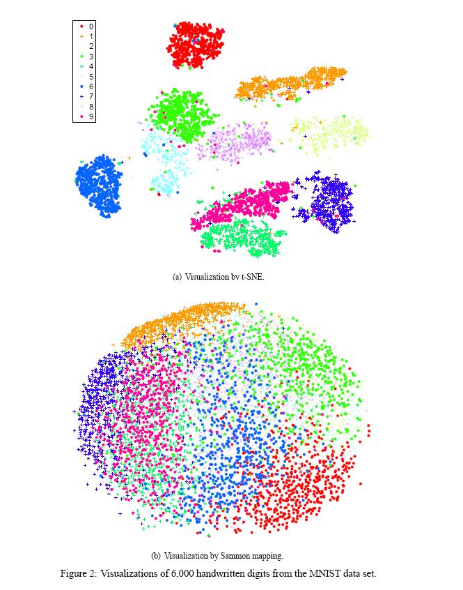
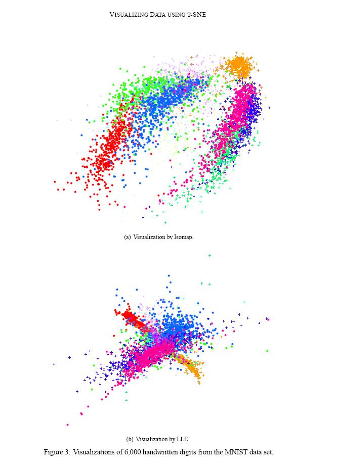
When performed t-SNE on the MNIST data set, t-SNE constructed a map with clear and clean separations between different digit classes. At the same time, most of the local structures of the data is captured as well. On the another hand, Isomap and LLE provide very little insight into the class structure of the data, while Sammon map models the classes fairly well but does not separate them clearly.
We show the results of our experiments with t-SNE, Sammon mapping, Isomap, and LLE on the MNIST data set in figures 2 and 3.
The results is a good indicator of strong performance of t-SNE compared to the other techniques. In particular, Sammon mapping constructs a “ball” in which only three classes (representing the digits 0, 1, and 7) are somewhat separated from the other classes. Isomap and LLE produce solutions in which there are large overlaps between the digit classes. In contrast, t-SNE constructs a map in which the separation between the digit classes is almost perfect. Moreover, detailed inspection of the t-SNE map reveals that much of the local structure of the data (such as the orientation of the ones) is captured as well. The map produced by t-SNE contains some points that are clustered with the wrong class, but most of these points correspond to distorted digits many of which are difficult to identify.


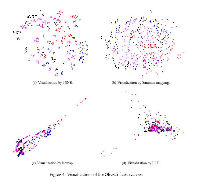
In figure 4 we have showed the results of applying t-SNE, Sammon mapping, Isomap, and LLE to the Olivetti faces data set. Similar to what we had before, Isomap and LLE produce solutions that provide little insight into the class structure of the data. Since Sammon mapping models many of the members of each class fairly close together, but none of the classes are clearly separated in the Sammon map, it produces a much better map compared to the other methods. In contrast, t-SNE does a much better job of revealing the natural classes in the data. Some individuals have their ten images split into two clusters, usually because a subset of the images have the head facing in a significantly different direction, or because they have a very different expression or glasses. For these individuals, it is not clear that their ten images form a natural class when using Euclidean distance in pixel space.

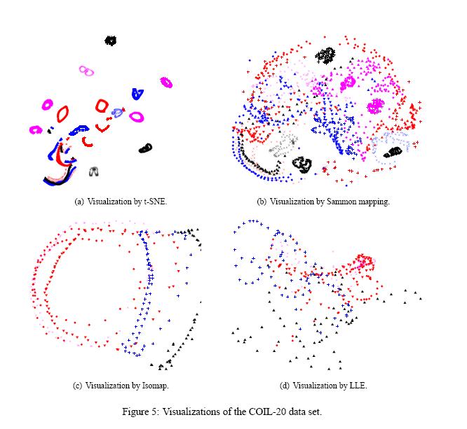
Figure 5 shows the results of applying t-SNE, Sammon mapping, Isomap, and LLE to the COIL-20 data set. An interesting observation in this ection is that for many of the 20 objects, t-SNE accurately represents the one-dimensional manifold of viewpoints as a closed loop. For objects which look similar from the front and the back, t-SNE distorts the loop so that the images of front and back are mapped to nearby points. For the four types of toy car in the COIL-20 data set (the four aligned “sausages” in the bottom-left of the t-SNE map), the four rotation manifolds are aligned by the orientation of the cars to capture the high similarity between different cars at the same orientation. This prevents t-SNE from keeping the four manifolds clearly separate.
An interesting point shown in figure 5 is that the other three techniques are not nearly as good at cleanly separating the manifolds that correspond to very different objects. On top of that Isomap and LLE only visualize a small number of classes from the COIL-20 data set, because the data set comprises a large number of widely separated sub-manifolds that give rise to small connected components in the neighborhood graph.

t-SNE for Large Data Sets
Due to its computational and memory complexity, it is infeasible to apply the standard version of t-SNE to large data sets (which contain more than 10,000 data points). To solve this problem, t-SNE is modified to display a random set of landmark points in the way that uses the information of the whole data set. First, a neighborhood graph for all the data points is created under a selected number of neighbors. Then, for each of the selected landmark point, a random walk is defined, which starts from that landmark point and terminates as soon as it lands on another landmark point. [math]\displaystyle{ \mathbf p_{j|i} }[/math] denotes the fraction of random walk starting at landmark point [math]\displaystyle{ x_i }[/math] and terminate at landmark point [math]\displaystyle{ x_j }[/math]. To avoid the "short-circuits" caused by a noisy datapoint, the random walk-based affinity measure integrates over all paths through the neighborhood graph. The random walk-based similarities [math]\displaystyle{ \mathbf p_{j|i} }[/math] can be computed by explicitly performing the random walks on the neighborhood graph, or using an analytical solution <ref> L. Grady, 2006, Random walks for image segmentation. IEEE Transactions on Pattern Analysis and Machine Intelligence, 28(11): 1768-1783, 2006. </ref>, which is more appropriate for very large data sets. In fact, the important factor is the probability of a random walk which has been initiated from a landmark point, and is going to be terminated at another landmark point. Kakutani (in 1945) has shown that to compute the probability that a random walk initiated from a non-landmark point first reaches a specific landmark point, one can solve the combinatorial Dirichlet problem in which the boundary conditions are at the locations of the landmark points, the considered landmark point is fixed to unity, and the other landmarks points are set to zero.
Weaknesses of t-SNE
Although t-SNE has demonstrated to be a favorable technique for data visualization, there are three potential weaknesses with this technique. (1) The paper only focuses on the date visualization using t-SNE, that is, embedding high-dimensional date into a two- or three-dimensional space. However, this behavior of t-SNE presented in the paper cannot readily be extrapolated to d>3 dimensions due to the heavy tails of the Student t-distribution. (2) t-SNE might be less successful when applied to data sets with a high intrinsic dimensionality. This is a result of the local linearity assumption on the manifold that t-SNE makes by employing Euclidean distance to present the similarity between the datapoints. (3) Another major weakness of t-SNE is that the cost function is not convex. This leads to the problem that several optimization parameters need to be chosen and the constructed solutions depending on these parameters may be different each time t-SNE is run from an initial random configuration of the map points.
References
<references/>