nonlinear Dimensionality Reduction by Semidefinite Programming and Kernel Matrix Factorization
Introduction
In recent work, Semidefinite programming (SDE) that learns a kernel matrix by maximizing variance while preserving the distance and angles between nearest neigbors has been introduced. Although it has many advantages such as optimization convexity, it sufferes from computational cost for large problems. In this paper <ref>K. Q. Weinberger et al. Graph Laplacian Regularization for Larg-Scale Semidefinite Programming, Proceedings of the the Tenth international workshop on Artificial Intelligence and Statistics (AISTATS-05), pages 381-388, Barbados, West Indies, 2005.</ref> , a new framework based on factorization of the entire kernel matrix in terms of a much smaller submatrix of inner products between randomly chosen landmarks has been proposed.
Semidefinite Embedding
Given high dimensional vectors [math]\displaystyle{ \,\{x_1, x_2, ..., x_n\} \in R^D }[/math] lying on or near a manifold that can be embeded in [math]\displaystyle{ \,d\ll D }[/math] dimensions to produce low dimensional vectors [math]\displaystyle{ \,\{y_1, y_2, ..., y_n\} \in R^d }[/math], the goal is to find d and produce an appropriate embedding. The algorithm starts with computing k-nearest neighbors of each input and adding a constraint to preserve distances and angles between k-nearest neighbors:
[math]\displaystyle{ \,\|y_i-y_j\|^2 = \|x_i-x_j\|^2 }[/math] for all (i,j) in k-nearest neighbors (2)
and also a constraint on outputs to be centerd on the origin:
[math]\displaystyle{ \,\sum_i{y_i} = 0 }[/math] (3)
And maximizining the variance of outputs will be the final step:
[math]\displaystyle{ \,var(y)=\sum_i{\|y_i\|^2} }[/math] (4)
(since (3), it is cleat that [math]\displaystyle{ \sum_{i,j}{\|y_i - y_j\|^2} = 2\sum_i{\|y_i\|^2} }[/math], therefore maximizing the variance of Y will stretch the distances and force the data to lie on a lower dimensional subspace)
Assuming [math]\displaystyle{ \,K_{ij}=y_i^T . y_j }[/math], the above optimzation problem can be reformulated as an SDE:
Maximize trace(K) subject to :
1) [math]\displaystyle{ \,K\succeq 0 }[/math]
2)[math]\displaystyle{ \,\sum_{ij}K_{ij}=0 }[/math]
3) For all (i,j) such that [math]\displaystyle{ \,\eta_{ij}=1 }[/math],
[math]\displaystyle{ \,K_{ii}-2K_{ij}+K_{jj}=\|x_i-x_j\|^2 }[/math]
the top d eigenvalues and eigenvectors of the kernel matrix will be used to derive the embedding. Here, learning the kernel matrix dominates the total computation time.
Kernel Matrix Factorization
As we saw in the last section, learning the kernel matrix takes a lot of computational time. Therefore, if we can approximate it by a much smaller matrix , the computation time will be drastically improved. This can be done through the following steps:
First, reconstructing high dimensional datasate [math]\displaystyle{ \,\{x_i\}_{i=1}^n }[/math] from m randomly chosen landmarks [math]\displaystyle{ \,\{\mu_{\alpha}\}_{\alpha=1}^m }[/math] :
[math]\displaystyle{ \,\hat{x_i} = \sum_{\alpha}{Q_{i\alpha}\mu_{\alpha}} }[/math]
Based on the similar intuition from locally linear embedding (LLE), the same linear transformation (Q) can be used to reconstruct the output:
[math]\displaystyle{ \,\hat{y_i} = \sum_{\alpha}{Q_{i\alpha}l_{\alpha}} }[/math] (6)
Now, if we make the approximation:
[math]\displaystyle{ \,K_{ij}=y_i.y_j \approx \hat{y_i}.\hat{y_j} }[/math] (7)
substituting (6) into (7) gives [math]\displaystyle{ \,K\approx QLQ^T }[/math] where [math]\displaystyle{ \,L_{\alpha\beta} = l_{\alpha}.l_{\beta} }[/math]
Reconstructing from landmarks
To derive Q, we assume that the manifold can be locally approximated by a linear subspace. Therefore, each input in the high dimensional space can be reconstructed by a weighted sum of its r-nearest neighbors. These weights are found by :
Minimize :[math]\displaystyle{ \,\varepsilon(W)=\sum_i{\|x_i-\Sigma_j{W_{ij}x_j}\|^2} }[/math]
subject to:[math]\displaystyle{ \,\Sigma_j{W_{ij}}=1 }[/math] for all j
and [math]\displaystyle{ \,W_{ij}=0 }[/math] if [math]\displaystyle{ \,x_i }[/math] are not r-nearest neighbor of [math]\displaystyle{ \,x_j }[/math]
Rewriting the reconstruction error as function of inputs will give us:
[math]\displaystyle{ \,\varepsilon(X)=\sum_{ij}{\phi_{ij}x_i.x_j} }[/math]
where [math]\displaystyle{ \,\phi = (I_n-W)^T(I_n-W) }[/math] or
[math]\displaystyle{ \,\phi=\begin{bmatrix} \overbrace{\phi^{ll}}^{m} & \overbrace{\phi^{lu}}^{n-m} \\ \phi^{ul} & \phi^{uu}\end{bmatrix} }[/math]
and the solution will be:
[math]\displaystyle{ \,Q=\begin{bmatrix} I_m \\ -(\phi^{uu})^{-1}\phi^{ul}\end{bmatrix} }[/math]
As [math]\displaystyle{ \,W_{ij} }[/math] are invariant to translations and rotations of each input and its r-nearsest neighbors, the same weights can be used to reconstruct [math]\displaystyle{ \,y_i }[/math]
Embedding the landmarks
Considering the factorization [math]\displaystyle{ \,K\approx QLQ^T }[/math], we will get the following SDP:
Maximize trace([math]\displaystyle{ \,QLQ^T }[/math]) subject to :
1) [math]\displaystyle{ \,L\succeq 0 }[/math]
2)[math]\displaystyle{ \,\sum_{ij}(QLQ^T)_{ij}=0 }[/math]
3) For all (i,j) such that [math]\displaystyle{ \,\eta_{ij}=1 }[/math],
[math]\displaystyle{ \,(QLQ^T)_{ii}-2(QLQ^T)_{ij}+(QLQ^T)_{jj}\leq\|x_i-x_j\|^2 }[/math]
Because the matrix factorization is an approximate, the distance constraint has changed from equality to inequality.
The computation time in semidefinite programming depends on the matrix size and the number of constraints. Here, the matrix size in lSDE is much smaller than SDE. The number of constraints are the same. However, the constraints in lSDE are not sparse and this may lead to an lSDE even slower than SDE. To overcome this problem, one can feed an initial subset of constraints like just centering and semidifiniteness instead of the whole constraints. In the case that the solution violates the unused constraints, these will be added to the problem and the SDP solver will be run again.
Experimental Results
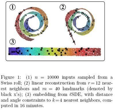
In the first experiment, Figure 1<ref>
The same paper. Figure 1
</ref>, only 1205 out of 43182 constraints had to be enforced based on Table 2.
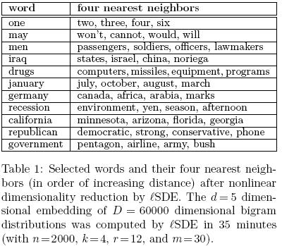
In the second experiment, Table 1<ref>
The same paper. Table 1
</ref>, despite the huge dimensionality reduction from D=60000 to d=5, many expected neighbors were preserved.
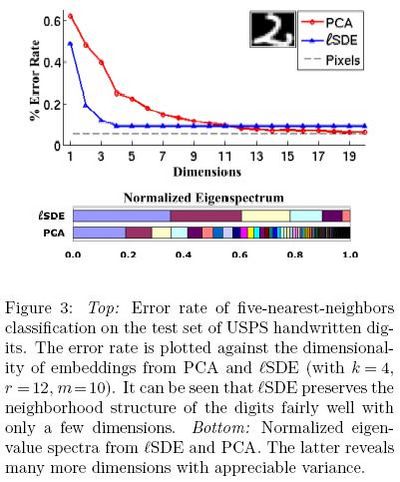
In the third experiment, Figure 2<ref>
The same paper. Figure 2
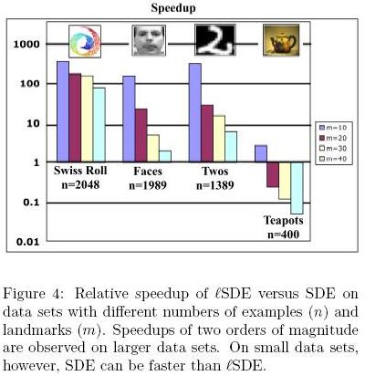
</ref>, the results from [math]\displaystyle{ lSDE }[/math] are differnet from the results from SDE, but they get close to each other with increasing number of landmarks. Here, as shown in Figure 4<ref>
The same paper. Figure 4
</ref>, [math]\displaystyle{ lSDE }[/math] is slower than SDE. Because the ddataset is too small and has a particular cyclic structure so that incremental scheme for adding constraints doesn't work well.

References
<references/>