continuous space language models
Introduction
This paper describes the use of a neural network language model for large vocabulary continuous speech recognition. The underlying idea of this approach is to attack the data sparseness problem by performing the language model probability estimation in a continuous space. Highly efficient learning algorithms are described that enable the use of training corpora of several hundred million words. It is also shown that this approach can be incorporated into a large vocabulary continuous speech recognizer using a lattice re scoring framework at a very low additional processing time
In certain fields of study such as speech recognition or machine translation, for some acoustic signal [math]\displaystyle{ \,x }[/math] or the source sentence to be translated [math]\displaystyle{ \,e }[/math], it is common to model these problems as finding the sequence of words [math]\displaystyle{ \,w^* }[/math] that has the highest probability of occurring given [math]\displaystyle{ \,x }[/math] or [math]\displaystyle{ \,e }[/math]. This can be written as:
[math]\displaystyle{ w^* = arg\ \underset {w}{max} P(w|x) = arg\ \underset{w}{max} P(x|w)P(w) }[/math]
An acoustic or translation model can then be used for [math]\displaystyle{ \,P(x|w) }[/math], similar to the idea behind LDA and QDA, and it remains to create a language model [math]\displaystyle{ \,P(w) }[/math] to estimate the probability of any sequence of words [math]\displaystyle{ \,w }[/math].
This is commonly done through the back-off n-grams model and the purpose behind this research paper is to use a neural network to better estimate [math]\displaystyle{ \,P(w) }[/math].
Back-off n-grams Model
A sequence of words will be defined as [math]\displaystyle{ \,w^i_1=(w_1,w_2,\dots,w_i) }[/math] and the formula for the probability [math]\displaystyle{ \,P(w) }[/math] can be rewritten as:
[math]\displaystyle{ P(w^n_1)=P(w_1,w_2,\dots,w_n)=P(w_1)\prod_{i=2}^n P(w_i|w^{i-1}_1) }[/math]
It is common to estimate [math]\displaystyle{ \,P(w_i|w^{i-1}_1) }[/math] through:
[math]\displaystyle{ \,P(w_i|w^{i-1}_1)\approx\frac{\mbox{number of occurrence of the sequence} (w_1,\dots,w_i)}{\mbox{number of occurrence of the sequence} (w_1,\dots,w_{i-1})} }[/math]
However, it is practically impossible to have a training set large enough to contain every possible sequence of words if the sequence is long enough and some sequences would have an incorrect probability of 0 simply because it is not in the training set. This is known as the data sparseness problem. This problem is commonly resolved by considering only the last n-1 words instead of the whole context. However, even for small n, certain sequences could still be missing.
To solve this issue, a technique called back-off n-grams is used and the general formula goes as follows:
[math]\displaystyle{ \,P(w_i|w^{i-1}_1) = \begin{cases} \frac{\mbox{number of occurrence of the sequence}\ (w_1,\dots,w_i)}{\mbox{number of occurrence of the sequence}\ (w_1,\dots,w_{i-1})}, & \mbox{if number of occurrence of}\ (w_1,\dots,w_i)\ \mbox{is greater than some constant K} \\ \alpha P(w_i|w^{i-1}_2), & \mbox{otherwise} \end{cases} }[/math]
[math]\displaystyle{ \,\alpha }[/math] is typically a discounting factor that is less than 1 to account for the lack of direct data. It usually depends on the word sequence.
The general algorithm is then, if the data set does contain the sequence then calculate probability directly. Otherwise, apply a discounting factor and calculate the conditional probability with the first word in the sequence removed. For example, if the word sequence was "The dog barked" and it did not exist in the training set then the formula would be written as:
[math]\displaystyle{ \,P(\mbox{barked}|\mbox{the,dog}) \approx \alpha P(\mbox{barked}|\mbox{dog}) }[/math]
Model
The neural network language model has to perform two tasks: first, project all words of the context [math]\displaystyle{ \,h_j }[/math] = [math]\displaystyle{ \,w_{j-n+1}^{j-1} }[/math] onto a continuous space, and second, calculate the language model probability [math]\displaystyle{ P(w_{j}=i|h_{j}) }[/math]. The researchers for this paper sought to find a better model for this probability than the back-off n-grams model. Their approach was to map the n-1 words sequence onto a multi-dimension continuous space using a layer of neural network followed by another layer to estimate the probabilities of all possible next words. The formulas and model goes as follows:
For some sequence of n-1 words, encode each word using 1 of K encoding, i.e. 1 where the word is indexed and zero everywhere else. Label each 1 of K encoding by [math]\displaystyle{ (w_{j-n+1},\dots,w_j) }[/math] for some n-1 word sequence at the j'th word in some larger context.
Let P be a projection matrix common to all n-1 words and let
[math]\displaystyle{ \,a_i=Pw_{j-n+i},i=1,\dots,n-1 }[/math]
Let H be the weight matrix from the projection layer to the hidden layer and the state of H would be: [math]\displaystyle{ \,h=tanh(Ha + b) }[/math] where A is the concatenation of all [math]\displaystyle{ \,a_i }[/math] and [math]\displaystyle{ \,b }[/math] is some bias vector
Finally, the output vector would be:
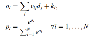
[math]\displaystyle{ \,o=Vh+k }[/math] where V is the weight matrix from hidden to output and k is another bias vector. [math]\displaystyle{ \,o }[/math] would be a vector with same dimensions as the total vocabulary size and the probabilities can be calculated from [math]\displaystyle{ \,o }[/math] by applying the softmax function.
The following figure shows the Architecture of the neural network language model. [math]\displaystyle{ \,h_j }[/math] denotes the context [math]\displaystyle{ \,w_{j-n+1}^{j-1} }[/math]. P is the size of one projection and H and N is the size of the second hidden and output layer, respectively. When short-lists are used the size of the output layer is much smaller than the size of the vocabulary.
In contrast to standard languaFile:Qq.pngge modeling where we want to know the probability of a word i given its context, [math]\displaystyle{ P(w_{j} = i|h_{j}) }[/math], the neural network simultaneously predicts the language model probability of all words in the word list:
Optimization and Training
The training was done with standard back-propagation on minimizing the error function:
[math]\displaystyle{ \,E=\sum_{i=1}^N t_i\ log p_i + \epsilon(\sum_{i,j}h^2_{ij}+\sum_{i,j}v^2_{ij}) }[/math]
[math]\displaystyle{ \,t_i }[/math] is the desired output vector and the summations inside the epsilon bracket are regularization terms to prevent overfitting of [math]\displaystyle{ \,H }[/math] and [math]\displaystyle{ \,V }[/math].
The researchers used stochastic gradient descent to prevent having to sum over millions of examples worth of error and this sped up training time.
An issue the researchers ran into using this model was that it took a long time to calculate language model probabilities compared to traditional back-off n-grams model and reduced its suitability for real time predictions. To solve this issue, several optimization techniques were used.
Lattice rescoring
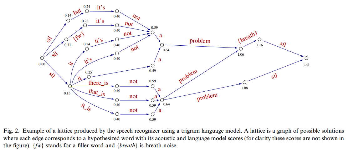
It is common to keep track of additional possible solutions instead of just the most obviously likely solution in a lattice structure, i.e. a tree like structure where branches can merge and each branch represents a possible solution. For example from the paper using a tri-gram model, i.e. predict third word from first two words, the following lattice structure was formed:
Any particular branch where two nodes have the same words can be merged. For example, "a,problem" was merged in the middle of the lattice because the tri-gram model would estimate the same probability at the point for both branch. Similary, "that_is,not" and "there_is,not" cannot be merged before the preceding two words to predict with are different.
After this structure is created with a traditional back-off n-grams model, the neural network is then used to re-score the lattice and the re-scored lattice is used to make predictions.
Short List
In any language, there is usually a small set of commonly used words that form almost all of written or spoken thought. The short-list idea is that rather than calculating every single probability for even the rarest words, the neural network only calculates a small subset of the most common words. This way, the output vector can be significantly shrunk from [math]\displaystyle{ \,\mbox{N} }[/math] to some much smaller number [math]\displaystyle{ \,\mbox{S} }[/math].
If any rare words do occur, their probabilities are calculated using the traditional back-off n-grams model. The formula then goes as follows from the paper:
Where L is the event that [math]\displaystyle{ \,w_t }[/math] is in the short-list.
Sorting and Bunch
The neural network predicts all the probabilities based on some sequence of words. If the probability of two different sequences of words are required but their relationship is such that for sequence 1, [math]\displaystyle{ \,w=(w_1,\dots,w_{i-1},w_i) }[/math] and sequence 2, [math]\displaystyle{ \,w^'=(w_1,\dots,w_{i-1},w^'_i) }[/math], they differ only in the last word. Then only a single feed through the neural network is required. This is because the output vector using the context [math]\displaystyle{ \,(w_1,\dots,w_{i-1}) }[/math] would predict the probabilities for both [math]\displaystyle{ \,w_i }[/math] and [math]\displaystyle{ \,w^'_i }[/math] being next. Therefore it is efficient to merge any sequence who have the same context.
Modern day computers are also very optimized for linear algebra and it is more efficient to run multiple examples at the same time through the matrix equations. The researchers called this bunching and simple testing showed that this decreased processing time by a factor of 10 when using 128 examples at once compared to 1.
Training and Usage
The researchers used numerous optimization techniques during training and their results were summarized in the paper as follows:
Since the model only trains to predict based on the last n-1 words, at certain points there will be less than n-1 words and adjustments must be made. The researchers considered two possibilities, using traditional models for these n-grams or filling up the n-k words with some filler word up to n-1. After some testing, they found that requests for small n-gram probabilities were pretty low and they decided to use traditional back-off n-gram model for these cases.
Results
In general the results were quite good. When this neural network + back-off n-grams hybrid was used in combination with a number of acoustic speech recognition models, they found that perplexity, lower the better, decreased by about 10% in a number of cases compared with traditional back-off n-grams only model. Some of their results are summarized as follows:
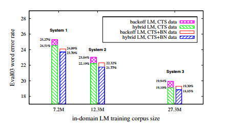
The following figure shows the word error rates on the 2003 evaluation test set for the back-off LM and the hybrid LM, trained only on CTS data (left bars for each system) and interpolated with the broadcast news LM (right bars for each system).
A perplexity reduction of about 9% relative is obtained independently of the size of the language model training data. This gain decreases to approximately 6% after interpolation with the back-off language model trained on the additional BN corpus of out-of domain data. It can be seen that the perplexity of the hybrid language model trained only on the CTS data is better than that of the back-off reference language model trained on all of the data (45.5 with respect to 47.5). Despite these rather small gains in perplexity, consistent word error reductions were observed.
Conclusion
This paper described the theory and an experimental evaluation of a new approach to language modeling for large vocabulary continuous speech recognition based on the idea to project the words onto a continuous space and to perform the probability estimation in this space. This method is fast to the level that the neural network language model can be used in a real-time speech recognizer. The necessary capacity of the neural network is an important issue. Three possibilities were explored: increasing the size of the hidden layer, training several networks and interpolating them together, and using large projection layers. Increasing the size of the hidden layer gave only modest improvements in word error, at the price of very long training times. In this respect, the second solution is more interesting as the networks can be trained in parallel. Large projection layers appear to be the best choice as this has little impact on the complexity during training or recognition.The neural network language model is able to cover different speaking styles, ranging from rather well formed speech with few errors (broadcast news) to very relaxed speaking with many errors in syntax and semantics (meetings and conversations). It is claimed that the combination of the developed neural network and a back-off language model can be considered as a serious alternative to the commonly used back-off language models alone.
This paper also proposes to investigate new training criteria for the neural network language model. Language models are almost exclusively trained independently from the acoustic model by minimizing the perplexity on some development data, and it is well known that improvements in perplexity do not necessarily lead to reductions in the word error rate.
The continuous representation of the words in the neural network language model offers new ways to perform constrained language model adaptation. For example, the continuous representation of the words can be changed so that the language model predictions are improved on some adaptation data, e.g., by moving some words closer together which appear often in similar contexts. The idea is to apply a transformation on the continuous representation of the words by adding an adaptation layer between the projection layer and the hidden layer. This layer is initialized with the identity transformation and then learned by training the neural network on the adaptation data. Several variants of this basic idea are possible, for example using shared block-wise transformations in order to reduce the number of free parameters. In comparison with back-off language models whose complexity increase exponentially with the length of context, complexity of neural network language models increase linearly with the order of the n-gram and with the size of the vocabulary. This linearly increase in parameters is an important practical advantage that enables us to consider longer span language models with a negligible increase of the memory and time complexity.
The underlying idea of the continuous space language model described here is to perform the probability
estimation in a continuous space. Although only neural networks were investigated in this work, the approach
is not inherently limited to this type of probability estimator. Other promising candidates include Gaussian
mixture models and radial basis function networks. These models are interesting since they can be more easily
trained on large amounts of data than neural networks, and the limitation of a short-list at the output may not
be necessary. The use of Gaussians makes it also possible to structure the model by sharing some Gaussians
using statistical criteria or high-level knowledge. On the other hand, Gaussian mixture models are a non-discriminative
approach. Comparing them with neural networks could provide additional insight into the success
of the neural network language model.
Source
Schwenk, H. Continuous space language models. Computer Speech Lang. 21, 492–518 (2007). ISIArticle


