a fair comparison of graph neural networks for graph classification
Presented By
Jaskirat Singh Bhatia
Background
Experimental reproducibility in machine learning has been known to be an issue for some time. Researchers attempting to reproduce the results of old algorithms have come up short, raising concerns that lack of reproducibility hurts the quality of the field. Lack of open source AI code has only exacerbated this, leading some to go so far as to say that "AI faces a reproducibility crisis" [1]. It has been argued that the ability to reproduce existing AI code, and making these codes and new ones open source is a key step in lowering the socio-economic barriers of entry into data science and computing. Recently, the graph representation learning field has attracted the attention of a wide research community, which resulted in a large stream of works. As such, several Graph Neural Network models have been developed to effectively tackle graph classification. However, experimental procedures often lack rigorousness and are hardly reproducible. The authors tried to reproduce the results from such experiments to tackle the problem of ambiguity in experimental procedures and the impossibility of reproducing results. They also Standardized the experimental environment so that the results could be reproduced while using this environment.
Graph Neural Networks
A graph is a data structure consisting of nodes and edges. Graph neural networks are models that take graph-structured data as input and capture information of the input graph, such as relation and interaction between nodes. In graph neural networks, nodes aggregate information from their neighbors. The key idea is to generate representations of nodes depending on the graph structure.
They provide a convenient way for node level, edge level, and graph level prediction task. The intuition of GNN is that nodes are naturally defined by their neighbors and connections. A typical application of GNN is node classification. Essentially, every node in the graph is associated with a label, and we want to predict the label of the nodes without ground-truth.
Graph neural networks can perform various tasks and have been used in many applications. Some simple and typical tasks include classifying the input graph or finding a missing edge/ node in the graph. One example of real applications where GNNs are used is social network prediction and recommendation, where the input data is naturally structural.
Graph basics
Graphs come from discrete mathematics and as previously mentioned are comprised of two building blocks, vertices (nodes), [math]\displaystyle{ v_i \in V }[/math], and edges, [math]\displaystyle{ e_j \in E }[/math]. The edges in a graph can also have a direction associated with them lending the name directed graph or they can be an undirected graph if an edge is shared by two vertices and there is no sense of direction. Vertices and edges of a graph can also have weights to them or really any amount of features imaginable.
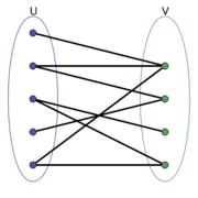
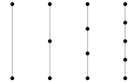
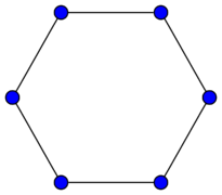
Now going one level of abstraction higher graphs can be categorized by structural patterns, we will refer to these as the types of graphs and this will not be an exhaustive list. A Bipartite graph (a) is one in which there are two sets of vertices [math]\displaystyle{ V_1 }[/math] and [math]\displaystyle{ V_2 }[/math] and there does not exist, [math]\displaystyle{ v_i,v_j \in V_k }[/math] where [math]\displaystyle{ k=1,2 }[/math] s.t. [math]\displaystyle{ v_i }[/math] and [math]\displaystyle{ v_j }[/math] share an edge, however, [math]\displaystyle{ \exists v_i \in V_1, v_j \in V_2 }[/math] where [math]\displaystyle{ v_i }[/math] and [math]\displaystyle{ v_j }[/math] share an edge. A Path graph (b) is a graph where, [math]\displaystyle{ |V| \geq 2 }[/math] and all vertices are connected sequentially meaning each vertex except the first and last have 2 edges, one coming from the previous vertex and one going to the next vertex. A Cycle graph (c) is similar to a path graph except each node has 2 edges and are connected in a loop, meaning if you start at any vertex and follow an edge of each node going in one direction it will eventually lead back to the starting node. These are just three examples of graph types in reality there are many more and it can beneficial to be able to connect the structure of ones data to an appropriate graph type.
-
(a) Bipartite Graph
-
(b) Path Graph
-
(c) Cycle Graph
Problems in Papers
Some of the most common reproducibility problems encountered in this field concern hyperparameters selection and the correct usage of data splits for model selection versus model assessment. Moreover, the evaluation code is sometimes missing or incomplete, and experiments are not standardized across different works in terms of node and edge features.
These issues easily generate doubts and confusion among practitioners that need a fully transparent and reproducible experimental setting. As a matter of fact, the evaluation of a model goes through two different phases, namely model selection on the validation set and model assessment on the test set. Clearly, to fail in keeping these phases well separated could lead to over-optimistic and biased estimates of the true performance of a model, making it hard for other researchers to present competitive results without following the same ambiguous evaluation procedures.
Risk Assessment and Model Selection
Risk Assessment
The goal of risk assessment is to provide an estimate of the performance of a class of models. When a test set is not explicitly given, a common way to proceed is to use k-fold Cross-Validation. As the model selection is performed independently for each training/test split, they obtain different “best” hyper-parameter configurations; this is why they refer to the performance of a class of models.
Model Selection
The goal of model selection, or hyperparameter tuning, is to choose among a set of candidate hyperparameter configurations the one that works best on a specific validation set. It also important to acknowledge the selection bias when selecting a model as this makes the validation accuracy of a selected model from a pool of candidates models a biased test accuracy.
Overview of Reproducibility Issues
The paper explores five different GNN models exploring issues with their experimental setup and potential reproducibility.
The GNN's were selected based on the following criteria
1. Performances obtained with 10-fold CV
2. Peer reviews
3. Strong architectural differences
4. Popularity
Criteria to assess the quality of evaluation and reproducibility was as follows
1. Code for data pre-processing
2. Code for model selection
3. Data splits are provided
4. Data is split by means of a stratification technique
5. Results of the 10-fold CV are reported correctly using standard deviations
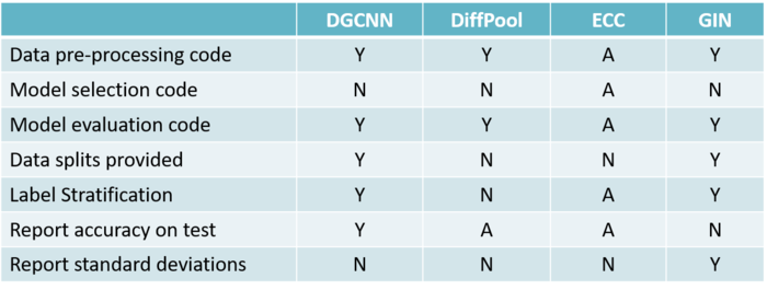
Using the following criteria, 4 different papers were selected and their assessment on the quality of evaluation and reproducibility is as follows:
Where (Y) indicates that the criterion is met, (N) indicates that the criterion is not satisfied, (A) indicates ambiguity (i.e. it is unclear whether the criteria is met or not), (-) indicates lack of information (i.e. no details are provided about the criteria).
Issues with DGCNN (Deep Graph Convolutional Neural Network)
The authors of DGCNN use a faulty method of tuning the learning rate and epoch. They used only a single fold for tuning hyperparameters despite evaluating the model on a 10-fold CV. This potentially leads to suboptimal performance. They haven't released the code for the experiments. Lastly, they average the one-fold CV across 10 folds and then report the numbers. This also reduces variance.
Issues with DiffPoll
It has not been clearly stated in the paper whether the results come from a test set or if they come from a validation set. Moreover, the standard deviation over the 10-fold CV has also not been reported. Due to no random seeds, different data splits are there while performing multi-fold splits (without stratification).
Issue with ECC
The results of the paper do not report the standard deviation obtained during the 10-fold Cross-Validation. Like in the case of GDCNN, the model selection procedure is not made clear due to pre-determined hyper-parameters. The code repository is not available as well.
Issues with GIN
Instead of reporting the test accuracy, the authors have given the validation accuracy over the 10-fold CV. Therefore, the given results are not suitable for evaluating the model. Code repository is not available for selecting the model.
Experiments
They re-evaluate the above-mentioned models on 9 datasets (4 chemical, 5 social), using a model selection and assessment framework that closely follows the rigorous practices as described earlier. In addition, they implemented two baselines whose purpose is to understand the extent to which GNNs are able to exploit structural information.
Datasets
All graph datasets used are publicly available (Kersting et al., 2016) and represent a relevant a subset of those most frequently used in literature to compare GNNs.
Features
In GNN literature, it is common practice to augment node descriptors with structural features. In general, good experimental practices suggest that all models should be consistently compared to the same input representations. This is why they re-evaluate all models using the same node features. In particular, they use one common setting for the chemical domain and two alternative settings as regards the social domain.
Baseline Model
They adopted two distinct baselines, one for chemical and one for social datasets. On all chemical datasets but for ENZYMES, they follow Ralaivola et al. (2005); Luzhnica et al. (2019) and implement the Molecular Fingerprint technique. On social domains and ENZYMES (due to the presence of additional features), they take inspiration from the work of Zaheer et al. (2017) to learn permutation-invariant functions over sets of nodes.
Experimental Setting
1. Used a 10-fold CV for model assessment and an inner holdout technique with a 90%/10% training/validation split for model selection.
2. After each model selection, they train three times on the whole training fold, holding out a random fraction (10%) of the data to perform early stopping.
3. The final test fold score is obtained as the mean of these three runs
4. To be consistent with the literature, they implemented early stopping with patience parameter n, where training stops if n epochs have passed without improvement on the validation set.
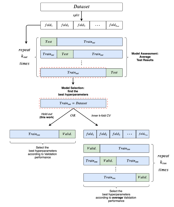
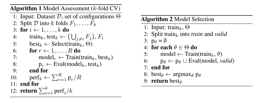
In order to better understand the Model Selection and the Model Assessment sections in the above figure, one can also take a look at the pseudo codes below.
Hyper-Parameters
1. Hyper-parameter tuning was performed via grid search.
2. They always included the hyper-parameters used by other authors in their respective papers.
Computational Considerations
As their research included a large number of training-testing cycles, they had to limit some of the models by:
1. For all models, grid sizes ranged from 32 to 72 possible configurations, depending on the number of hyper-parameters to choose from.
2. Limited the time to complete a single training to 72 hours.
Effect of Node Degree on Layering
The above table displays the median number of selected layers in relation to the addition of node degrees as input features on all social datasets. 1 indicates that an uninformative feature is used as a node label.
Comparison with Published Results
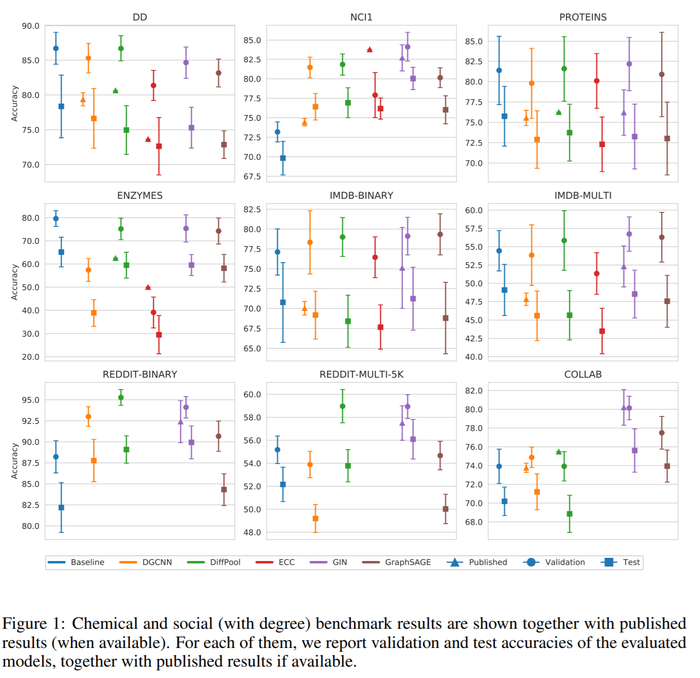
In the above figure, we can see the comparison between the average values of test results obtained by the authors of the paper and those reported in the literature. In addition to that, the validation results across the 10 different model selections were plotted. The plots show how the test accuracies calculated in this paper are in most cases different from what reported in the literature, and the gap between the two estimates is usually consistent. Also, the average validation accuracies calculated by the authors are always higher or equal to the test results.
Source Codes
The data and scripts to reproduce the experiments reported in the paper are available at https://github.com/diningphil/gnn-comparison .
Conclusion
1. Highlighted ambiguities in the experimental settings of different papers
2. Proposed a clear and reproducible procedure for future comparisons
3. Provided a complete re-evaluation of four GNNs
4. Found out that structure-agnostic baselines outperform GNNs on some chemical datasets, thus suggesting that structural properties have not been exploited yet.
Critique
This paper raises an important issue about the reproducibility of some important 5 graph neural network models on 9 datasets. The reproducibility and replicability problems are very important topics for science in general and even more important for fast-growing fields like machine learning. The authors proposed a unified scheme for evaluating reproducibility in graph classification papers. This unified approach can be used for future graph classification papers such that the comparison between proposed methods becomes clearer. The results of the paper are interesting as in some cases the baseline methods outperform other proposed algorithms. Finally, I believe one of the main limitations of the paper is the lack of technical discussion. For example, this was a good idea to discuss in more depth why baseline models are performing better? Or why the results across different datasets are not consistent? Should we choose the best GNN based on the type of data? If so, what are the guidelines?
Also as well known in the literature of GNNs that they are designed to solve the non-Euclidean problems on graph-structured data. This is kinds of problems are hardly be handled by general deep learning techniques and there are different types of designed graphs that handle various mechanisms i.e. heat diffusion mechanisms. In my opinion, there would a better way to categorize existing GNN models into spatial and spectral domains and reveal connections among subcategories in each domain. With the increase of the GNNs models, further analysis must be handled to establish a strong link across the spatial and spectral domains to be more interpretable and transparent to the application.
References
- Davide Bacciu, Federico Errica, and Alessio Micheli. Contextual graph Markov model: A deep and generative approach to graph processing. In Proceedings of the International Conference on Machine Learning (ICML), volume 80 of Proceedings of Machine Learning Research, pp. 294–303. PMLR, 2018.
- Paul D Dobson and Andrew J Doig. Distinguishing enzyme structures from non-enzymes without alignments. Journal of molecular biology, 330(4):771–783, 2003.
- Will Hamilton, Zhitao Ying, and Jure Leskovec. Inductive representation learning on large graphs. In Advances in Neural Information Processing Systems (NIPS), pp. 1024–1034. Curran Associates, Inc., 2017.
- Kristian Kersting, Nils M. Kriege, Christopher Morris, Petra Mutzel, and Marion Neumann. Benchmark data sets for graph kernels, 2016. URL http://graphkernels.cs.tu-dortmund. de.
- Muhan Zhang and Yixin Chen. Link prediction based on graph neural networks. In Advances in Neural Information Processing Systems (NeurIPS), pp. 5165–5175. Curran Associates, Inc., 2018.
[1] Hutson, M. (2018). Artificial intelligence faces a reproducibility crisis. Science, 359(6377), 725–726.
