Unsupervised Learning of Optical Flow via Brightness Constancy and Motion Smoothness
Presented by
- Hudson Ash
- Stephen Kingston
- Alexandre Xiao
- Richard Zhang
- Ziqiu Zhu
Problem & Motivation
The approaches to solving optimal flow problems, albeit widely successful, has mostly been a result of supervised learning methods using convolutional neural networks (convnets). The inherent challenge with these supervised learning approaches lies in the groundtruth flow, the process of gathering provable data for the measure of the target variable for the training and testing datasets. Directly obtaining the motion field groundtruth from real life videos is not possible, but instead, synthetic data is often used.
The paper "Back to Basics: Unsupervised Learning of Optical Flow via Brightness Constancy and Motion Smoothness" by Yu et. al. presents an unsupervised approach to address the groundtruth acquisition challenges of optical flow, by making use of the standard Flownet architecture with a spatial transformer component to devise a "self-supervising" loss function.
Optical Flow
Optical flow is the apparent motion of image brightness patterns in objects, surfaces and edges in videos. In more laymen terms, it tracks the change in position of pixels between two frames caused by the movement of the object or the camera. Most optical flows are estimated on the basis of two assumptions:
1. Pixel intensities do not change rapidly between frames (brightness constancy).
2. Groups of pixels move together (motion smoothness).
Both of these assumptions are derived from real-world implications. Firstly, the time between two consecutive frames of a video are so minuscule, such that it becomes extremely improbable for the intensity of a pixel to completely change, even if its location has changed. Secondly, pixels do not teleport. The assumption that groups of pixels move together implies that there is spatial coherence and that the image motion of objects changes gradually over time, creating motion smoothness.
Given these assumptions, imagine a video frame (which is 2D image) with a pixel at position [math]\displaystyle{ (x,y) }[/math] at some time t, and in later frame, the pixel is now in position [math]\displaystyle{ (x + \Delta x, y + \Delta y) }[/math] at some time [math]\displaystyle{ t + \Delta t }[/math].
Then by the first assumption, the intensity of the pixel at time t is the same as the intensity of the pixel at time [math]\displaystyle{ t + \Delta t }[/math]:
- [math]\displaystyle{ I(x+\Delta x,y+\Delta y,t+\Delta t) = I(x,y,t) }[/math]
Using Taylor series, we get:
- [math]\displaystyle{ I(x+\Delta x,y+\Delta y,t+\Delta t) = I(x,y,t) + \frac{\partial I}{\partial x}\Delta x+\frac{\partial I}{\partial y}\Delta y+\frac{\partial I}{\partial t}\Delta t }[/math], ignoring the higher order terms.
From the two equations, it follows that:
- [math]\displaystyle{ \frac{\partial I}{\partial x}\Delta x+\frac{\partial I}{\partial y}\Delta y+\frac{\partial I}{\partial t}\Delta t = 0 }[/math]
which results in
- [math]\displaystyle{ \frac{\partial I}{\partial x}V_x+\frac{\partial I}{\partial y}V_y+\frac{\partial I}{\partial t} = 0 }[/math]
where [math]\displaystyle{ V_x,V_y }[/math] are the [math]\displaystyle{ x }[/math] and [math]\displaystyle{ y }[/math] components of the velocity (displacement over time) or optical flow of [math]\displaystyle{ I(x,y,t) }[/math] and [math]\displaystyle{ \tfrac{\partial I}{\partial x} }[/math], [math]\displaystyle{ \tfrac{\partial I}{\partial y} }[/math], and [math]\displaystyle{ \tfrac{\partial I}{\partial t} }[/math] are the derivatives of the image at [math]\displaystyle{ (x,y,t) }[/math] in the corresponding directions.
This can be rewritten as:
- [math]\displaystyle{ I_xV_x+I_yV_y=-I_t }[/math]
or
- [math]\displaystyle{ \nabla I^T\cdot\vec{V} = -I_t }[/math]
Where [math]\displaystyle{ \nabla I^T }[/math] is known as the spatial gradient
Since this results in one equation with two unknowns [math]\displaystyle{ V_x,V_y }[/math], it results into what is known as the aperture problem of the optical flow algorithms. In order to solve the optical flow problem, another set of constraints are required, which is where assumption 2 can be applied.
Traditional Approaches
Traditional approaches to the optical flow problem consisted of many differential (gradient-based) methods. Horn and Schunck, 1981, being one of the first to create an approach for for optical flow estimation, is one of the classical examples for optical flow estimation. Without diving deep into the math, Horn and Schunk created constraints based on spatio-temporal derivatives of image brightness. Their estimation tries to solve the aperture problem by adding a smoothness condition where that the optical flow field varies smoothly through the entire image (a global motion smoothness). They assume that object motion in a sequence will be rigid and approximately constant, that the objects in a pixel’s neighborhood will have similar velocities, and therefore the object changes smoothly over space and time. The challenges with this approach is that on frames with rougher movements, the accuracy of the estimates dramatically decrease.
Another classical method, Lucas-Kanade, approaches the problem by taking a local motion smoothness assumption. Lucas-Kanade addressed the sensitivity to rough movements in the Horn and Schunk approach by making a local motion smoothness assumption instead of a global motion smoothness. While the Lucas-Kanade estimation reduced sensitivity to rougher movements, it still has inaccuracy in rough frames as a differential method to optical flow estimation.
In 2015, FlowNet was proposed as the first approach to use a deep neural network for end-to-end optical flow estimation.
Related Works
FlowNet: Supervised Optical Flow
FlowNet Architecture
Convolutional Neural Networks have been at the forefront of image classification since its inception in 1994. However, a neural network was not created for supervised optical flow until 2015. This is due to the large quantities of labeled training data required to train an accurate CNN. In order to apply a neural network, the FlowNet team had to create their own artificial training data, the flying chair dataset.
FlowNet comes in two variations: FlowNetSimple and FlowNetCorrelation.
FlowNet Simple
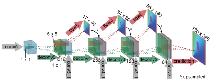
FlowNetSimple is a standard CNN. It layers two images on top of one another, resulting in 6 channels (3 RBG channels for each image). It then applies nine convolution layers, starting with a large 7x7 filter with a stride of 2. It nearly doubles the number of feature maps with each iteration, until the final step of a 6x8 image with 1024 feature maps. The image then goes through up-convolution refinement (as seen below) and predicts the optical flow between two images.
FlowNet Correlation
FlowNetCorr extracts features from each image independently for the first three convolution layers. It then finds the correlation between each "patch" of image 1 and each "patch" of image 2. The feature maps are then replaced with correlation values. To reduce computational intensity, correlations with displacement D are only calculated, meaning only nearby patches are calculated for correlation. FlowNetCorr is similar to FlowNetSimple in the later half of the network.
FlowNet Refinement Process
The refinement process up-convolutes the images. By the time it reaches the ninth convolutional layer, the image is reduced to 1024 6x8 representations. This does not give us enough comparison to the known optical flow, therefore the image's resolution is increased. Each pixel in the 6x8 is mapped to a 5x5 square for half the number of feature maps. The image's previously trained 512 feature maps from the 7th convolutional network are concatenated onto the expanded feature maps, and the process is repeated 4 times until the image resolution is 4x smaller than the input size. It is found that expanding the image beyond this size does not improve performance.
Training Data
At the time, the standard optical flow dataset for supervised learning was the KITTI dataset. The KITTI dataset was created for many computer vision benchmarks: 3D object detection, 3D tracking, and optical flow. The data was collected by driving a car around a mid-sized German town which gave many data points, but resulted in a very specific type of flow that was hard to generalize to other forms of optical flow. Its main drawback was its small size of only 194 frame pairs, which proved to be insufficient for accurately training a convolutional neural network.
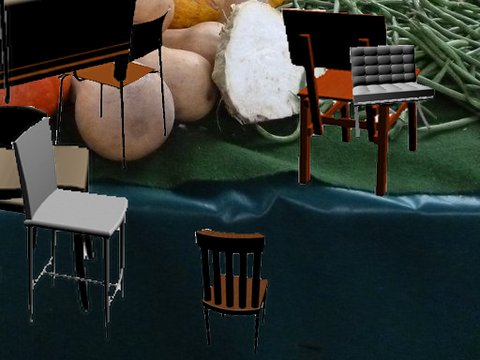
As a result, a "flying chair" dataset was created in order to train the network. 22,872 image pairs were created. The first image samples Flickr for a random background of a mountain, city, or landscape and a 3D chair model dataset superimposed in the foreground. Affine transformations are applied to the chairs and background to create a second image that simulates motion. The groundtruth flow is derived from the transformations. All potential variables of each image (number of chairs, sizes of chairs, etc.) are randomly sampled from a distribution that matches the Sintel dataset, another popular optical flow training option.
Spatial Transformer Networks
As Convolutional Neural Networks have been established as the preferred solution in image recognition and computer vision problems, increasing attention has been dedicated to evolving the network architecture to further improve predictive power. One such adaptation is the Spatial Transformer Network, developed by Google DeepMind in 2015.
Spacial invariance is a desired property of any system that deals with visual task, however the basic CNN is not very robust in the presence of input deformations such as scale/translation/rotation variations, viewpoint variations, shape deformations, etc. The introduction of local pooling layers into CNNs have helped address this issue to some degree, by pooling groups of input cells into simpler cells, helping to remove the adverse impact of noise on the input. However, pooling layers are destructive - a standard 2x2 pooling layer discards 75% of the input data, resulting in the loss of exact positional data, which can be very helpful visual recognition tasks. Also, since pooling layers are predefined and non-adaptive, their inclusion may only be helpful in the presence of small deformations; with large transformations, pooling may help provide little to no spatial invariance to the network.
The Spatial Transformer Network (STN) addresses the spatial invariance issues described above by producing an explicit spatial transformation to carve out the target object. Advantageous properties of the STN are as follows:
1. Modular - they can easily be implemented anywhere into an existing CNN
2. Differentiable - they can be trained using backpropagation without modifying the original model
3. Dynamic - they perform a unique spatial transformation on the feature map for each input sample
STNs are composed of three primary components:
1. Localization network: a CNN that outputs the parameters of a spatial transformations
2. Grid Generator: Generates a sampling grid, where transformations from the localization network are applied to this grid
3. Sampler: Samples the input feature map according to the transformed grid and a differentiable interpolation function
The Paper's Approach: UnsupFlownet
Architecture
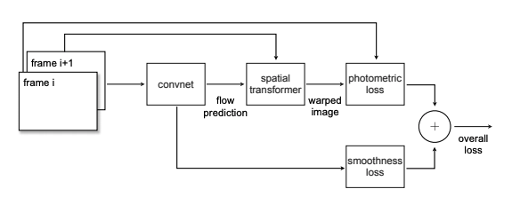
UnsupFlownet's architecture uses Flownet Simple as the core component for optical flow estimation. Two consecutive frames are inputted into the Flownet component. The estimated flow is then inputted to the spatial transformer unit to warp the second frame into the first frame. The spatial transformer performs the following pointwise transformation:
[math]\displaystyle{ \begin{bmatrix} x_2 \\ y_2 \end{bmatrix} = \begin{bmatrix} x_1 + u \\ x_2 + v \end{bmatrix} }[/math],
where [math]\displaystyle{ (x_1, y_1) }[/math] are the coordinates in the first frame, and [math]\displaystyle{ (x_2, y_2) }[/math] are the sampling coordinates in the second frame, and [math]\displaystyle{ (u, v) }[/math] is the estimated flow in the horizontal and vertical components, respectively.

Due to the spatial transformer's differentiable nature, the gradients of the losses can be successfully back-propagated to the convnet weights, thereby training the network.
Unsupervised Loss
The paper devises the following loss function:
[math]\displaystyle{ \mathcal{L}(\mathbf{u}, \mathbf{v}; I_t, I_{t+1}) = l_{photometric}(\mathbf{u}, \mathbf{v}; I_t, I_{t+1}) + \lambda l_{smoothness}(\mathbf{u}, \mathbf{v}) }[/math]
where [math]\displaystyle{ (\mathbf{u}, \mathbf{v}) }[/math] is the estimated flow, and [math]\displaystyle{ I_t(\cdot, \cdot), I_{t+1}(\cdot, \cdot) }[/math] are the photo-intensity (RGB) functions at frame [math]\displaystyle{ t }[/math] and frame [math]\displaystyle{ t + 1 }[/math], respectively. The photo-intensity functions accept an [math]\displaystyle{ (x, y) }[/math] coordinate and returns the RGB values at that pixel.
Photo Constancy
The photometric term is defined as:
[math]\displaystyle{ l_{photometric}(\mathbf{u}, \mathbf{v}; I_t, I_{t+1}) = \sum\limits_{i,j}\rho_D\Big(I_t(i, j) - I_{t+1}(i + u_{i,j}, j + v_{i,j})\Big) }[/math]
where [math]\displaystyle{ \rho_D }[/math] is some robust penalty function taking on the form [math]\displaystyle{ (x^2 + \epsilon^2)^{\alpha}, 0 \lt \alpha \lt 1 }[/math].
This term addresses the first assumption in Section 3. We have that if the estimated flow [math]\displaystyle{ (\mathbf{u}, \mathbf{v}) }[/math] is correct, then the reconstructed (warped) second frame should very closely resemble the first frame. Hence, the photometric loss would be low. The opposite is true for poor flow estimation.
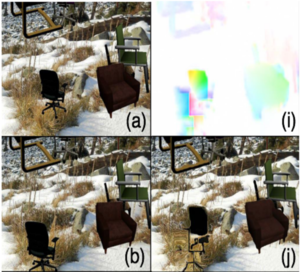
Below is an example of warping. Panels (a) and (b) are the first and second frame respectively, (i) is the estimated flow, and (j) is the second frame warped by (i).

Local Smoothness
The smoothness term is defined as:
[math]\displaystyle{ l_{smoothness}(\mathbf{u}, \mathbf{v}) = \sum\limits_j^H\sum\limits_i^W \Big(\rho_S(u_{i,j}, u_{i+1, j}) + \rho_S(u_{i,j} - u_{i, j+1}) + \rho_S(v_{i,j} - v_{i+1, j}) + \rho_S(v_{i,j} - v_{i,j+1})\Big) }[/math]
This term addresses the second assumption in Section 3. It computes a robust penalty, [math]\displaystyle{ \rho_S(\cdot) }[/math], of the difference between the estimated flow of each pixel and that of its nearest rightward and upward neighbour. This penalizes local non-smoothness. The robustness of the penalty function is important, since we expect that at object boundaries, optical flow should change drastically. Therefore, there should be expected large differences in certain spots in the frame. The penalty would still penalize this difference, but avoids generating a large gradient with respect to the flow, by levelling off at large [math]\displaystyle{ x }[/math]-axis values.

Results & Future Work
Two data sets were used to validate the model and test its performance, namely Flying Chairs and KITTI 2012.
Flying Chairs
The flying chairs data set is an artificially constructed set of motion images. They consist of a still colour background image and a sequence of 3D modeled chairs moving across the screen. The dataset contains 22,232 training and 640 test image pairs with groundtruth flow. The benefit to the generated nature of this data set is it has a corresponding 'class' associated with each image. This makes supervised methods much more accurate, but is an unrealistic approach for real life applications where groundtruth flow is unavailable.

KITTI 2012
The KITTI data set consists of videos from cameras mounted above vehicles, driving through various roads and highways. The data set is smaller than the flying chairs set and contains no prexisting groundtruth flow. This data set is much more indicative of real world applications as it is often difficult to have true representations of output for which to train and validate supervised learning techniques.


