Pixels to Graphs by Associative Embedding
Introduction
Extracting semantics from images is one of the main goals of computer vision. Recent years have seen rapid progress in the classification and localization of objects [7, 24, 10]. But a bag of labeled and localized objects is an impoverished representation of image semantics: it tells us what and where the objects are (“person” and “car”), but does not tell us about their relations and interactions (“person next to car”). A necessary step is thus to not only detect objects but to identify the relations between them. An explicit representation of this semantics is referred to as a scene graph where we represent objects grounded in the scene as vertices and the relationships between them as edges. [1]
End-to-end training of convolutional networks has proven to be a highly effective strategy for image understanding tasks. It is therefore natural to ask whether the same strategy would be viable for predicting graphs from pixels. Existing approaches, however, tend to break the problem down into more manageable steps. For example, one might run an object detection system to propose all of the objects in the scene, then isolate individual pairs of objects to identify the relationships between them. This breakdown often restricts the visual features used in later steps and limits reasoning over the full graph and over the full contents of the image. [1]
The paper presents a novel approach to generating a scene graph. A scene graph, as it relates to an image, is a graph with a vertex that represents each object identified in the image and an edge that represents relationships between the objects.
An example of a scene graph:
Current state-of-the-art techniques break down the construction of scene graphs by first identifying objects and then predicting the edges for any given pair of identified objects. By using this technique, reasoning over the full graph would be limited. On the other hand, this paper introduces an architecture that defines the entire graph directly from the image, enabling the network to reason across the entirety of the image to understand relationships, as opposed to only predicting relationships using object labels.
A key concern, given that the new architecture produces both vertices (objects) and edges (relationships), is connecting the two. Specifically, the output of the network is some set of relationships E, and some set of vertices V. The network needs to also output the “source” and “destination” of each relationship so that the final graph can be formed. In the image above, for example, the network would also need to tell us that “holding” comes from “person” and goes to “Frisbee”. To do this, the paper uses associative embeddings. Specifically, the network outputs a particular “embedding vector” for each vertex, as well as a “source embedding” and “destination embedding” for each relationship. A final post-processing step finds the vertex embedding closest to each of the source/destination embeddings of each relationship and in this way assigns the edges to pairs of vertices.
Previous Work
Relationship detection
Relationship detection aims at correctly determining the relationships between pairs of objects and ground that is in the image with accurate object bounding boxes. Visual relationship is the center of attraction recently. Since the task itself is open-ended and challenging, it leads to variety of diverse approaches and solutions.
In the field of relationship detection, the following are the existing state of the art advances:
1) Framing the task of identifying objects using localization from referential expressions, detection of human-object interactions, or the more general tasks of Visual Relationship Detection (VRD) and scene graph generation.
2) Visual relationship detection methods like message passing RNNs and predicting over triplets of bounding boxes.
Associative Embedding
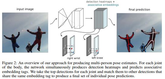
There are various contexts where associative embedding are used. To take an example they are used to measure the similarity between pairs of images. Recently vector embedding have been used to group together body joints for multi-person pose estimation. These are referred to as associative embeddings since supervision does not require the network to output a particular vector value, and instead uses the distances between pairs of embedding to calculate a loss. The important thing is no the exact value of the vector but how it relates to the other embedding produced by the network.
In the field of associative embedding, the following are some interesting applications:
1) Vector embeddings to group together body joints for multi-person pose estimation.
2) Vector embeddings to detect body joints of the various people in an image.
Reference Figure from the paper "Associative embedding: End-to-end learning for joint detection and grouping."

Pixels To Graphs
The goal of the paper is to construct a graph from a set of pixels. In particular, to construct a graph grounded in the space of these pixels. Meaning that in addition to identifying vertices of the graph, we want to know their precise locations. A vertex, in this case, can refer to any object of interest in the scene including people, cars, clothing, and buildings. The relationships between these objects is then captured by the edges of the graph. These relationships may include verbs (eating, riding), spatial relations (on the left of, behind), and comparisons (smaller than, same color as).
Formally we consider a directed graph G = (V, E). A given vertex vi ∈ V is grounded at a location ([math]\displaystyle{ xi }[/math] ,[math]\displaystyle{ yi }[/math]) and defined by its class and bounding box. Each edge e ∈ E takes the form ei = ([math]\displaystyle{ vs }[/math],[math]\displaystyle{ vt }[/math] ,[math]\displaystyle{ ri }[/math]) defining a relationship of type [math]\displaystyle{ r_i }[/math] from [math]\displaystyle{ vs }[/math] to [math]\displaystyle{ vt }[/math] . We train a network to explicitly define V and E. This training is done end-to-end on a single network, allowing the network to reason fully over the image and all possible components of the graph when making its predictions
The Architecture:
- 1. Detecting Graph Elements
Given an image of dimensions h x w, a stacked hourglass (Appendix 2) is used to generate a h x w x f representation of the image. It should be noted that the dimension of the output (which is non-trainable), needs to fulfill certain criteria. Specifically, we need to have a resolution large enough to minimize the number of pixels with multiple detections while also being small enough to ensure that each 1 x 1 x f vector still contains the information needed for subsequent inference.
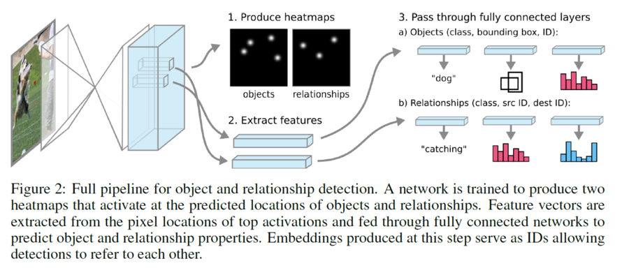
A 1x1 convolution and sigmoid activation is performed on this result to generate a heat map (one for objects and one for relationships, using separately determined convolutions). The value at a given pixel can be interpreted as the likelihood of detection at that particular pixel in the original image.
In order to claim that there is an element at some pixel, we need to have some likelihood threshold. Then, if a given pixel in the map has a value >= the threshold, we claim that there is an element at that pixel. This threshold is calculated by using binary cross-entropy loss on the final values in the heat map. Values with likelihoods greater than p-hat will be considered element detections.
Finally, for each element that we detected, we extract the 1 x 1 x f feature vector. This is then used as an input to a set of Feed Forward Neural Networks (FFNNs), where we have a separate network for each characteristic of interest, and for each network, there's one hidden layer with f nodes. The object class and relationship (edges) could be supervised by softmax loss. Furthermore, in order to predict the bounding box of the object, we can use the approach proposed by the Faster-RCNN model[3]. The following image summarizes the process.

- 2. Connecting Elements with Associative Embeddings
As explained earlier, to construct the scene graph, we need to know the source and destination of each edge. This is done through associative embeddings.
First, let us define an embedding hi ϵ Rd produced for some vector i, and let us assume that we have n object detections in a particular image. Now, define hik, for k = 1 to Ki (where Ki is the number of edges in the graph with a vertex at vertex i) as the embedding associated with an edge that touches vertex i. We define two loss functions on these sets.
The goal of Lpull is to minimize the squared differences between the embedding of a given vertex and the embedding of an edge that references said vertex.
On the other hand, minimizing Lpush implies assigning embeddings to vertices that are as far apart as possible. The further apart they are, the lower the output of max becomes until eventually, it reaches 0. Here, m is just a constant. In the paper, the values used were m = 8 and d = 8 (that is, 8D embeddings). Combining these two loss functions (and weighing them equally), accomplishes the task of predicting embeddings such that vertices are differentiated, but the embedding of a vertex is most similar to the vertex it references.
- 3. Support for Overlapping Detections
An obvious concern is how the network would operate if there was more than one detection (be it object or relationship), in a given pixel. For example, detection of “shirt” and “person” may be centered at the exact same pixel. To account for this, the architecture is modified to allow for “slots” at each pixel. Specifically, so detections of objects are allowed at a particular pixel, while sr relationship detections are allowed at a given pixel.
In order to allow for this, some changes are required after the feature extraction step. Specifically, we now use the 1x1xf vector as the input for so (or sr) different sets of 4 FFNNs, where the output (of the first three) is as shown in figure 2, and with the final FFNN outputting the probability of a detection existing in that particular slot, at that particular pixel. This new network is trained exclusively on whether or not a detection has been made in that slot, and, in prediction, is used to determine the number of slots to output at a given pixel. It is critical to note that this each of these so (or sr) sets of FFNNs share absolutely no weights. And each is trained for detection in its assigned slot.
It is important to note that this implies a change in the training procedure. We now have so (or sr) different predictions (be it class, or class + bounding box), that we need to match with our set of ground truth detections at a given pixel. Without this step, we would not be able to assign a value to the error for that sample. To do this, we match a one-hot encoded vector of the ground-truth class and bounding box anchor (the reference vector), and then match them with the so (or sr) outputs provided at a given pixel. The Hungarian method is used to ensure maximum matching between the outputs and the reference method while ensuring we do not assign the same detection to multiple slots.
Results
A quick note on notation: R@50 indicates what percentage of ground-truth subject-predicate-object tuples appeared in a proposal of 50 such tuples. Since R@100 offers more possibilities, it will necessarily be higher. The 6.7, for example, indicates that 6.7% of the ground truth tuples appeared in the proposals of the network.
The authors tested the network against two other architectures designed to develop a semantic understanding of images. For this, they used the Visual Genome dataset, with so = 3 and sr = 6. Overall, the new architecture vastly outperformed past models. The results were as follows:
The table can be interpreted as follows:

- SGGen (no RPN): Given a particular image, without the use of Region Proposal networks, the accuracy of the proposed scene graph. No class predictions are provided.
- SGGen (with RPN): Same as above, except the output of the Region Proposal Network, is used to enhance the input of a given image. No class predictions are provided.
- SGCIs: Ground-truth object bounding boxes are provided. The network is asked to classify them and determine relationships.
- PredCIs: As above, except the classes are also provided. The only goal is to predict relationships.
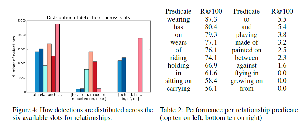
Further analysis into the accuracy, when looking at predicates individually, shows that the architecture is very sensitive to over-represented relationship predicates.
As shown in Figure 5, for many ground-truth predicates (those that do not appear often in the ground truth), the network does poorly. Even when allowed to propose 100 tuples, the network does not offer the predicate. Figure 4 simply observes the fact that certain sets of relationship predicates appear predominantly in a subset of slots. No general explanation has been offered for this behavior.
Conclusion
In conclusion, the paper offers a novel approach that enables the extraction of image semantics while perpetually reasoning over the entire context of the image. Associative embeddings are used to connect object and predicate relationships, and parallel “slots” allow for multiple detections in one pixel. While this approach offers noticeable improvements in accuracy, it is clear that work needs to be done to account for the non-uniform distributions of relationships in the dataset.
Critiques
The paper's contributions towards patterning unordered network outputs and using associative embeddings for connecting vertices and edges are commendable. However, it should be noted this paper is only an incremental improvement over existing well-studied architectures like the hourglass architecture. The modifications are not sufficiently supported by mathematical reasoning. The authors say that they make a slight modification to the hourglass design and double the number of features and weight all the loses equally. No scientific justification for why this is needed is given. Also the choice of constants to be 3 and 6 for [math]\displaystyle{ s_o }[/math] and [math]\displaystyle{ s_r }[/math] is not clear, as the authors leave out a fraction of the cases. I am not sure if the changes made are truly a critical advance as the experiments are conducted only on a single dataset and no generalizability arguments are made by the authors. So the methods might just work well only for this dataset and the changes may pertain to only this one. The theoretical analysis done in the paper comes directly from the hourglass literature and cannot be accounted for novelty. The paper could have identified the effect of their treatment by analyzing the structure of the network that they are presenting. However, there are lack of mathematical and structural analysis of each treatment that they are presenting in detailed levels.
Appendices
Appendix 1: Sample Outputs
Appendix 2: Stacked Hourglass Architecture
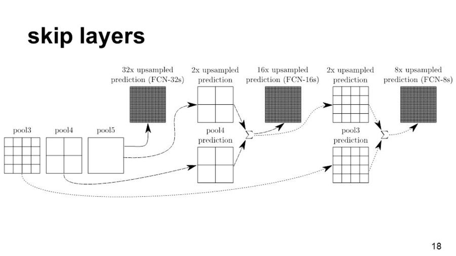
Although this goes beyond the focus of the paper, I would like to add a brief overview of the stacked hourglass architecture used to generate the heat map. This architecture is unique in that it allows cyclical top-down, bottom-up inference and recombination of features. While most architectures focus on optimizing the bottom-up portion (reducing dimensionality), the stacked-hourglass gives the network more flexibility in how it generates a representation by allowing it to learn a series of down-sampling / up-sampling steps.
When you downsample and then upsample, a high amount of information is potentially lost on the upsampled reconstruction. Using the naive approach, this often results in poor reconstruction. This problem is accentuated when we stack multiple layers of downsampling and upsampling in the stacked hourglass architecture. To alleviate this issue, we add skip layers. Skip layers essentially allow earlier layers to send outputs into multiple later layers. The added information from the earlier layers ensures that the reconstructed embedding doesn't have its dimensionality reduced too much.

References
1. Alejandro Newell and Jia Deng, “Pixels to Graphs by Associative Embedding,” in NIPS, 2017. URL https://arxiv.org/abs/1706.07365
2. Alejandro Newell, Kaiyu Yang, and Jia Deng. Stacked Hourglass Networks for Human Pose Estimation. ECCV, 2016. URL https://arxiv.org/abs/1603.06937
3. Shaoqing Ren, Kaiming He, Ross Girshick, and Jian Sun. Faster r-cnn: Towards real-time object detection with region proposal networks. NIPS, pages 91–99, 2015. URL https://arxiv.org/abs/1506.01497


