Patch Based Convolutional Neural Network for Whole Slide Tissue Image Classification

Presented by

Cassandra Wong, Anastasiia Livochka, Maryam Yalsavar, David Evans

Introduction

Despite the fact that CNN are well-known for their success in image classification, it is computationally impossible to use them for cancer classification. This problem is due to high-resolution images that cancer classification is dealing with. As a result, this paper argues that using a patch level CNN can outperform an image level based one and considers two main challenges in patch level classification – aggregation of patch-level classification results and existence of non-discriminative patches. For dealing with these challenges, training a decision fusion model and an Expectation-Maximization (EM) based method for locating the discriminative patches are suggested respectively. At the end the authors proved their claims and findings by testing their model to the classification of glioma and non-small-cell lung carcinoma cases.

Previous Work

The proposed patch-level CNN and training a decision fusion model as a two-level model was made apparent by the various breakthroughs and results noted below:

Majority of Whole Slide Tissue Images classification methods fixate on classifying or obtaining features on patches [1, 2, 3]. These methods excel when an abundance of patch labels are provided [1, 2], allowing patch-level supervised classifiers to learn the assortment of cancer subtypes. However, labeling patches requires specialized annotators; an excessive task at a large scale.
Multiple Instance Learning (MIL) based classification [4, 5] utilizes unlabeled patches to predict a label of a bag. For a binary classification problem, the main assumption (Standard Multi-Instance assumption, SMI) states that a bag is positive if and only if there exists at least one positive instance in the bag. Some authors combine MIL with Neural Networks[6, 7] and model SMI by max-pooling. This approach is inefficient due to only one instance with a maximum score (because of max-pooling) being trained in one training iteration on the entire bag.
Other works sometimes apply average pooling (voting). However, it has been shown that many decision fusion models can outperform simple voting[8, 9]. The choice of the decision fusion function would depend heavily on the domain.

EM-based Method with CNN

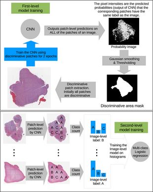
The high-resolution image is modelled as a bag, and patches extracted from it are instances that form a specific bag. The ground truth labels are provided for the bag only, so we model the labels of an instance (discriminative or not) as a hidden binary variable. Hidden binary variables are estimated by the Expectation-Maximization algorithm. A summary of the proposed approach can be found in Fig.2. Please note that this approach will work for any discriminative model.

In this paper [math]\displaystyle{ X = \{X_1, \dots, X_N\} }[/math] denotes dataset containing [math]\displaystyle{ N }[/math] bags. A bag [math]\displaystyle{ X_i= \{X_{i,1}, X_{i,2}, \dots, X_{i, N_i}\} }[/math] consists of [math]\displaystyle{ N_i }[/math] pathes (instances) and [math]\displaystyle{ X_{i,j} = \lt x_{i,j}, y_j\gt }[/math] denotes j-th instance and it’s label in i-th bag. We assume bags are i.i.d. (independent identically distributed), [math]\displaystyle{ X }[/math] and associated hidden labels [math]\displaystyle{ H }[/math] are generated by the following model: $$P(X, H) = \prod_{i = 1}^N P(X_{i,1}, \dots , X_{i,N_i}| H_i)P(H_i) \quad \quad \quad \quad (1) $$ [math]\displaystyle{ Hi = {H_{i, 1}, \dots, H_{i, Ni}} }[/math] denotes the set of hidden variables for instances in the bag [math]\displaystyle{ X_i }[/math] and [math]\displaystyle{ H_{i, j} }[/math] indicates whether the patch [math]\displaystyle{ X_{i,j} }[/math] is discriminative for [math]\displaystyle{ y_i }[/math] (it is discriminative if estimated label of the instance coincides with the label of the whole bag). Authors assume that [math]\displaystyle{ X_{i, j} }[/math] is independent from hidden labels of all other instances in the i-th bag, therefore [math]\displaystyle{ (1) }[/math] can be simplified as: $$P(X, H) = \prod_{i = 1}^{N} \prod_{j=1}^{N_i} P(X_{i, j}| H_{i, j})P(H_{i, j}) \quad \quad (2)$$ Authors propose to estimate the hidden labels of the individual patches [math]\displaystyle{ H }[/math] by maximizing the data likelihood [math]\displaystyle{ P(X) }[/math] using Expectation Maximization. In one iteration of EM we alternate between performing E step (Expectation) where we estimate hidden variables [math]\displaystyle{ H_{i, j} }[/math] and M step (Maximization) where we update the parameters of the model [math]\displaystyle{ (2) }[/math] such that data likelihood [math]\displaystyle{ P(X) }[/math] is maximized. Let's denote [math]\displaystyle{ D }[/math] the set of discriminative instances. We start by assuming all instances are in [math]\displaystyle{ D }[/math] (all [math]\displaystyle{ H_{i, j}=1 }[/math]).

Discriminative Patch Selection

The discriminative patches will have [math]\displaystyle{ P\left(H_{i,j}\right|X) }[/math] greater than a threshold [math]\displaystyle{ T_{i,\ j} }[/math]. So, this part explains the way that authors estimated [math]\displaystyle{ P\left(H_\ \right|X) }[/math] and selected the threshold. Since [math]\displaystyle{ P\left(H_{i,j}\right|X) }[/math] is correlated with [math]\displaystyle{ P(y_i\ |\ x_{i,j}\ ;\ \theta) }[/math] due to the fact that patches with a smaller [math]\displaystyle{ P(y_i\ |\ x_{i,j}\ ;\ \theta) }[/math] will have a smaller probability to be considered as discriminative. This feature can cause the deletion of patches which are close to the decision boundary while they have valuable information. As the result, the authors designed [math]\displaystyle{ P\left(H_{i,j}\right|X) }[/math] in a way to be more robust from this perspective. First, [math]\displaystyle{ P(y_i\ |\ x_{i,j}\ ;\ \theta) }[/math] is calculated by averaging over the predictions of two CNN that are trained in parallel and in two different scales, then [math]\displaystyle{ P(y_i\ |\ x_{i,j}\ ;\ \theta) }[/math] is denoised by using a gaussian kernel for finding [math]\displaystyle{ P\left(H_{i,j}\right|X) }[/math]. The results in the experimental section show that this approach for finding [math]\displaystyle{ P\left(H_{i,j}\right|X) }[/math] is more robust. For calculating the threshold, first two variables [math]\displaystyle{ S_i }[/math] and [math]\displaystyle{ E_c }[/math] are introduced as the set of [math]\displaystyle{ P\left(H_{i,j}\right|X) }[/math] values for all [math]\displaystyle{ x_{i,j} }[/math] of the i-th image and the c-th class ,respectively. Then [math]\displaystyle{ T_{i,\ j} }[/math] is calculated based on image-level threshold [math]\displaystyle{ H_i }[/math] and class level threshold [math]\displaystyle{ R_i }[/math] as follows:

$$T_{i, j}=min(H_i, R_i)$$

Where [math]\displaystyle{ H_i }[/math] is the [math]\displaystyle{ P1 }[/math]-th percentile of [math]\displaystyle{ S_i }[/math], and [math]\displaystyle{ R_i }[/math] is the [math]\displaystyle{ P2 }[/math]-th percentile of [math]\displaystyle{ E_c }[/math].

Image-level decision fusion model

Patch-level CNNs introduced in sec.3 are combined to make the class histogram of the patch-level predictions which are created by summing up all the class probabilities from each CNN. Then, these histograms are fed to a linear multi-class logistic regression model or an SVM with Radial Basis Function (RBF) kernel for classification purposes. The reason for combining those instances was that: First, assigning a label to an image just based on one patch-level prediction was not the authors’ desire. Second, a whole set of patches corresponding to an image can discriminate the correct label for that image although there are some patches that are not discriminative. Third, since the patch-level model can be biased using a fusion model can alleviate this bias in the patch-level model.

Experiments

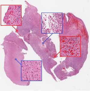
Two classification problem from WSI is selected by authors for evaluating their model. Those classification tasks are classifying gliomaand Non-Small-Cell Lung Carcinoma (NSCLC) cases into glioma and NSCLC subtypes which the typical resolution of a WSI in this dataset is 100K by 50K pixels. Both glioma and NSCLC are common cancers that lead cancer related death in different ages, and recognizing their subtype is a critical task that is essential for providing targeted therapies.

Patch Extraction and Segmentation

For training CNN, 1000 valid patches per image and per scale is extracted from WSIs which are non-overlapping given the WSI resolution. Each patch has the size of 500*500and for capturing the structures at different scales, patches are extracted from 20x (0.5 microns per pixel) and 5x (2.0 microns per pixel) objective magnifications. For avoiding overfitting, three kinds of data augmentation are employed in every iteration on a random 400×400 sub-patch from each 500×500 patch as: 1. Rotating randomly, 2. Mirroring the sub-patch and 3. Adjusting the amount of Hematoxylin and eosin stained on the tissue randomly. For doing the third one the RGB color of the tissue is decomposed into the [math]\displaystyle{ H }[/math]&[math]\displaystyle{ E }[/math] color space. Then, the magnitude of [math]\displaystyle{ H }[/math] and [math]\displaystyle{ E }[/math] of every pixel is multiplied by two i.i.d. Gaussian random variables with expectations equal to one.

CNN Architecture

Table 1: Architecture of the CNN used in glioma and NSCLC classification. ReLU+LRN is a sequence of Rectified Linear Units (ReLU) followed by Local Response Normalization (LRN). ReLU+Drop is a sequence of ReLU followed by dropout. The dropout probability is [math]\displaystyle{ 0.5 }[/math].

Table.1 shows the overall architecture of the CNN.
The CAFFE toolbox was utilized for its implementation and trained that on a single NVidia Tesla K40 GPU.

Experimental Set Up

A random 80% of the WSI bags were selected for the train, while 20% others left for test. Also, depending on the method, train data was subsequently divided into two parts: (i) train for the first-level model, which estimates hidden labels for instances in the bag, (ii) train for the second-level model which is responsible for decision fusion.

The authors of the paper present the performance of 14 algorithms, but we will discuss only 5 the most interesting ones:

1. CNN-LR: CNN followed by logistic regression as a second-level model to predict image labels. One tenth of the patches in each image is hidden for the CNN to train the logistic regression.
2. EM-CNN-LR: EM-based method with logistic regression as second-level model
3. EM-CNN-SVM: EM-based method with SVM as second-level model
4. EM-Finetune-CNN-LR: similar to EM-CNN-LR, but CNN wasn’t trained from scratch. Authors performed a fine-tuning of a pretrained 16-layer CNN model by training it on discriminative patches.
5. EM-Finetune-CNN-SVM: similar to Em-Finetune-CNN-LR, but with SVM as second-level model

Results

WSI of Glioma Classification

6 subtypes of glioma WSI have been tested in this paper: Glioblastoma (GBM), Oligodendroglioma (OD), Oligoastrocytoma (OA), Diffuse astrocytoma (DA), Anaplastic astrocytoma (AA), Anaplastic oligodendroglioma (AO). The latter 5 subtypes are collectively referred to as Low-Grade Glioma (LGG).

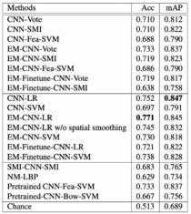
Table 2 on the left represents glioma classification results. The proposed EM-CNN-LR method achieved the best result, with an accuracy of 0.77, close to inter-observer agreement between pathologists, with an accuracy of 70%.

The comparison between GBM vs LGG yielded a 97% accuracy, with 51.3% chance.

In addition, the LGG-subtype classification resulted in a 57.1% accuracy with 36.7% chance.

The authors were the first to propose classifying 5 subtypes at once automatically, which is a lot more difficult to accomplish compared to the benchmark GBM vs LGG classification. Note that the OA subtype caused the most confusion because it is a mixed glioma.

WSI of NSCLC Classification

3 subtypes of Non-Small-Cell Lung Carcinoma (NSCLC) WSI have been tested in this paper: Squamous cell carcinoma (SCC), Adenocarcinoma (ADC), ADC with mixed subtypes (ADC-mix). Cohen’s kappa (κ) is used to measure inter-rater reliability.

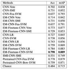
Table 3 on the left represents NSCLC classification results. The proposed EM-CNN-SVM and EM-Finetune-CNN-SVM methods achieved the best result, with an accuracy of 0.759 and 0.798, respectively, close to inter-observer agreement between pathologists.

For the comparison between SCC vs non-SCC, the inter-observer agreement between pulmonary pathology experts and between community pathologists are κ=0.64 and κ=0.41 respectively, and authors achieved κ=0.75. In addition, for the comparison between ADC vs non-ADC, the inter-observer agreement between pulmonary pathology experts and between community pathologists are κ=0.69 and κ=0.46 respectively, and authors achieved κ=0.60. We conclude that the results appear close to inter-observer agreement.

Note that ADC-mix was difficult to classify using the proposed methods as it contains visual features of multiple NSCLC subtypes.

Conclusion

Expectation-Maximization (EM) based method that identifies discriminative patches automatically has been proposed for patch-based Convolutional Neural Network (CNN) training. The algorithm was successful in classifying the various subtypes of cancer given Whole Slide Tissue Image (WSI) of patients with similar accuracy as pathologists. Note that performance of the patch-based CNN has been demonstrated to be more favorable to an image-based CNN.

References

[1] A. Cruz-Roa, A. Basavanhally, F. Gonzalez, H. Gilmore, M. Feldman, S. Ganesan, N. Shih, J. Tomaszewski, and A. Madabhushi. Automatic detection of invasive ductal carcinoma in whole slide images with convolutional neural networks. In Medical Imaging, 2014. 2, 3
[2] H. S. Mousavi, V. Monga, G. Rao, and A. U. Rao. Automated discrimination of lower and higher grade gliomas based on histopathological image analysis. JPI, 2015. 2, 6
[3] Y. Xu, Z. Jia, Y. Ai, F. Zhang, M. Lai, E. I. Chang, et al. Deep convolutional activation features for large scale brain tumor histopathology image classification and segmentation. In ICASSP, 2015. 2, 5, 6
[4] E. Cosatto, P.-F. Laquerre, C. Malon, H.-P. Graf, A. Saito, T. Kiyuna, A. Marugame, and K. Kamijo. Automated gastric cancer diagnosis on h&e-stained sections; ltraining a classifier on a large scale with multiple instance machine learning. In Medical Imaging, 2013. 2
[5] Y. Xu, T. Mo, Q. Feng, P. Zhong, M. Lai, E. I. Chang, et al. Deep learning of feature representation with multiple instance learning for medical image analysis. In ICASSP, 2014. 2
[6] J. Ramon and L. De Raedt. Multi instance neural networks. 2000. 2, 3
[7] Z.-H. Zhou and M.-L. Zhang. Neural networks for multiinstance learning. In ICIIT, 2002. 2, 3
[8] S. Poria, E. Cambria, and A. Gelbukh. Deep convolutional neural network textual features and multiple kernel learning for utterance-level multimodal sentiment analysis. 3
[9] A. Seff, L. Lu, K. M. Cherry, H. R. Roth, J. Liu, S. Wang, J. Hoffman, E. B. Turkbey, and R. M. Summers. 2d view aggregation for lymph node detection using a shallow hierarchy of linear classifiers. In MICCAI. 2014. 3, 4