One-Shot Object Detection with Co-Attention and Co-Excitation
Presented By
Gautam Bathla
Background
Object Detection is a technique where the model gets an image as an input and outputs the class and location of all the objects present in the image. The aim is to take a query image patch whose class label is not included in the training data and detect all instances of the same class in a target image.
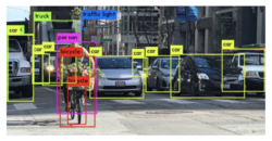
Figure 1 shows an example where the model identifies and locates all the instances of different objects present in the image successfully. It encloses each object within a bounding box and annotates each box with the class of the object present inside the box.
State-of-the-art object detectors are trained on thousands of images for different classes before the model can accurately predict the class and spatial location for unseen images belonging to the classes the model has been trained on. When a model is trained with K labeled instances for each of N classes, then this setting is known as N-way K-shot classification. K = 0 for zero-shot learning, K = 1 for one-shot learning and K > 1 for few-shot learning.
Introduction
This paper tackles the problem of one-shot object detection, where the model needs to find all the instances in the target image of the object in the query image for a given query image p. The target and query image do not need to be exactly the same and are allowed to have variations as long as they share some attributes so that they can belong to the same category. In this paper, the authors have made contributions to three technical areas. First is the use of non-local operations to generate better region proposals for the target image based on the query image. This operation can be thought of as a co-attention mechanism. The second contribution is proposing a Squeeze and Co-Excitation mechanism to identify and give more importance to relevant features to filter out relevant proposals and hence the instances in the target image. Third, the authors designed a margin-based ranking loss which will be useful for predicting the similarity of region proposals with the given query image irrespective of whether the label of the class is seen or unseen during the training process. This paper introduces squeeze and co-excitation to extract the feature of classification object and proved that this architecture performs well to do object detection in both seen and never-seen classes.
Previous Work
All state-of-the-art object detectors are variants of deep convolutional neural networks. There are two types of object detectors:
1) Two-Stage Object Detectors: These types of detectors generate region proposals in the first stage whereas classify and refine the proposals in the second stage. Eg. FasterRCNN [1].
2) One Stage Object Detectors: These types of detectors directly predict bounding boxes and their corresponding labels based on a fixed set of anchors. Eg. CornerNet [2].
The work done to tackle the problem of few-shot object detection is based on transfer learning [3], meta-learning [4], and metric-learning.
1) Transfer Learning: Chen et al. [3] proposed a regularization technique to reduce overfitting when the model is trained on just a few instances for each class belonging to unseen classes.
2) Meta-Learning: Kang et al. [4] trained a meta-model to re-weight the learned weights of an image extracted from the base model.
3) Metric-Learning: These frameworks replace the conventional classifier layer with the metric-based classifier layer.
Approach
Let [math]\displaystyle{ C }[/math] be the set of classes for this object detection task. Since one-shot object detection task needs unseen classes during inference time, therefore we divide the set of classes into two categories as follows:
where [math]\displaystyle{ C_0 }[/math] represents the classes that the model is trained on and [math]\displaystyle{ C_1 }[/math] represents the classes on which the inference is done.

Figure 2 shows the architecture of the model proposed in this paper. The model architecture is based on FasterRCNN [1], and ResNet-50 [5] has been used as the backbone for extracting features from the images. The target image and the query image are first passed through the ResNet-50 module to extract the features from the same convolutional layer. The features obtained are next passed into the Non-local block as input and the output consists of weighted features for each of the images. The new weighted feature set for both images is passed through Squeeze and Co-excitation block which outputs the re-weighted features which act as an input to the Region Proposal Network (RPN) module. RCNN module also consists of a new loss that is designed by the authors to rank proposals in order of their relevance.
Non-Local Object Proposals
The need for non-local object proposals arises because the RPN module used in Faster R-CNN [1] has access to bounding box information for each class in the training dataset. The dataset used for training and inference in the case of Faster R-CNN [1] is not exclusive. In this problem, as we have defined above that we divide the dataset into two parts, one part is used for training and the other is used during inference. Therefore, the classes in the two sets are exclusive. If the conventional RPN module is used, then the module will not be able to generate good proposals for images during inference because it will not have any information about the presence of bounding-box for those classes.
To resolve this problem, a non-local operation is applied to both sets of features. This non-local operation is defined as: \begin{align} y_i = \frac{1}{C(z)} \sum_{\forall j}^{} f(x_i, z_j)g(z_j) \tag{1} \label{eq:op} \end{align}
where x is a vector on which this operation is applied, z is a vector which is taken as an input reference, i is the index of output position, j is the index that enumerates over all possible positions, C(z) is a normalization factor, [math]\displaystyle{ f(x_i, z_j) }[/math] is a pairwise function like Gaussian, Dot product, concatenation, etc., [math]\displaystyle{ g(z_j) }[/math] is a linear function of the form [math]\displaystyle{ W_z \times z_j }[/math], and y is the output of this operation.
Let the feature maps obtained from the ResNet-50 model be [math]\displaystyle{ \phi{(I)} \in R^{N \times W_I \times H_I} }[/math] for target image I and [math]\displaystyle{ \phi{(p)} \in R^{N \times W_p \times H_p} }[/math] for query image p. Taking [math]\displaystyle{ \phi{(p)} }[/math] as the input reference, the non-local operation is applied to [math]\displaystyle{ \phi{(I)} }[/math] and results in a non-local block, [math]\displaystyle{ \psi{(I;p)} \in R^{N \times W_I \times H_I} }[/math] . Analogously, we can derive the non-local block [math]\displaystyle{ \psi{(p;I)} \in R^{N \times W_p \times H_p} }[/math] using [math]\displaystyle{ \phi{(I)} }[/math] as the input reference.
We can express the extended feature maps as:
\begin{align} {F(I) = \phi{(I)} \oplus \psi{(I;p)} \in R^{N \times W_I \times H_I}} \ \ ;\ \ {F(p) = \phi{(p)} \oplus \psi{(p;I)} \in R^{N \times W_p \times H_p}} \tag{2} \label{eq:o1} \end{align}
where F(I) denotes the extended feature map for target image I, F(p) denotes the extended feature map for query image p and [math]\displaystyle{ \oplus }[/math] denotes element-wise sum over the feature maps [math]\displaystyle{ \phi{} }[/math] and [math]\displaystyle{ \psi{} }[/math].
As can be seen above, the extended feature set for the target image I do not only contain features from I but also the weighted sum of the target image and the query image. The same can be observed for the query image. This weighted sum is a co-attention mechanism and with the help of extended feature maps, better proposals are generated when inputted to the RPN module.
Squeeze and Co-Excitation
The two feature maps generated from the non-local block above can be further related by identifying the important channels and therefore, re-weighting the weights of the channels. This is the basic purpose of this module. The Squeeze layer summarizes each feature map by applying Global Average Pooling (GAP) on the extended feature map for the query image. The Co-Excitation layer gives attention to feature channels that are important for evaluating the similarity metric. The whole block can be represented as:
\begin{align} SCE(F(I), F(p)) = w \ \ ;\ \ F(\tilde{p}) = w \odot F(p) \ \ ;\ \ F(\tilde{I}) = w \odot F(I)\tag{3} \label{eq:op2} \end{align}
where w is the excitation vector, [math]\displaystyle{ F(\tilde{p}) }[/math] and [math]\displaystyle{ F(\tilde{I}) }[/math] are the re-weighted features maps for query and target image respectively.
In between the Squeeze layer and Co-Excitation layer, there exist two fully-connected layers followed by a sigmoid layer which helps to learn the excitation vector w. The Channel Attention module in the architecture is basically these fully-connected layers followed by a sigmoid layer.
Margin-based Ranking Loss
The authors have defined a two-layer MLP network ending with a softmax layer to learn a similarity metric which will help rank the proposals generated by the RPN module. In the first stage of training, each proposal is annotated with 0 or 1 based on the IoU value of the proposal with the ground-truth bounding box. If the IoU value is greater than 0.5 then that proposal is labeled as 1 (foreground) and 0 (background) otherwise.
Let q be the feature vector obtained after applying GAP to the query image patch obtained from the Squeeze and Co-Excitation block and r be the feature vector obtained after applying GAP to the region proposals generated by the RPN module. The two vectors are concatenated to form a new vector x which is the input to the two-layer MLP network designed. We can define x = [[math]\displaystyle{ r^T;q^T }[/math]]. Let M be the model representing the two-layer MLP network, then [math]\displaystyle{ s_i = M(x_i) }[/math], where [math]\displaystyle{ s_i }[/math] is the probability of [math]\displaystyle{ i^{th} }[/math] proposal being a foreground proposal based on the query image patch q.
The margin-based ranking loss is given by:
\begin{align} L_{MR}(\{x_i\}) = \sum_{i=1}^{K}y_i \times max\{m^+ - s_i, 0\} + (1-y_i) \times max\{s_i - m^-, 0\} + \delta_{i} \tag{4} \label{eq:op3} \end{align} \begin{align} \delta_{i} = \sum_{j=i+1}^{K}[y_i = y_j] \times max\{|s_i - s_j| - m^-, 0\} + [y_i \ne y_j] \times max\{m^+ - |s_i - s_j|, 0\} \tag{5} \label{eq:op4} \end{align}
where [.] is the Iversion bracket, i.e. the output will be 1 if the condition inside the bracket is true and 0 otherwise, [math]\displaystyle{ m^+ }[/math] is the expected lower bound probability for predicting a foreground proposal, [math]\displaystyle{ m^- }[/math] is the expected upper bound probability for predicting a background proposal and [math]\displaystyle{ K }[/math] is the number of candidate proposals from RPN.
The total loss for the model is given as:
\begin{align} L = L_{CE} + L_{Reg} + \lambda \times L_{MR} \tag{6} \label{eq:op5} \end{align}
where [math]\displaystyle{ L_{CE} }[/math] is the cross-entropy loss, [math]\displaystyle{ L_{Reg} }[/math] is the regression loss for bounding boxes of Faster R-CNN [1] and [math]\displaystyle{ L_{MR} }[/math] is the margin-based ranking loss defined above.
For this paper, [math]\displaystyle{ m^+ }[/math] = 0.7, [math]\displaystyle{ m^- }[/math] = 0.3, [math]\displaystyle{ \lambda }[/math] = 3, K = 128, C(z) in \eqref{eq:op} is the total number of elements in a single feature map of vector z, and [math]\displaystyle{ f(x_i, z_j) }[/math] in \eqref{eq:op} is a dot product operation. \begin{align} f(x_i, z_j) = \alpha(x_i)^T \beta(z_j)\ \ ;\ \ \alpha(x_i) = W_{\alpha} x_i \ \ ;\ \ \beta(z_j) = W_{\beta} z_j \tag{7} \label{eq:op6} \end{align}
Results
The model is trained and tested on two popular datasets, VOC and COCO. The ResNet-50 model was pre-trained on a reduced dataset by removing all the classes present in the COCO dataset, thus ensuring that the model has not seen any of the classes belonging to the inference images.
Results on VOC Dataset

For the VOC dataset, the model is trained on the union of VOC 2007 train and validation sets and VOC 2012 train and validation sets, whereas the model is tested on VOC 2007 test set. From the VOC results (Table 1), it can be seen that the model with pre-trained ResNet-50 on a reduced training set as the CNN backbone (Ours(725)) achieves better performance on seen and unseen classes than the baseline models. When the pre-trained ResNet-50 on the full training set (Ours(1K)) is used as the CNN backbone, then the performance of the model is increased significantly.
Results on MSCOCO Dataset


The model is trained on the COCO train2017 set and evaluated on the COCO val2017 set. The classes are divided into four groups and the model is trained with images belonging to three splits, whereas the evaluation is done on the images belonging to the fourth split. From Table 2, it is visible that the model achieved better accuracy than the baseline model. The bar chart value in the split figure shows the performance of the model on each class separately. The model is having some difficulties when predicting images belonging to classes like the book (split2), handbag (split3), and tie (split4) because of variations in their shape and textures.
Overall Performance
For VOC, the model that uses the reduced ImageNet model backbone with 725 classes achieves a better performance on both the seen and unseen classes. Remarkable improvements in the performance are seen with the backbone with 1000 classes. For COCO, the model achieves better accuracy than the Siamese Mask-RCNN model for both the seen and unseen classes.
Ablation Studies
Effect of all the proposed techniques on the final result

Figure 3 shows the effect of the three proposed techniques on the evaluation metric. The model performs worst when neither Co-attention nor Co-excitation mechanism is used. But, when either Co-attention or Co-excitation is used then the performance of the model is improved significantly. The model performs best when all the three proposed techniques are used.
In order to understand the effect of the proposed modules, the authors analyzed each module separately.
Visualizing the effect of Non-local RPN
To demonstrate the effect of Non-local RPN, a heatmap of generated proposals is constructed. Each pixel is assigned the count of how many proposals cover that particular pixel and the counts are then normalized to generate a probability map.
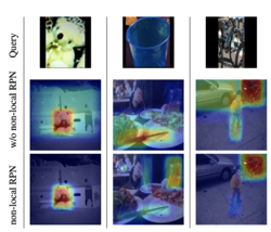
From Figure 4, it can be seen that when a non-local RPN is used instead of a conventional RPN, the model is able to give more attention to the relevant region in the target image.
Analyzing and Visualizing the effect of Co-Excitation
To visualize the effect of excitation vector w, the vector is calculated for all images in the inference set which are then averaged over images belonging to the same class, and a pair-wise Euclidean distance between classes is calculated.
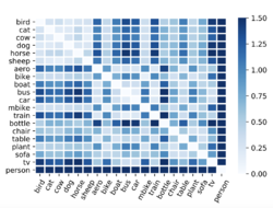
From Figure 5, it can be observed that the Co-Excitation mechanism is able to assign meaningful weight distribution to each class. The weights for classes related to animals are closer to each other and the person class is not close to any other class because of the absence of common attributes between person and any other class in the dataset.
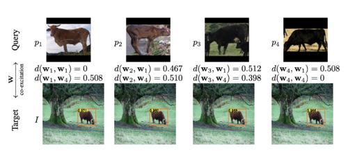
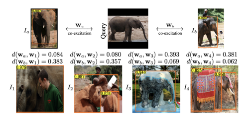
To analyze the effect of Co-Excitation, the authors used two different scenarios. In the first scenario (Figure 6, left), the same target image is used for different query images. [math]\displaystyle{ p_1 }[/math] and [math]\displaystyle{ p_2 }[/math] query images have a similar color as the target image whereas [math]\displaystyle{ p_3 }[/math] and [math]\displaystyle{ p_4 }[/math] query images have a different color object as compared to the target image. When the pair-wise Euclidean distance between the excitation vector in the four cases was calculated, it can be seen that [math]\displaystyle{ w_2 }[/math] was closer to [math]\displaystyle{ w_1 }[/math] as compared to [math]\displaystyle{ w_4 }[/math] and [math]\displaystyle{ w_3 }[/math] was closer to [math]\displaystyle{ w_4 }[/math] as compared to [math]\displaystyle{ w_1 }[/math]. Therefore, it can be concluded that [math]\displaystyle{ w_1 }[/math] and [math]\displaystyle{ w_2 }[/math] give more importance to the texture of the object whereas [math]\displaystyle{ w_3 }[/math] and [math]\displaystyle{ w_4 }[/math] give more importance to channels representing the shape of the object.
The same observation can be analyzed in scenario 2 (Figure 6, right) where the same query image was used for different target images. [math]\displaystyle{ w_1 }[/math] and [math]\displaystyle{ w_2 }[/math] are closer to [math]\displaystyle{ w_a }[/math] than [math]\displaystyle{ w_b }[/math] whereas [math]\displaystyle{ w_3 }[/math] and [math]\displaystyle{ w_4 }[/math] are closer to [math]\displaystyle{ w_b }[/math] than [math]\displaystyle{ w_a }[/math]. Since images [math]\displaystyle{ I_1 }[/math] and [math]\displaystyle{ I_2 }[/math] have a similar color object as the query image, we can say that [math]\displaystyle{ w_1 }[/math] and [math]\displaystyle{ w_2 }[/math] give more weightage to the channels representing the texture of the object, and [math]\displaystyle{ w_3 }[/math] and [math]\displaystyle{ w_4 }[/math] give more weightage to the channels representing shape.
Conclusion
The resulting one-shot object detector outperforms all the baseline models on VOC and COCO datasets. The authors have also provided insights about how the non-local proposals, serving as a co-attention mechanism, can generate relevant region proposals in the target image and put emphasis on the important features shared by both target and query image.
Related Work
Object detection SOTA object detectors are mostly deep convolutional neural networks. A popular pipeline is a two-stage approach, where detectors first generate a set of region proposals and then classify the proposals. The latest version is called Faster R-CNN [6], which works by replacing the grouping-based proposals originally found in R-CNN with a regional proposal network.
Few-shot classification via metric learning The aim of this is to derive a similarity metric that can be used to infer unseen classes. One approach is to use Siamese networks, which learn a general similarity metric from using paired training data to decide whether the pair belongs to the same class. Then, during inference, the network matches unlabelled observations with a one-shot support set, where classification is done by asking which observed class is most similar [7].
Few-shot object detection The problem of detection, like classification, can be assessed in a few-shot setting. However, the problem is quite novel so only preliminary results from transfer learning, meta learning, and metric learning exist.
Critiques
The techniques proposed by the authors improve the performance of the model significantly as we saw that when either of Co-attention or Co-excitation is used along with Margin-based ranking loss then the model can detect the instances of query object in the target image. Also, the model trained is generic and does not require any training/fine-tuning to detect any unseen classes in the target image. The loss metric designed makes the learning process not to rely on only the labels of images since the proposed metric annotates each proposal as a foreground or a background which is then used to calculate the metric. Since it is exploiting many deep neural networks inside the main architecture, one critique that comes across is how time-consuming the proposed model is. The paper could have elucidated it more thoroughly whether the method is too time-consuming or not.
Source Code
link One-Shot-Object-Detection
References
[1] Shaoqing Ren, Kaiming He, Ross B. Girshick, and Jian Sun. Faster R-CNN: towards real-time object detection with region proposal networks. In Advances in Neural Information Processing Systems 28: Annual Conference on Neural Information Processing Systems 2015, December 7-12, 2015, Montreal, Quebec, Canada, pages 91–99, 2015.
[2] Hei Law and Jia Deng. Cornernet: Detecting objects as paired keypoints. In Computer Vision - ECCV 2018 - 15th European Conference, Munich, Germany, September 8-14, 2018, Proceedings, Part XIV, pages 765–781, 2018
[3] Hao Chen, Yali Wang, Guoyou Wang, and Yu Qiao. LSTD: A low-shot transfer detector for object detection. In Proceedings of the Thirty-Second AAAI Conference on Artificial Intelligence, (AAAI-18), the 30th innovative Applications of Artificial Intelligence (IAAI-18), and the 8th AAAI Symposium on Educational Advances in Artificial Intelligence (EAAI-18), New Orleans, Louisiana, USA, February 2-7, 2018, pages 2836–2843, 2018.
[4] Bingyi Kang, Zhuang Liu, Xin Wang, Fisher Yu, Jiashi Feng, and Trevor Darrell. Few-shot object detection via feature reweighting. CoRR, abs/1812.01866, 2018.
[5] K. He, X. Zhang, S. Ren and J. Sun, "Deep Residual Learning for Image Recognition," 2016 IEEE Conference on Computer Vision and Pattern Recognition (CVPR), Las Vegas, NV, 2016, pp. 770-778, doi: 10.1109/CVPR.2016.90.
[6] Shaoqing Ren, Kaiming He, Ross B. Girshick, and Jian Sun. Faster R-CNN: towards real-time object detection with region proposal networks. In Advances in Neural Information Processing Systems 28: Annual Conference on Neural Information Processing Systems 2015, December 7-12, 2015, Montreal, Quebec, Canada, pages 91–99, 2015.
[7] Gregory R. Koch. Siamese neural networks for one-shot image recognition. 2015.