Model-Agnostic Meta-Learning for Fast Adaptation of Deep Networks

Introduction & Background

Learning quickly is a hallmark of human intelligence, whether it involves recognizing objects from a few examples or quickly learning new skills after just minutes of experience. Meta-learning is a subfield of machine learning where automatic learning algorithms are applied on meta-data about machine learning experiments. The goal of meta-learning is to train a model on a variety of learning tasks, such that it can solve new learning tasks using only a small number of training samples. In this work, we propose a meta-learning algorithm that is general and model-agnostic, in the sense that it can be directly applied to any learning problem and model that is trained with a gradient descent procedure. Our focus is on deep neural network models, but we illustrate how our approach can easily handle different architectures and different problem settings, including classification, regression, and policy gradient reinforcement learning, with minimal modification. Unlike prior meta-learning methods that learn an update function or learning rule [1,2,3,4], this algorithm does not expand the number of learned parameters nor place constraints on the model architecture (e.g. by requiring a recurrent model [5] or a Siamese network [6]), and it can be readily combined with fully connected, convolutional, or recurrent neural networks. It can also be used with a variety of loss functions, including differentiable supervised losses and nondifferentiable reinforcement learning objectives.

The primary contribution of this work is a simple model and task-agnostic algorithm for meta-learning that trains a model’s parameters such that a small number of gradient updates will lead to fast learning on a new task. The paper shows the effectiveness of the proposed algorithm in different domains, including classification, regression, and reinforcement learning problems.

Key Idea

Arguably, the biggest success story of transfer learning has been initializing vision network weights using pre-trained ImageNet. In particular, when approaching any new vision task, the well-known paradigm is to first collect labeled data for the task, acquire a network pre-trained on ImageNet classification, and then fine-tune the network on the collected data using gradient descent. Using this approach, neural networks can more effectively learn new image-based tasks from modestly-sized datasets. However, pre-training does not go very far, because, the last layers of the network still need to be heavily adapted to the new task, datasets that are too small, as in the few-shot setting, will still cause severe overfitting. Furthermore, we unfortunately don’t have an analogous pre-training scheme for non-vision domains such as speech, language, and control.

What if we directly optimized for an initial representation that can be effectively fine-tuned from a small number of examples? This is exactly the idea behind this paper, model-agnostic meta-learning (MAML). Like other meta-learning methods, MAML trains over a wide range of tasks. It trains for a representation that can be quickly adapted to a new task, via a few gradient steps. The meta-learner seeks to find an initialization that is not only useful for adapting to various problems but also can be adapted quickly (in a small number of steps) and efficiently (using only a few examples).

The key idea underlying this method is to train the model’s initial parameters such that the model has maximal performance on a new task after the parameters have been updated through one or more gradient steps computed with a small amount of data from that new task. This can be viewed from a feature learning standpoint as building an internal representation that is broadly suitable for many tasks. If the internal representation is suitable for many tasks, simply fine-tuning the parameters slightly (e.g. by primarily modifying the top layer weights in a feedforward model) can produce good results.

Model-Agnostic Meta Learning (MAML)

The goal of the proposed model is the rapid adaptation, which means learning a new function from only a few input/output pairs for that task, using prior data from similar tasks for meta-learning. This setting is usually formalized as few-shot learning.

Problem set-up

The goal of few-shot meta-learning is to train a model that can quickly adapt to a new task using only a few data points and training iterations. To do so, the model is trained during a meta-learning phase on a set of tasks, such that it can then be adapted to a new task using only a small number of parameter updates. In effect, the meta-learning problem treats entire tasks as training examples.

Let us consider a model denoted by $f$, that maps the observation $\mathbf{x}$ into the output variable $a$. During meta-learning, the model is trained to be able to adapt to a large or infinite number of tasks.

Let us consider a generic notion of task as below. Each task $\mathcal{T} = \{\mathcal{L}(\mathbf{x}_1,a_1,\mathbf{x}_2,a_2,..., \mathbf{x}_H,a_H), q(\mathbf{x}_1),q(\mathbf{x}_{t+1}|\mathbf{x}_t,a_t),H \}$, consists of a loss function $\mathcal{L}$, a distribution over initial observations $q(\mathbf{x}_1)$, a transition distribution $q(\mathbf{x}_{t+1}|\mathbf{x}_t)$, and an episode length $H$. In i.i.d. supervised learning problems, the length $H =1$. The model may generate samples of length $H$ by choosing an output at at each time $t$. The cost $\mathcal{L}$ provides a task-specific feedback, which is defined based on the nature of the problem.

A distribution over tasks is denoted by $p(\mathcal{T})$. In the K-shot learning setting, the model is trained to learn a new task $\mathcal{T}_i$ drawn from $p(\mathcal{T})$ from only K samples drawn from $q_i$ and feedback $\mathcal{L}_{\mathcal{T}_i}$ generated by $\mathcal{T}_i$. During meta-training, a task $\mathcal{T}_i$ is sampled from $p(\mathcal{T})$, the model is trained with K samples and feedback from the corresponding loss $\mathcal{L}(\mathcal{T}_i)$ from $\mathcal{T}_i$, and then tested on new samples from $T_i$. The model $f$ is then improved by considering how the test error on new data from $q_i$ changes with respect to the parameters. In effect, the test error on sampled tasks $\mathcal{T}_i$ serves as the training error of the meta-learning process. At the end of meta-training, new tasks are sampled from $p(\mathcal{T})$, and meta-performance is measured by the model’s performance after learning from K samples. Notice that tasks used for meta-testing are held out during meta-training.

MAML Algorithm

Figure 1: Diagram of the MAML algorithm

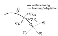
The paper proposes a method that can learn the parameters of any standard model via meta-learning in such a way as to prepare that model for fast adaptation. The intuition behind this approach is that some internal representations are more transferable than others. Since the model will be fine-tuned using a gradient-based learning rule on a new task, we will aim to learn a model in such a way that this gradient-based learning rule can make rapid progress on new tasks drawn from $p(\mathcal{T})$, without overfitting. In effect, we will aim to find model parameters that are sensitive to changes in the task, such that small changes in the parameters will produce large improvements on the loss function of any task drawn from $p(\mathcal{T})$. Fig. 1 is a visualization of MMAML algorithm – suppose we are seeking to find a set of parameters $\theta$ that are highly adaptable. During the course of meta-learning (the bold line), MAML optimizes for a set of parameters such that when a gradient step is taken with respect to a particular task $i$ (the gray lines), the parameters are close to the optimal parameters $θ^∗_i$ for task $i$.

Note that there is no assumption about the form of the model. The only assumption is that it is parameterized by a vector of parameters $\theta$, and the loss is smooth so that the parameters can be leaned using gradient-based techniques. Formally let us assume that the model is denoted by $f_{\theta}$. When adapting to a new task $\mathcal{T}_i $, the model’s parameters $\theta$ become $\theta_i'$. In our method, the updated parameter vector $\theta_i'$ is computed using one or more gradient descent updates on task $\mathcal{T}_i $. For example, when using one gradient update:

$$ \theta_i ' = \theta - \alpha \nabla_{\theta }\mathcal{L}_{\mathcal{T}_i}(f_{\theta}). $$

Here $\alpha$ is the learning rate (or the step size) of each task and considered as a hyperparameter. They consider a single step of an update for the rest of the paper, for the sake of the simplicity.

The model parameters are trained by optimizing for the performance of $f_{\theta_i'}$ with respect to $\theta$ across tasks sampled from $p(\mathcal{T})$. More concretely, the meta-objective is as follows:

$$ \min_{\theta} \sum \limits_{\mathcal{T}_i \sim p(\mathcal{T})} \mathcal{L}_{\mathcal{T}_i} (f_{\theta_i'}) = \sum \limits_{\mathcal{T}_i \sim p(\mathcal{T})} \mathcal{L}_{\mathcal{T}_i} (f_{\theta - \alpha \nabla_{\theta }\mathcal{L}_{\mathcal{T}_i}(f_{\theta})}) $$

Note that the meta-optimization is performed over the model parameters $\theta$, whereas the objective is computed using the updated model parameters $\theta'$. The model aims to optimize the model parameters such that one or a small number of gradient step on a new task will produce maximally effective behavior on that task.

Therefore the meta-learning across the tasks is performed via stochastic gradient descent (SGD), such that the model parameters $\theta$ are updated as:

$$ \theta \gets \theta - \beta \nabla_{\theta } \sum \limits_{\mathcal{T}_i \sim p(\mathcal{T})} \mathcal{L}_{\mathcal{T}_i} (f_{\theta_i'}) $$ where $\beta$ is the meta step size. Outline of the algorithm is shown in Algorithm 1.

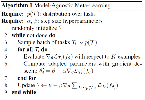
The MAML meta-gradient update involves a gradient through a gradient. Computationally, this requires an additional backward pass through f to compute Hessian-vector products, which is supported by standard deep learning libraries such as TensorFlow.

Different Types of MAML

In this section, the MAML algorithm is discussed for different supervised learning and reinforcement learning tasks. The differences between each of these tasks are in their loss function and the way the data is generated. In general, this method does not require additional model parameters nor using any additional meta-learner to learn the update of parameters. Compared to other approaches that tend to “learn to compare new examples in a learned metric space using e.g. Siamese networks or recurrence with attention mechanisms”, the proposed method can be generalized to any other problems including classification, regression and reinforcement learning.

Supervised Regression and Classification

Few-shot learning is well-studied in this field. For these two types of tasks, the horizon $H$ is equal to 1, since the model accepts a single input and produces a single output, rather than a sequence of inputs and outputs. The task ${\mathcal{T}_i}$ generates $K$ i.i.d. observations $x$ from $q_i$, and the task loss is represented by the error between the model’s output for x and the corresponding target values y for that observation and task

Although any common classification and regression objectives can be used as the loss, the paper uses the following losses for these two tasks.

Regression : For regression we use the mean-square error (MSE):

$$ \mathcal{L}_{\mathcal{T}_i} (f_{\theta}) = \sum \limits_{\mathbf{x}^{(j)}, \mathcal{y}^{(j)} \sim \mathcal{T}_i} \parallel f_{\theta} (\mathbf{x}^{(j)}) - \mathbf{y}^{(j)}\parallel_2^2 $$

where $\mathbf{x}^{(j)}$ and $\mathbf{y}^{(j)}$ are the input/output pair sampled from task $\mathcal{T}_i$. In K-shot regression tasks, K input/output pairs are provided for learning for each task.

Classification: For classification we use the cross entropy loss:

$$ \mathcal{L}_{\mathcal{T}_i} (f_{\theta}) = \sum \limits_{\mathbf{x}^{(j)}, \mathcal{y}^{(j)} \sim \mathcal{T}_i} \mathbf{y}^{(j)} \log f_{\theta}(\mathbf{x}^{(j)}) + (1-\mathbf{y}^{(j)}) \log (1-f_{\theta}(\mathbf{x}^{(j)})) $$

According to the conventional terminology, K-shot classification tasks use K input/output pairs from each class, for a total of $NK$ data points for N-way classification.

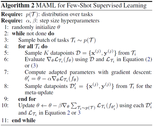
Given a distribution over tasks, these loss functions can be directly inserted into the equations in the previous section to perform meta-learning, as detailed in Algorithm 2.

Reinforcement Learning

In reinforcement learning (RL), the goal of few-shot meta learning is to enable an agent to quickly acquire a policy for a new test task using only a small amount of experience in the test setting. A new task might involve achieving a new goal or succeeding on a previously trained goal in a new environment. For example, an agent may learn how to navigate mazes very quickly so that, when faced with a new maze, it can determine how to reliably reach the exit with only a few samples.

Each RL task $\mathcal{T}_i$ contains an initial state distribution $q_i(\mathbf{x}_1)$ and a transition distribution $q_i(\mathbf{x}_{t+1}|\mathbf{x}_t,a_t)$ , and the loss $\mathcal{L}_{\mathcal{T}_i}$ corresponds to the (negative) reward function $R$. The entire task is therefore a Markov decision process (MDP) with horizon H, where the learner is allowed to query a limited number of sample trajectories for few-shot learning. Any aspect of the MDP may change across tasks in $p(\mathcal{T})$. The model being learned, $f_{\theta}$, is a policy that maps from states $\mathbf{x}_t$ to a distribution over actions $a_t$ at each timestep $t \in \{1,...,H\}$. The loss for task $\mathcal{T}_i$ and model $f_{\theta}$ takes the form

$$ \mathcal{L}_{\mathcal{T}_i}(f_{\theta}) = -\mathbb{E}_{\mathbf{x}_t,a_t \sim f_{\theta},q_{\mathcal{T}_i}} \big [\sum_{t=1}^H R_i(\mathbf{x}_t,a_t)\big ] $$

In K-shot reinforcement learning, K rollouts from $f_{\theta}$ and task $\mathcal{T}_i$, $(\mathbf{x}_1,a_1,...,\mathbf{x}_H)$, and the corresponding rewards $ R(\mathbf{x}_t,a_t)$, may be used for adaptation on a new task $\mathcal{T}_i$.

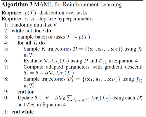
Since the expected reward is generally not differentiable due to unknown dynamics, we use policy gradient methods to estimate the gradient both for the model gradient update(s) and the meta-optimization. Since policy gradients are an on-policy algorithm, each additional gradient step during the adaptation of $f_{\theta}$ requires new samples from the current policy $f_{\theta_i}$ . We detail the algorithm in Algorithm 3, which has the same structure as Algorithm 2 but also which requires sampling trajectories from the environment corresponding to task $\mathcal{T}_i$ in steps 5 and 8. Here, a variety of improvements for policy gradient algorithm, including state or action-dependent baselines may also be used.

Experiments

Regression

We start with a simple regression problem that illustrates the basic principles of MAML. Each task involves regressing from the input to the output of a sine wave, where the amplitude and phase of the sinusoid are varied between tasks. Thus, $p(\mathcal{T})$ is continuous, and the input and output both have a dimensionality of 1. During training and testing, datapoints are sampled uniformly. The loss is the mean-squared error between the prediction and true value. The regressor is a neural network model with 2 hidden layers of size 40 with ReLU nonlinearities. When training with MAML, we use one gradient update with K = 10 examples with a fixed step size 0.01, and use Adam as the metaoptimizer [7]. The baselines are likewise trained with Adam. To evaluate performance, we fine-tune a single meta-learned model on varying numbers of K examples, and compare performance to two baselines: (a) pre-training on all of the tasks, which entails training a network to regress to random sinusoid functions and then, at test-time, fine-tuning with gradient descent on the K provided points, using an automatically tuned step size, and (b) an oracle which receives the true amplitude and phase as input.

We evaluate performance by fine-tuning the model learned by MAML and the pre-trained model on $K = \{ 5,10,20 \}$ datapoints. During fine-tuning, each gradient step is computed using the same $K$ datapoints. Results are shown in Fig 2.

Figure 2: Few-shot adaptation for the simple regression task. Left: Note that MAML is able to estimate parts of the curve where there are no datapoints, indicating that the model has learned about the periodic structure of sine waves. Right: Fine-tuning of a model pre-trained on the same distribution of tasks without MAML, with a tuned step size. Due to the often contradictory outputs on the pre-training tasks, this model is unable to recover a suitable representation and fails to extrapolate from the small number of test-time samples.

Classification

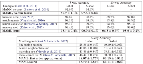
For classification evaluation, Omniglot and MiniImagenet datasets are used. The Omniglot dataset consists of 20 instances of 1623 characters from 50 different alphabets.

The experiment involves fast learning of N-way classification with 1 or 5 shots. The problem of N-way classification is set up as follows: select N unseen classes, provide the model with K different instances of each of the N classes and evaluate the model’s ability to classify new instances within the N classes. For Omniglot, 1200 characters are selected randomly for training, irrespective of the alphabet, and use the remaining for testing. The Omniglot dataset is augmented with rotations by multiples of 90 degrees.

The model follows the same architecture as the embedding function that has 4 modules with a 3-by-3 convolution and 64 filters, followed by batch normalization, a ReLU nonlinearity, and 2-by-2 max-pooling. The Omniglot images are downsampled to 28-by-28, so the dimensionality of the last hidden layer is 64. The last layer is fed into a softmax. For Omniglot, strided convolutions are used instead of max-pooling. For MiniImagenet, 32 filters per layer are used to reduce overfitting. In order to also provide a fair comparison against memory-augmented neural networks [7] and to test the flexibility of MAML, the results for a non-convolutional network are also provided.

Table 1: Few-shot classification on held-out Omniglot characters (top) and the MiniImagenet test set (bottom). MAML achieves results that are comparable to or outperform state-of-the-art convolutional and recurrent models. Siamese nets, matching nets, and the memory module approaches are all specific to classification and are not directly applicable to regression or RL scenarios. The $\pm$ shows 95% confidence intervals over tasks.

Reinforcement Learning

Several simulated continuous control environments are used for RL evaluation. In all of the domain, the MAML model is a neural network policy with two hidden layers of size 100, and ReLU activations. The gradient updates are computed using vanilla policy gradient and trust-region policy optimization (TRPO) is used as the meta-optimizer.

In order to avoid computing third derivatives, finite differences are computed to compute the Hessian-vector products for TRPO. For both learning and meta-learning updates, we use the standard linear feature baseline proposed by [8], which is fitted separately at each iteration for each sampled task in the batch.

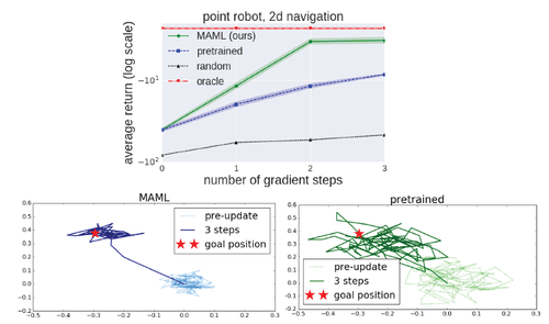
Three baseline models for the comparison are: (a) pretraining one policy on all of the tasks and then fine-tuning (b) training a policy from randomly initialized weights (c) an oracle policy which receives the parameters of the task as input, which for the tasks below corresponds to a goal position, goal direction, or goal velocity for the agent.

The baseline models of (a) and (b) are fine-tuned with gradient descent with a manually tuned step size.

2D Navigation: In the first meta-RL experiment, the authors study a set of tasks where a point agent must move to different goal positions in 2D, randomly chosen for each task within a unit square. The observation is the current 2D position, and actions correspond to velocity commands clipped to be in the range [-0.1; 0.1]. The reward is the negative squared distance to the goal, and episodes terminate when the agent is within 0:01 of the goal or at the horizon ofH = 100. The policy was trained with MAML to maximize performance after 1 policy gradient update using 20 trajectories. They compare the adaptation to a new task with up to 4 gradient updates, each with 40 samples. Results are shown in Fig. 3.

Figure 3: Top: quantitative results from 2D navigation task, Bottom: qualitative comparison between model learned with MAML and with fine-tuning from a pre-trained network

Locomotion. To study how well MAML can scale to more complex deep RL problems, we also study adaptation on high-dimensional locomotion tasks with the MuJoCo simulator [9]. The tasks require two simulated robots – a planar cheetah and a 3D quadruped (the “ant”) – to run in a particular direction or at a particular velocity. In the goal velocity experiments, the reward is the negative absolute value between the current velocity of the agent and a goal, which is chosen uniformly at random between 0 and 2 for the cheetah and between 0 and 3 for the ant. In the goal direction experiments, the reward is the magnitude of the velocity in either the forward or backward direction, chosen at random for each task in p(T ). The horizon is H = 200, with 20 rollouts per gradient step for all problems except the ant forward/backward task, which used 40 rollouts per step. The results in Figure 5 show that MAML learns a model that can quickly adapt its velocity and direction with even just a single gradient update, and continues to improve with more gradient steps. The results also show that, on these challenging tasks, the MAML initialization substantially outperforms random initialization and pretraining.

Figure 4: Reinforcement learning results for the half-cheetah and ant locomotion tasks, with the tasks shown on the far right.

A conceptual method to achieve fast adaptation in language modeling tasks ( not been experimented on by the authors) would be to explore methods of attaching an Attention Kernel which results in a simple and differentiable loss. It has been implemented in One-Shot Language Modeling along with state-of-the-art improvements in one-shot learning on Imagenet and Omniglot [11].

Conclusion

The paper introduced a meta-learning method based on learning easily adaptable model parameters through gradient descent. The approach has a number of benefits. It is simple and does not introduce any learned parameters for meta-learning. It can be combined with any model representation that is amenable to gradient-based training, and any differentiable objective, including classification, regression, and reinforcement learning. Lastly, since the method merely produces a weight initialization, adaptation can be performed with any amount of data and any number of gradient steps, though it demonstrates state-of-the-art results on classification with only one or five examples per class. The authors also show that the method can adapt an RL agent using policy gradients and a very modest amount of experience. To conclude, it is evident that MAML is able to determine good model initializations for several tasks with a small number of gradient steps.

[12] seems to be an interesting follow up on this paper, which tries to answer the fundamental questions with respect to meta learners, is it enough for MAML to only learn the initializations to perform well on the data where it is finally retrained on or representation ability is indeed lost from not learning the update rule.

Critique

From my opinion, the Model-Agnostic Meta-Learning looks like a simplified curriculum learning. The main idea in curriculum learning is to start with easier subtasks and while training the machine learning model increase the difficulty level of the tasks, gradually. It is motivated by the observation that humans and animals seem to learn better when trained with a curriculum like a strategy. However, this paper treats all tasks the same over the whole training history and does not consider the difficulty of the tasks and the adaption of the neural network to the task. Curriculum learning would be a good idea to speed up the training.

The paper doesn't qualify how different the individual tasks can be while building MAML initializer.

References

1. Schmidhuber, J¨urgen. Learning to control fast-weight memories: An alternative to dynamic recurrent networks. Neural Computation, 1992.
2. Bengio, Samy, et al. "On the optimization of a synaptic learning rule." Preprints Conf. Optimality in Artificial and Biological Neural Networks. Univ. of Texas, 1992.
3. Andrychowicz, Marcin, et al. "Learning to learn by gradient descent by gradient descent." Advances in Neural Information Processing Systems. 2016.
4. Ravi, Sachin, and Hugo Larochelle. "Optimization as a model for few-shot learning." (2016).
5. Santoro, Adam, Bartunov, Sergey, Botvinick, Matthew, Wierstra, Daan, and Lillicrap, Timothy. Meta-learning with memory-augmented neural networks. In International Conference on Machine Learning (ICML), 2016.
6. Koch, Gregory, Richard Zemel, and Ruslan Salakhutdinov. "Siamese neural networks for one-shot image recognition." ICML Deep Learning Workshop. Vol. 2. 2015.
7. Lake, Brenden M, Salakhutdinov, Ruslan, Gross, Jason, and Tenenbaum, Joshua B. One shot learning of simple visual concepts. In Conference of the Cognitive Science Society (CogSci), 2011.
8. Duan, Yan, Chen, Xi, Houthooft, Rein, Schulman, John, and Abbeel, Pieter. Benchmarking deep reinforcement learning for continuous control. In International Conference on Machine Learning (ICML), 2016.
9. Todorov, Emanuel, Erez, Tom, and Tassa, Yuval. Mujoco: A physics engine for model-based control. In International Conference on Intelligent Robots and Systems (IROS), 2012.
10. Videos the learned policies can be found in https://sites.google.com/view/maml.
11. Oriol Vinyals, Charles Blundell, Timothy Lillicrap, Koray Kavukcuoglu, Daan Wierstra. "Matching Networks for One Shot Learning". arXiv:1606.04080 [cs.LG]
12. https://openreview.net/pdf?id=HyjC5yWCW, under review ICLR 2018.

Implementation Example: https://github.com/cbfinn/maml