Label-Free Supervision of Neural Networks with Physics and Domain Knowledge
Introduction
The requirement of large amounts of labeled training data limits the applications of machine learning. Neural networks, in particular, require large amounts of labeled data to work (LeCun, Bengio, and Hinton 2015[1]). Humans are often able to instead learn from high level instructions for how a task should be performed, or what the final result should look like. This work explores whether a similar principle can be applied to teaching machines: can we supervise networks without individual examples by instead describing only the structure of desired outputs?

Unsupervised learning methods such as autoencoders, also aim to uncover hidden structure in the data without having access to any label. Such systems succeed in producing highly compressed, yet informative representations of the inputs (Kingma and Welling 2013; Le 2013). However, these representations differ from ours as they are not explicitly constrained to have a particular meaning or semantics. This paper attempts to explicitly provide the semantics of the hidden variables we hope to discover, but still train without labels by learning from constraints that are known to hold according to prior domain knowledge. By training without direct examples of the values our hidden (output) variables take, several advantages are gained over traditional supervised learning, including:
- a reduction in the amount of work spent labeling,
- an increase in generality, as a single set of constraints can be applied to multiple data sets without relabeling.
The primary contribution in the paper is to demonstrate how constraint learning can be used to train neural networks, and to explore how to learn useful feature representations from raw data while avoiding trivial, low entropy solutions.
Problem Setup
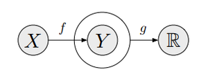
In a traditional supervised learning setting, we are given a training set [math]\displaystyle{ D=\{(x_1, y_1), \cdots, (x_n, y_n)\} }[/math] of [math]\displaystyle{ n }[/math] training examples. Each example is a pair [math]\displaystyle{ (x_i,y_i) }[/math] formed by an instance [math]\displaystyle{ x_i \in X }[/math] and the corresponding output (label) [math]\displaystyle{ y_i \in Y }[/math]. The goal is to learn a function [math]\displaystyle{ f: X \rightarrow Y }[/math] mapping inputs to outputs. To quantify performance, a loss function [math]\displaystyle{ \ell:Y \times Y \rightarrow \mathbb{R} }[/math] is provided, and a mapping is found via
where the optimization is over a pre-defined class of functions [math]\displaystyle{ \mathcal{F} }[/math] (hypothesis class). In our case, [math]\displaystyle{ \mathcal{F} }[/math] will be (convolutional) neural networks parameterized by their weights. The loss could be for example [math]\displaystyle{ \ell(f(x_i),y_i) = 1[f(x_i) \neq y_i] }[/math]. By restricting the space of possible functions specifying the hypothesis class [math]\displaystyle{ \mathcal{F} }[/math], we are leveraging prior knowledge about the specific problem we are trying to solve. Informally, the so-called No Free Lunch Theorems state that every machine learning algorithm must make such assumptions in order to work. Another common way in which a modeler incorporates prior knowledge is by specifying an a-priori preference for certain functions in [math]\displaystyle{ \mathcal{F} }[/math], incorporating a regularization term [math]\displaystyle{ R:\mathcal{F} \rightarrow \mathbb{R} }[/math], and solving for [math]\displaystyle{ f^* = argmin_{f \in \mathcal{F}} \sum_{i=1}^n \ell(f(x_i),y_i) + R(f) }[/math]. Typically, the regularization term [math]\displaystyle{ R:\mathcal{F} \rightarrow \mathbb{R} }[/math] specifies a preference for "simpler" functions (Occam's razor) to prevent overfitting the model on the training data.
The focus is on the set of problems/domains where the problem is a complex environment having a complex representation of the output space, for example mapping an input image to the height of an object(since this leads to a complex output space) rather than simple binary classification problem.
In this paper, prior knowledge on the structure of the outputs is modeled by providing a weighted constraint function [math]\displaystyle{ g:X \times Y \rightarrow \mathbb{R} }[/math], used to penalize “structures” that are not consistent with our prior knowledge. And whether this weak form of supervision is sufficient to learn interesting functions is explored. While one clearly needs labels [math]\displaystyle{ y }[/math] to evaluate [math]\displaystyle{ f^* }[/math], labels may not be necessary to discover [math]\displaystyle{ f^* }[/math]. If prior knowledge informs us that outputs of [math]\displaystyle{ f^* }[/math] have other unique properties among functions in [math]\displaystyle{ \mathcal{F} }[/math], we may use these properties for training rather than direct examples [math]\displaystyle{ y }[/math].
Specifically, an unsupervised approach where the labels [math]\displaystyle{ y_i }[/math] are not provided to us is considered, where a necessary property of the output [math]\displaystyle{ g }[/math] is optimized instead.
If the optimizing the above equation is sufficient to find [math]\displaystyle{ \hat{f}^* }[/math], we can use it in replace of labels. If it's not sufficient, additional regularization terms are added. The idea is illustrated with three examples, as described in the next section.
Experiments
In this paper, the author introduced three contexts to map from inputs to outputs, without providing direct examples of those outputs. In the first two experiments (tracking an object in free fall and tracking the position of a walking man), the author constructed mappings from an image to the location of an object it contains. Learning is made possible by exploiting structure that holds in images over time. In third experiment (detecting objects with causal relationships), the author mapped an image to two boolean variables describing whether or not the image contains two special objects. While learning exploits the unique causal semantics existing between these objects.
Tracking an object in free fall
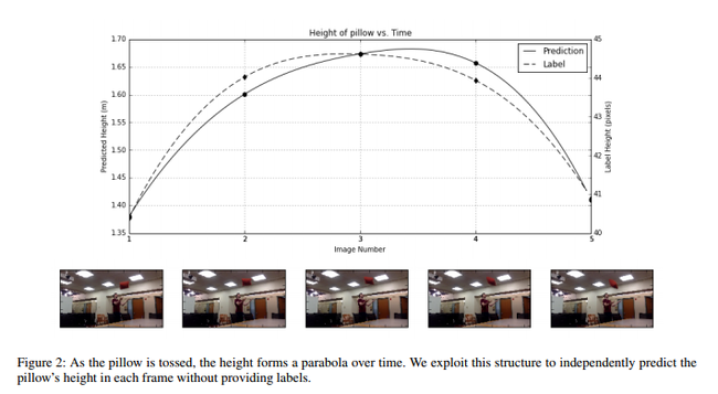
In the first experiment, they record videos of an object being thrown across the field of view, and aim to learn the object's height in each frame. The dataset used as released by the authors can be found at [3]. The goal is to obtain a regression network mapping from [math]\displaystyle{ {R^{\text{height} \times \text{width} \times 3}} \rightarrow \mathbb{R} }[/math], where [math]\displaystyle{ \text{height} }[/math] and [math]\displaystyle{ \text{width} }[/math] are the number of vertical and horizontal pixels per frame, and each pixel has 3 color channels. This network is trained as a structured prediction problem operating on a sequence of [math]\displaystyle{ N }[/math] images to produce a sequence of [math]\displaystyle{ N }[/math] heights, [math]\displaystyle{ \left(R^{\text{height} \times \text{width} \times 3} \right)^N \rightarrow \mathbb{R}^N }[/math], and each piece of data [math]\displaystyle{ x_i }[/math] will be a vector of images, [math]\displaystyle{ \mathbf{x} }[/math]. Rather than supervising the network with direct labels, [math]\displaystyle{ \mathbf{y} \in \mathbb{R}^N }[/math], the network is instead supervised to find an object obeying the elementary physics of free falling objects. An object acting under gravity will have a fixed acceleration of [math]\displaystyle{ a = -9.8 m / s^2 }[/math], and the plot of the object's height over time will form a parabola:
The idea is, given any trajectory of [math]\displaystyle{ N }[/math] height predictions, [math]\displaystyle{ f(\mathbf{x}) }[/math], we fit a parabola with fixed curvature to those predictions, and minimize the resulting residual. Formally, if we specify [math]\displaystyle{ \mathbf{a} = [\frac{1}{2} a\Delta t^2, \frac{1}{2} a(2 \Delta t)^2, \ldots, \frac{1}{2} a(N \Delta t)^2] }[/math], the prediction produced by the fitted parabola is:
By the solution of ordinary least square estimation:
where
[math]\displaystyle{ \mathbf{A} = \left[ {\begin{array}{*{20}c} \Delta t & 1 \\ 2\Delta t & 1 \\ 3\Delta t & 1 \\ \vdots & \vdots \\ N\Delta t & 1 \\ \end{array} } \right] }[/math]
The constraint loss is then defined as
Note that [math]\displaystyle{ \hat{y} }[/math] is not the ground truth labels. Because [math]\displaystyle{ g }[/math] is differentiable almost everywhere, it can be optimized with SGD. They find that when combined with existing regularization methods for neural networks, this optimization is sufficient to recover [math]\displaystyle{ f^* }[/math] up to an additive constant [math]\displaystyle{ C }[/math] (specifying what object height corresponds to 0).

The data set is collected on a laptop webcam running at 10 frames per second ([math]\displaystyle{ \Delta t = 0.1s }[/math]). The camera position is fixed and 65 diverse trajectories of the object in flight, totalling 602 images are recorded. For each trajectory, the network is trained on randomly selected intervals of [math]\displaystyle{ N=5 }[/math] contiguous frames. Images are resized to [math]\displaystyle{ 56 \times 56 }[/math] pixels before going into a small, randomly initialized neural network with no pretraining. The network consists of 3 Conv/ReLU/MaxPool blocks followed by 2 Fully Connected/ReLU layers with probability 0.5 dropout and a single regression output.
Since scaling the [math]\displaystyle{ y_0 }[/math] and [math]\displaystyle{ v_0 }[/math] results in the same constraint loss [math]\displaystyle{ g }[/math], the authors evaluate the result by the correlation of predicted heights with ground truth pixel measurements. This method was used since the distance from the object to the camera could not be accurately recorded, and this distance is required to calculate the height in meters. This is not a bullet proof evaluation, and is discussed in further detail in the critique section. The results are compared to a supervised network trained with the labels to directly predict the height of the object in pixels. The supervised learning task is viewed as a substantially easier task. From this knowledge we can see from the table below that, under their evaluation criteria, the result performs well.
Evaluation
| Method | Random Uniform Output | Supervised with Labels | Approach in this Paper |
|---|---|---|---|
| Correlation | 12.1% | 94.5% | 90.1% |
Tracking the position of a walking man
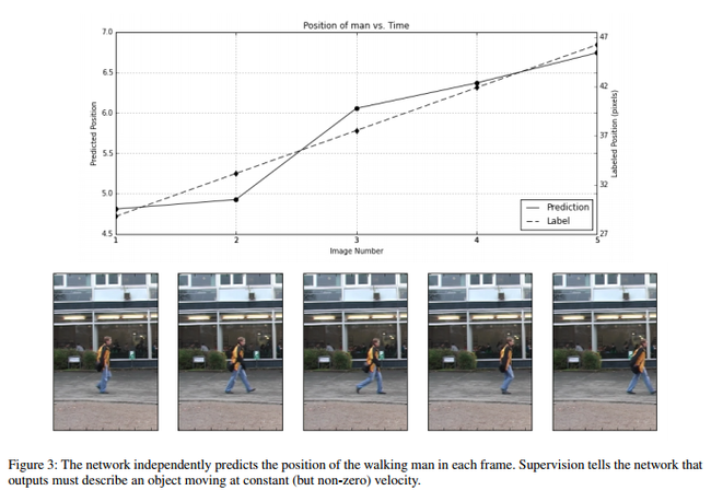
In the second experiment, they aim to detect the horizontal position of a person walking across a frame without providing direct labels [math]\displaystyle{ y \in \mathbb{R} }[/math] by exploiting the assumption that the person will be walking at a constant velocity over short periods of time. This is formulated as a structured prediction problem [math]\displaystyle{ f: \left(R^{\text{height} \times \text{width} \times 3} \right)^N \rightarrow \mathbb{R}^N }[/math], and each training instances [math]\displaystyle{ x_i }[/math] are a vector of images, [math]\displaystyle{ \mathbf{x} }[/math], being mapped to a sequence of predictions, [math]\displaystyle{ \mathbf{y} }[/math]. Given the similarities to the first experiment with free falling objects, we might hope to simply remove the gravity term from equation and retrain. However, in this case, that is not possible, as the constraint provides a necessary, but not sufficient, condition for convergence.
Given any sequence of correct outputs, [math]\displaystyle{ (\mathbf{y}_1, \ldots, \mathbf{y}_N) }[/math], the modified sequence, [math]\displaystyle{ (\lambda * \mathbf{y}_1 + C, \ldots, \lambda * \mathbf{y}_N + C) }[/math] ([math]\displaystyle{ \lambda, C \in \mathbb{R} }[/math]) will also satisfy the constant velocity constraint. In the worst case, when [math]\displaystyle{ \lambda = 0 }[/math], [math]\displaystyle{ f \equiv C }[/math], and the network can satisfy the constraint while having no dependence on the image. The trivial output is avoided by adding two two additional loss terms.
which seeks to maximize the standard deviation of the output, and
[math]\displaystyle{ \begin{split} h_2(\mathbf{x}) = \hphantom{'} & \text{max}(\text{ReLU}(f(\mathbf{x}) - 10)) \hphantom{\text{ }}+ \\ & \text{max}(\text{ReLU}(0 - f(\mathbf{x}))) \end{split} }[/math]
which limit the output to a fixed ranged [math]\displaystyle{ [0, 10] }[/math], the final loss is thus:
[math]\displaystyle{ \begin{split} g(\mathbf{x}) = \hphantom{'} & ||(\mathbf{A} (\mathbf{A}^T\mathbf{A})^{-1} \mathbf{A}^T - \mathbf{I}) * f(\mathbf{x})||_1 \hphantom{\text{ }}+ \\ & \gamma_1 * h_1(\mathbf{x}) \hphantom{\text{ }}+ \\ & \gamma_2 * h_2(\mathbf{x}) % h_2(y) & = \text{max}(\text{ReLU}(y - 10)) + \\ % & \hphantom{=}\hphantom{a} \text{max}(\text{ReLU}(0 - y)) \end{split} }[/math]

The data set contains 11 trajectories across 6 distinct scenes, totalling 507 images resized to [math]\displaystyle{ 56 \times 56 }[/math]. The network is trained to output linearly consistent positions on 5 strided frames from the first half of each trajectory, and is evaluated on the second half. The boundary violation penalty is set to [math]\displaystyle{ \gamma_2 = 0.8 }[/math] and the standard deviation bonus is set to [math]\displaystyle{ \gamma_1 = 0.6 }[/math].
As in the previous experiment, the result is evaluated by the correlation with the ground truth. The result is as follow:
Evaluation
| Method | Random Uniform Output | Supervised with Labels | Approach in this Paper |
|---|---|---|---|
| Correlation | 45.9% | 80.5% | 95.4% |
Surprisingly, the approach in this paper beats the same network trained with direct labeled supervision on the test set, which can be attributed to overfitting on the small amount of training data available (as correlation on training data reached 99.8%).
Detecting objects with causal relationships
In the previous experiments, the authors explored options for incorporating constraints pertaining to dynamics equations in real-world phenomena, i.e., prior knowledge derived from elementary physics. In this experiment, the authors explore the possibilities of learning from logical constraints imposed on single images. More specifically, they ask whether it is possible to learn from causal phenomena.

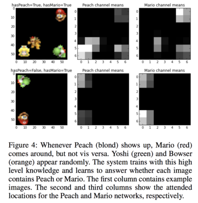
Here, the authors provide images containing a stochastic collection of up to four characters: Peach, Mario, Yoshi, and Bowser, with each character having small appearance changes across frames due to rotation and reflection. Example images can be seen in Fig. (4). While the existence of objects in each frame is non-deterministic, the generating distribution encodes the underlying phenomenon that Mario will always appear whenever Peach appears. The aim is to create a pair of neural networks [math]\displaystyle{ f_1, f_2 }[/math] for identifying Peach and Mario, respectively. The networks, [math]\displaystyle{ f_k : R^{height×width×3} → \{0, 1\} }[/math], map the image to the discrete boolean variables, [math]\displaystyle{ y_1 }[/math] and [math]\displaystyle{ y_2 }[/math]. Rather than supervising with direct labels, the authors train the networks by constraining their outputs to have the logical relationship [math]\displaystyle{ y_1 ⇒ y_2 }[/math]. This problem is challenging because the networks must simultaneously learn to recognize the characters and select them according to logical relationships. To avoid the trivial solution [math]\displaystyle{ y_1 \equiv 1, y_2 \equiv 1 }[/math] on every image, three additional loss terms need to be added:
which forces rotational independence of the outputs in order to encourage the network to learn the existence, rather than location of objects,
which seeks high variance outputs, and
[math]\displaystyle{ h_3(\mathbf{x}, v) = \frac{1}{M}\sum_i^{M} (Pr[f(\mathbf{x}_i) = v] - \frac{1}{3} + (\frac{1}{3} - \mu_v))^2 \\ \mu_{v} = \frac{1}{M}\sum_i^{M} \mathbb{1}\{v = \text{argmax}_{v' \in \{0, 1\}^2} Pr[f(\mathbf{x}) = v']\}. }[/math]
which seeks high entropy outputs. The final loss function then becomes:
[math]\displaystyle{ \begin{split} g(\mathbf{x}) & = \mathbb{1}\{f_1(\mathbf{x}) \nRightarrow f_2(\mathbf{x})\} \hphantom{\text{ }} + \\ & \sum_{k \in \{1, 2\}} \gamma_1 h_1(\mathbf{x}, k) + \gamma_2 h_2(\mathbf{x}, k) + \hspace{-0.7em} \sum_{v \neq \{1,0\}} \hspace{-0.7em} \gamma_3 * h_3(\mathbf{x}, v) \end{split} }[/math]
Evaluation
The input images, shown in Figure 4, are 56 × 56 pixels. The authors used [math]\displaystyle{ \gamma_1 = 0.65, \gamma_2 = 0.65, \gamma_3 = 0.95 }[/math], and trained for 4,000 iterations. This experiment demonstrates that networks can learn from constraints that operate over discrete sets with potentially complex logical rules. Removing constraints will cause learning to fail. Thus, the experiment also shows that sophisticated sufficiency conditions can be key to success when learning from constraints.
Conclusion and Critique
This paper has introduced a method for using physics and other domain constraints to supervise neural networks. However, the approach described in this paper is not entirely new. Similar ideas are already widely used in Q learning, where the Q value are not available, and the network is supervised by the constraint, as in Deep Q learning (Mnih, Riedmiller et al. 2013[2]). In Deep Q-Learning (DQN) also uses a deep neural network which is trained with constraints just like this paper proposes.
Also, the paper has a mistake where they quote the free fall equation as
which should be
Although in this case it doesn't affect the result.
For the evaluation of the experiments, correlation with ground truth was used as the metric to avoid the fact that the output can be scaled without affecting the constraint loss, which is fine if the network gives output of the same scale. However, it is possible that, and the network may give output of varying scale for different inputs, in which case, we have no confidence that the network has learnt correctly, although the learnt outcome may be correlated with ground truth strongly. In fact, to solve the scaling issue, an better approach is to combine the constraints introduced in this paper with some labeled training data. It's not clear why the author didn't experiment with a combination of these two losses.
With regards to the free fall experiment in particular, the authors apply a fixed acceleration model to create the constraint loss, aiming to have the network predict height. However, since they did not measure the true height of the object to create test labels, they evaluate using height in pixel space. They do not mention the accuracy of their camera calibration, nor what camera model was used to remove lens distortion. Since lens distortion tends to be worse at the extreme edges of the image, and that they tossed the pillow throughout the entire frame, it is likely that the ground truth labels were corrupted by distortion. If that is the case, it is possible the supervised network is actually performing worse, because it learning how to predict distorted (beyond a constant scaling factor) heights instead of the true height.
These methods essentially boil down to generating approximate labels for training data using some knowledge of the dynamic that the labels should follow.
Finally, this paper only picks examples where the constraints are easy to design, while in some more common tasks such as image classification, what kind of constraints are needed is not straightforward at all.
Related Work
Constraint learning is a generalization of supervised learning that allows for more creative methods of supervision. For example, multiple-instance learning as proposed by (Dietterich, Lathrop, and Lozano-Pe ́rez 1997; Zhou and Xu 2007) allows for more efficient labeling by providing annotations over groups of images and learning to predict properties that hold over at least one input in a group. In rank learning, labels may given as orderings between inputs with the objective being to find an embedding of inputs that respects the ordering relation (Joachims 2002). Inductive logic programming approaches rely on logical formalisms and constraints to represent background knowledge and learn hypotheses from data (Muggleton and De Raedt 1994; De Raedt 2008; De Raedt and Kersting 2003). Various types of constraints have also been used extensively to guide unsupervised learning algorithms, such as clustering and dimensionality reduction techniques (Lee and Seung 2001; Basu, Davidson, and Wagstaff 2008; Zhi et al. 2013; Ermon et al. 2015).
References
[1] LeCun, Y.; Bengio, Y.; and Hinton, G. 2015. Deep learning. Nature 521(7553):436–444.
[2] Mnih, V.; Kavukcuoglu, K.; Silver, D.; Graves, A.; Antonoglou, I.; Wierstra, D.; and Riedmiller, M. 2013. Playing Atari with Deep Reinforcement Learning. arxiv 1312.5602.
[3] “Russell91/Labelfree.” GitHub, github.com/russell91/labelfree.