Improving neural networks by preventing co-adaption of feature detectors
Presented by
Stan Lee, Seokho Lim, Kyle Jung, Dae Hyun Kim
Improvement Intro
Drop Out Model
In this paper, Hinton et al. introduce a novel way to improve neural networks’ performance, particularly in the case that a large feedforward neural network is trained on a small training set, which causes poor performance and leads to an “overfitting” problem. This problem can be reduced by randomly omitting half of the feature detectors on each training case. In fact, By omitting neurons in hidden layers with a probability of 0.5, each hidden unit is prevented from relying on other hidden units being present during training. Hence there are fewer co-adaptations among them on the training data. Called “dropout,” this process is also an efficient alternative to train many separate networks and average their predictions on the test set.
The intuition for dropout is that if neurons are randomly dropped during training, they can no longer rely on their neighbours, thus allowing each neuron to become more robust. Another interpretation is that dropout is similar to training an ensemble of models since each epoch with randomly dropped neurons can be viewed as its own model.
They used the standard, stochastic gradient descent algorithm and separated training data into mini-batches. An upper bound was set on the L2 norm of incoming weight vector for each hidden neuron, which was normalized if its size exceeds the bound. They found that using a constraint, instead of a penalty, forced the model to do a more thorough search of the weight-space, when coupled with the very large learning rate that decays during training.
Mean Network
Their dropout models included all of the hidden neurons, and their outgoing weights were halved to account for the chances of omission. This is called a 'Mean Network'. This is similar to taking the geometric mean of the probability distribution predicted by all [math]\displaystyle{ 2^N }[/math] networks. Due to this cumulative addition, the correct answers will have a higher log probability than an individual dropout network, which also leads to a lower squared error of the network.
Hidden Markov Models
The Hidden Markov models are used to deal with temporal variability and the models require an acoustic model to determine how well acoustic inputs are fitted to each state of the model. With a neural network with 4 fully-connected hidden layers of 4000 units per layer and 185 "softmax" outputs units that subsequently merge into 39 distinct classes that present in the database. When a dropout rate of 50% is applied, the results improved from 22.5% to 19.7% which sets the record for a model that does not use speaker identity to correct acoustic processing.
The models were shown to result in lower test error rates on several datasets: MNIST; TIMIT; Reuters Corpus Volume; CIFAR-10; and ImageNet.
MNIST
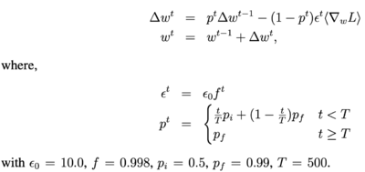
The MNIST dataset contains 70,000 digit images of size 28 x 28. To see the impact of dropout, they used 4 different neural networks (784-800-800-10, 784-1200-1200-10, 784-2000-2000-10, 784-1200-1200-1200-10), with the same dropout rates, 50%, for hidden neurons and 20% for visible neurons. Stochastic gradient descent was used with mini-batches of size 100 and a cross-entropy objective function as the loss function. Weights were updated after each minibatch, and training was done for 3000 epochs. An exponentially decaying learning rate [math]\displaystyle{ \epsilon }[/math] was used, with the initial value set as 10.0, and it was multiplied by the decaying factor [math]\displaystyle{ f }[/math] = 0.998 at the end of each epoch. At each hidden layer, the incoming weight vector for each hidden neuron was set an upper bound of its length, [math]\displaystyle{ l }[/math], and they found from cross-validation that the results were the best when [math]\displaystyle{ l }[/math] = 15. Initial weights values were pooled from a normal distribution with mean 0 and standard deviation of 0.01. To update weights, an additional variable, p, called momentum, was used to accelerate learning. The initial value of [math]\displaystyle{ p }[/math] was 0.5, and it increased linearly to the final value 0.99 during the first 500 epochs, remaining unchanged after. Also, when updating weights, the learning rate was multiplied by [math]\displaystyle{ 1 – p }[/math]. [math]\displaystyle{ L }[/math] denotes the gradient of loss function.
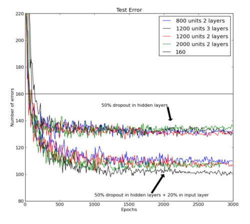
The best-published result for a standard feedforward neural network was 160 errors. This was reduced to about 130 errors with 0.5 dropout and different L2 constraints for each hidden unit input weight. By omitting a random 20% of the input pixels in addition to the aforementioned changes, the number of errors was further reduced to 110. The following figure visualizes the result.
A publicly available pre-trained deep belief net resulted in 118 errors, and it was reduced to 92 errors when the model was fine-tuned with dropout. Another publicly available model was a deep Boltzmann machine, and it resulted in 103, 97, 94, 93 and 88 when the model was fine-tuned using standard backpropagation and was unrolled. They were reduced to 83, 79, 78, 78, and 77 when the model was fine-tuned with dropout – the mean of 79 errors was a record for models that do not use prior knowledge or enhanced training sets.
TIMIT
TIMIT dataset includes voice samples of 630 American English speakers varying across 8 different dialects. It is often used to evaluate the performance of automatic speech recognition systems. Using Kaldi, the dataset was pre-processed to extract input features in the form of log filter bank responses.
Pre-training and Training
For pretraining, they pre-trained their neural network with a deep belief network and the first layer was built using Restricted Boltzmann Machine (RBM) which is a generative stochastic artificial neural network that can learn a probability distribution over its set of inputs. Initializing visible biases with zero, weights were sampled from random numbers that followed normal distribution [math]\displaystyle{ N(0, 0.01) }[/math]. Each visible neuron’s variance was set to 1.0 and remained unchanged.
Minimizing Contrastive Divergence (CD) was used to facilitate learning. Since momentum is used to speed up learning, it was initially set to 0.5 and increased linearly to 0.9 over 20 epochs. The average gradient had 0.001 of a learning rate which was then multiplied by [math]\displaystyle{ (1-momentum) }[/math] and L2 weight decay was set to 0.001. After setting up the hyperparameters, the model was done training after 100 epochs. Binary RBMs were used for training all subsequent layers with a learning rate of 0.01. Then, [math]\displaystyle{ p }[/math] was set as the mean activation of a neuron in the data set and the visible bias of each neuron was initialized to [math]\displaystyle{ log(p/(1 − p)) }[/math]. Training each layer with 50 epochs, all remaining hyper-parameters were the same as those for the Gaussian RBM.
Dropout tuning
The initial weights were set in a neural network from the pre-trained RBMs. To finetune the network with dropout-backpropagation, momentum was initially set to 0.5 and increased linearly up to 0.9 over 10 epochs. The model had a small constant learning rate of 1.0 and it was used to apply to the average gradient on a minibatch. The model also retained all other hyperparameters the same as the model from MNIST dropout finetuning. The model required approximately 200 epochs to converge. For comparison purposes, they also finetuned the same network with standard backpropagation with a learning rate of 0.1 with the same hyperparameters.
Classification Test and Performance
A Neural network was constructed to output the classification error rate on the test set of TIMIT dataset. They have built the neural network with four fully-connected hidden layers with 4000 neurons per layer. The output layer distinguishes distinct classes from 185 softmax output neurons that are merged into 39 classes. After constructing the neural network, 21 adjacent frames with an advance of 10ms per frame was given as an input.
Comparing the performance of dropout with standard backpropagation on several network architectures and input representations, dropout consistently achieved lower error and cross-entropy. Results showed that it significantly controls overfitting, making the method robust to choices of network architecture. It also allowed much larger nets to be trained and removed the need for early stopping. Thus, neural network architectures with dropout are not very sensitive to the choice of learning rate and momentum.
Reuters Corpus Volume
Reuters Corpus Volume I archives 804,414 news documents that belong to 103 topics. Under four major themes - corporate/industrial, economics, government/social, and markets – they belonged to 63 classes. After removing 11 classes with no data and one class with insufficient data, they are left with 50 classes and 402,738 documents. The documents were divided into training and test sets equally and randomly, with each document representing the 2000 most frequent words in the dataset, excluding stopwords.
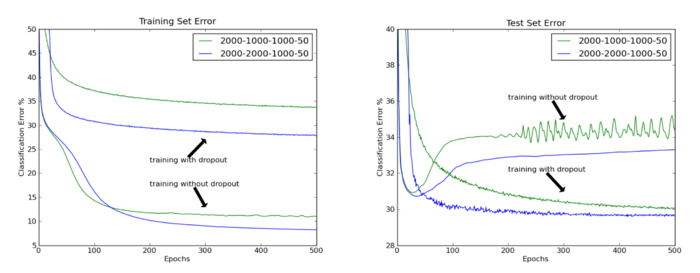
They trained two neural networks, with size 2000-2000-1000-50, one using dropout and backpropagation, and the other using standard backpropagation. The training hyperparameters are the same as that in MNIST, but training was done for 500 epochs.
In the following figure, we see the significant improvements by the model with dropout in the test set error. On the right side, we see that learning with dropout also proceeds smoother.
CNN
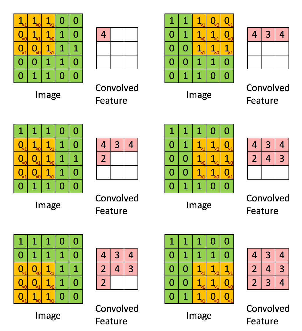
Feed-forward neural networks consist of several layers of neurons where each neuron in a layer applies a linear filter to the input image data and is passed on to the neurons in the next layer. When calculating the neuron’s output, scalar bias a.k.a weights are applied to the filter with nonlinear activation function as parameters of the network that are learned by training data.
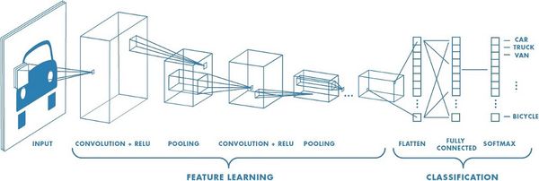
There are several differences between Convolutional Neural networks and ordinary neural networks. The figure above gives a visual representation of a Convolutional Neural Network. First, CNN’s neurons are organized topographically into a bank and laid out on a 2D grid, so it reflects the organization of dimensions of the input data. Secondly, neurons in CNN apply filters which are local, and which are centered at the neuron’s location in the topographic organization. Meaning that useful metrics or clues to identify the object in an input image can be found by examining local neighborhoods of the image. Next, all neurons in a bank apply the same filter at different locations in the input image. When looking at the image example, green is input to one neuron bank, yellow is a filter bank, and pink is the output of one neuron bank (convolved feature). A bank of neurons in a CNN applies a convolution operation, aka filters, to its input where a single layer in a CNN typically has multiple banks of neurons, each performing a convolution with a different filter. The resulting neuron banks become distinct input channels into the next layer. The whole process reduces the net’s representational capacity but also reduces the capacity to overfit.
Pooling
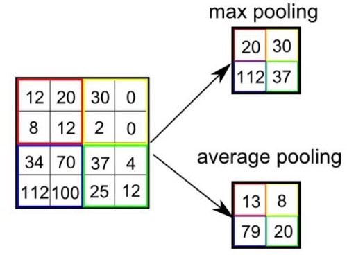
Pooling layer summarizes the activities of local patches of neurons in the convolutional layer by subsampling the output of a convolutional layer. Pooling is useful for extracting dominant features, to decrease the computational power required to process the data through dimensionality reduction. The procedure of pooling goes on like this; output from convolutional layers is divided into sections called pooling units and they are laid out topographically, connected to a local neighborhood of other pooling units from the same convolutional output. Then, each pooling unit is computed with some function which could be maximum and average. Maximum pooling returns the maximum value from the section of the image covered by the pooling unit while average pooling returns the average of all the values inside the pooling unit (see example). In the result, there are fewer total pooling units than convolutional unit outputs from the previous layer, this is due to the larger spacing between pixels on pooling layers. Using the max-pooling function reduces the effect of outliers and improves generalization. Other than that, overlapping pooling makes this spacing between pixels smaller than the size of the neighborhood that the pooling units summarize (This spacing is usually referred to as the stride between pooling units). With this variant, pooling layer can produce a coarse coding of the outputs which helps generalization.
Local Response Normalization
This network includes local response normalization layers which are implemented in lateral form and used on neurons with unbounded activations and permit the detection of high-frequency features with a big neuron response. This regularizer encourages competition among neurons belonging to different banks. Normalization is done by dividing the activity of a neuron in bank [math]\displaystyle{ i }[/math] at position [math]\displaystyle{ (x,y) }[/math] by the equation:

where the sum runs over [math]\displaystyle{ N }[/math] ‘adjacent’ banks of neurons at the same position as in the topographic organization of neuron bank. The constants, [math]\displaystyle{ N }[/math], [math]\displaystyle{ alpha }[/math] and [math]\displaystyle{ betas }[/math] are hyper-parameters whose values are determined using a validation set. This technique is replaced by better techniques such as the combination of dropout and regularization methods ([math]\displaystyle{ L1 }[/math] and [math]\displaystyle{ L2 }[/math])
Neuron nonlinearities
All of the neurons for this model use the max-with-zero nonlinearity where output within a neuron is computed as [math]\displaystyle{ a^{i}_{x,y} = max(0, z^i_{x,y}) }[/math] where [math]\displaystyle{ z^i_{x,y} }[/math] is the total input to the neuron. The reason they use nonlinearity is that it has several advantages over traditional saturating neuron models, such as a significant reduction in training time required to reach a certain error rate. Another advantage is that nonlinearity reduces the need for contrast-normalization and data pre-processing since neurons do not saturate- meaning activities simply scale up little by little with usually large input values. For this model’s only pre-processing step, they subtract the mean activity from each pixel and the result is a centered data.
Objective function
The objective function of their network maximizes the multinomial logistic regression objective which is the same as minimizing the average cross-entropy across training cases between the true label and the model’s predicted label.
Weight Initialization
It’s important to note that if a neuron always receives a negative value during training, it will not learn because its output is uniformly zero under the max-with-zero nonlinearity. Hence, the weights in their model were sampled from a zero-mean normal distribution with a high enough variance. High variance in weights will set a certain number of neurons with positive values for learning to happen, and in practice, it’s necessary to try out several candidates for variances until a working initialization is found. In their experiment, setting a positive constant, or 1, as biases of the neurons in the hidden layers was helpful in finding it.
Training
In this model, a batch size of 128 samples and momentum of 0.9, we train our model using stochastic gradient descent. The update rule for weight [math]\displaystyle{ w }[/math] is $$ v_{i+1} = 0.9v_i + \epsilon <\frac{dE}{dw_i}> i$$ $$w_{i+1} = w_i + v_{i+1} $$ where [math]\displaystyle{ i }[/math] is the iteration index, [math]\displaystyle{ v }[/math] is a momentum variable, [math]\displaystyle{ \epsilon }[/math] is the learning rate and [math]\displaystyle{ \frac{dE}{dw} }[/math] is the average over the [math]\displaystyle{ i }[/math]th batch of the derivative of the objective with respect to [math]\displaystyle{ w_i }[/math]. The whole training process on CIFAR-10 takes roughly 90 minutes and ImageNet takes 4 days with dropout and two days without.
Learning
To determine the learning rate for the network, it is a must to start with an equal learning rate for each layer which produces the largest reduction in the objective function with the power of ten. Usually, it is in the order of [math]\displaystyle{ 10^{-2} }[/math] or [math]\displaystyle{ 10^{-3} }[/math]. In this case, they reduce the learning rate twice by a factor of ten before the termination of training.
CIFAR-10
CIFAR-10 Dataset
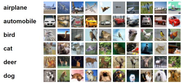
Removing incorrect labels, The CIFAR-10 dataset is a subset of the Tiny Images dataset with 10 classes. It contains 5000 training images and 1000 testing images for each class. The dataset has 32 x 32 color images searched from the web and the images are labeled with the noun used to search the image.
Models for CIFAR-10
Two models, one with dropout and one without dropout, were built to test the performance of dropout on CIFAR-10. All models have CNN with three convolutional layers each with a pooling layer. All of the pooling payers use a stride=2 and summarize a 3*3 neighborhood. The max-pooling method is performed by the pooling layer which follows the first convolutional layer, and the average-pooling method is performed by the remaining 2 pooling layers. The first and second pooling layers with [math]\displaystyle{ N = 9, α = 0.001 }[/math], and [math]\displaystyle{ β = 0.75 }[/math] are followed by response normalization layers. A ten-unit softmax layer, which is used to output a probability distribution over class labels, is connected with the upper-most pooling layer. Using a filter size of 5×5, all convolutional layers have 64 filter banks.
Additional changes were made with the model with dropout. The model with dropout enables us to use more parameters because dropout forces a strong regularization on the network. Thus, a fourth weight layer is added to take the input from the previous pooling layer. This fourth weight layer is locally connected, but not convolutional, and contains 16 banks of filters of size 3 × 3 with 50% dropout. Lastly, the softmax layer takes its input from this fourth weight layer.
Thus, with a neural network with 3 convolutional hidden layers with 3 max-pooling layers, the classification error achieved 16.6% to beat 18.5% from the best-published error rate without using transformed data. The model with one additional locally-connected layer and dropout at the last hidden layer produced an error rate of 15.6%.
ImageNet
ImageNet Dataset
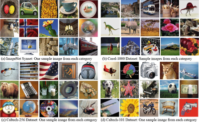
ImageNet is a dataset of millions of high-resolution images, and they are labeled among 1000 different categories. The data were collected from the web and manually labeled using MTerk tool, which is a crowd-sourcing tool provided by Amazon. Because this dataset has millions of labeled images in thousands of categories, it is very difficult to have perfect accuracy on this dataset even for humans because the ImageNet images may contain multiple objects and there are a large number of object classes. ImageNet and CIFAR-10 are very similar, but the scale of ImageNet is about 20 times bigger (1,300,000 vs 60,000). The size of ImageNet is about 1.3 million training images, 50,000 validation images, and 150,000 testing images. They used resized images of 256 x 256 pixels for their experiments.
An ambiguous example to classify:

When this paper was written, the best score on this dataset was the error rate of 45.7% by High-dimensional signature compression for large-scale image classification (J. Sanchez, F. Perronnin, CVPR11 (2011)). The authors of this paper could achieve a comparable performance of 48.6% error rate using a single neural network with five convolutional hidden layers with a max-pooling layer in between, followed by two globally connected layers and a final 1000-way softmax layer. When applying 50% dropout to the 6th layer, the error rate was brought down to 42.4%.
ImageNet Dataset:
Models for ImageNet
They mostly focused on the model with dropout because the one without dropout had a similar approach, but there was a serious issue with overfitting. They used a convolutional neural network trained by 224×224 patches randomly extracted from the 256 × 256 images. This could reduce the network’s capacity to overfit the training data and helped generalization as a form of data augmentation. The method of averaging the prediction of the net on ten 224 × 224 patches of the 256 × 256 input image was used for testing their model patched at the center, four corners, and their horizontal reflections. To maximize the performance on the validation set, this complicated network architecture was used and it was found that dropout was very effective. Also, it was demonstrated that using non-convolutional higher layers with the number of parameters worked well with dropout, but it had a negative impact on the performance without dropout.
The network contains seven weight layers. The first five are convolutional, and the last two are globally-connected. Max-pooling layers follow the layer number 1,2, and 5. And then, the output of the last globally-connected layer was fed to a 1000-way softmax output layer. Using this architecture, the authors achieved an error rate of 48.6%. When applying 50% dropout to the 6th layer, the error rate was brought down to 42.4%.
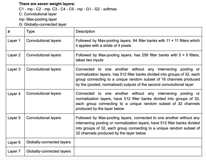
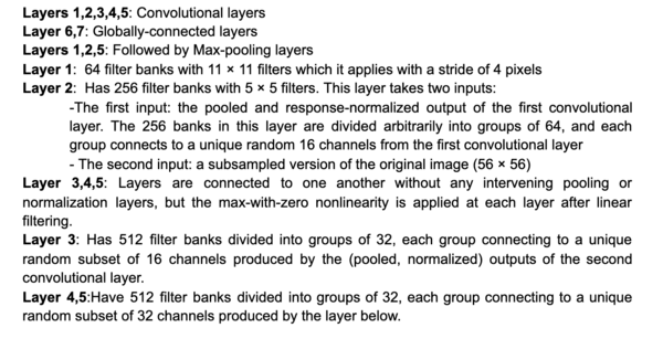
Like the previous datasets, such as the MNIST, TIMIT, Reuters, and CIFAR-10, we also see a significant improvement for the ImageNet dataset. Including complicated architectures like this one, introducing dropout generalizes models better and gives lower test error rates.
Conclusion
The authors have shown a consistent improvement by the models trained with dropout in classifying objects in the following datasets: MNIST; TIMIT; Reuters Corpus Volume I; CIFAR-10; and ImageNet.
The authors comment on a theory that sexual reproduction limits biological function to a small number of coadapted genes. The idea is that a given organism is unlikely to receive many coordinated genes from a parent, so will likely die if it relies on many genes to perform a given task. This limits the number of genes required to perform a function, which is like a built-in evolutionary dropout.
Critiques
It is a very brilliant idea to dropout half of the neurons to reduce co-adaptations. It is mentioned that for fully connected layers, dropout in all hidden layers works better than dropout in only one hidden layer. There is another paper Dropout: A Simple Way to Prevent Neural Networks from Overfitting[1] gives a more detailed explanation.
It will be interesting to see how this paper could be used to prevent the overfitting of LSTMs.
This paper focused more on CV tasks, it will be interesting to have some discussion on NLP tasks
Firstly, it is a very interesting topic of classification by the "dropout" CNN method(omitting neurons in hidden layers). If the author can briefly explain the advantages of this method in processing image data in theory, it will be easier for readers to understand. Also, how to deal with the overfitting issue would be valuable.
The authors mention that they tried various dropout probabilities and that the majority of them improved the model's generalization performance, but that more extreme probabilities tended to be worse which is why a dropout rate of 50% was used in the paper. The authors further develop this point to mention that the method can be improved by adapting individual dropout probabilities of each hidden or input unit using validation tests. This would be an interesting area to further develop and explore, as using a hardcoded 50% dropout for all layers might not be the optimal choice for all CNN applications. It would have been interesting to see the results of their investigations of differing dropout rates.
The authors don't explain that during training, at each layer that we apply dropout, the values must be scaled by 1/p where p is dropout rate - this way the expected value of the layers is the same in both train and test time. They may have considered another solution for this discrepancy at the time (it is an old paper) but it doesn't seem like any solution was presented here.
Despite the advantages of using dropout to prevent overfitting and reducing errors in testing, the authors did not discuss much the effects on the length of training time. In another paper published a few years later by the same authors, there was more discussion about this. It appears that dropout increases training time by 2-3 times compared to a standard NN with the same architecture, which is a drawback that might be worth mentioning.
Dropout layers prevent overfitting by random dropout of a fraction of the neurons specified in each layer. In fact, the neurons to be dropped out in each layer are randomly selected. Therefore, it might be the case that some important features in the dropout layer are discarded, which leads to a sudden drop in performance. Although this barely happens, and CNN with dropout rates roughly 50% in each layer will lead to generally good performance, some future improvements are still possible if we are able to select dropout neurons cleverly.
The article does a good job of analyzing the benefit of using the standard dropout method, but I think it would be beneficial to take a look at other dropout variants. For example, the paper may have benefited from looking at DropConnect which was introduced y L. Wan et al and is similar to dropout layers but it does not apply a dropout directly o the neurons but on the weights and the bias linking the neurons. Others that they also could have looked at were Standout, Pooling Drop and MaxDrop. Comparing various dropout methods I think would greatly add to the paper.
The author analyzed the dropout method for addressing overfitting problems. The key idea is to randomly drop units from the neural network during training. This prevents units from co-adapting too much. In addition, it also fastens the speed of training models since there are fewer neurons, which is a good idea.
Random dropping was indeed quite effective in the MNIST fashion classification challenge, however, it may pose a question if the problem has very few features to begin with.
The authors mentioned that they used Momentum to speed up the training but didn't show the alternative and the speed of the alternative. This paperconducts an empirical study of Dropout vs Batch Normalization as well as compares different optimizers (like SGD which uses momentum) for each technique. It is found that optimizers with momentum outperform adaptive optimizers but at a cost of significantly longer training times.
Dropout is a very popular technique to improve accuracy by avoiding overfitting. It might be interesting to see how it compares to other techniques and how the combination of techniques works.
Dropout is really popular, but its usefulness is oftentimes inversely proportional to the amount of data in the training data, making it less useful for many modern applications. This paper could talk a little more about alternate methods, such as data augmentation, or L1/L2 regularization, and present them as viable alternatives.
Dropout rates often vary across layers, the author does not specify which layers are applied to the dropout layer nor the team explains which layers applied are more important than others. The team gave concrete testing results against other models using many standard tests to show the effectiveness of such a method. However, there is no particular visualization (graphs) against other models in terms of efficiency when a standard training epoch, data split, preprocessing or training/testing loss.
According to the provided frame classification error rate on the core test set of the TIMIT benchmark plot, dropout of 50% of the hidden units and 20% of the input units significantly improves classification. As the plot shown, the curve for finetuning without dropout took a very early turn at epoch size approximately 20, and then maintained very high classification error rate as epoch size increases. The curve for finetuning with dropout kept low no matter the size of epoch after roughly 50, but it fluctuates a lot harder than the curve without dropout, indicating that it has a higher sensitivity in response to epoch size.
Other Work
In modern training, dropout is not advised for convolutional neural networks because it does not have the effect, interpretation, impact on spatial feature maps as dense features. This is because features in CNNs are spatially correlated. There is an interesting paper on DropBlock [2], a dropout method that drops entire contiguous regions of features, which has been shown to be much more effective for CNNs.
Reference
[1] N. Srivastave, "Dropout: a simple way to prevent neural networks from overfitting", The Journal of Machine Learning Research, Jan 2014.
[2] Ghiasi, Golnaz and Lin, Tsung-Yi and Le, Quoc V. "DropBlock: A regularization method for convolutional networks". NeurIPS, 2018.