Summary of the paper: Hierarchical Representations for Efficient Architecture Search

Introduction

Deep Neural Networks (DNNs) have shown remarkable performance in several areas such as computer vision, natural language processing, among others; however, improvements over previous benchmarks have required extensive research and experimentation by domain experts. In DNNs, the composition of linear and nonlinear functions produce internal representations of data which are in most cases better than handcrafted ones; consequently, researchers using Deep Learning techniques have lately shifted their focus from working on input features to designing optimal DNN architectures. However, the quest for finding an optimal DNN architecture by combining layers and modules requires frequent trial and error experiments, a task that resembles the previous work on looking for handcrafted optimal features. As researchers aim to solve more difficult challenges the complexity of the resulting DNN is also increasing; therefore, some studies are introducing the use of automated techniques focused on searching for optimal architectures. The latest emerging field, Neural Architecture Search, is aimed to tackle exactly this problem. The goal of Neural Architecture Search is to try to transform the problem of designing a network into a search problem. For a search problem, it needs a clear definition of three things: the search space, the search strategy, and performance evaluation strategy. The search space is a high-level description of the architecture of the network. The search space needs to contain enough freedom such that the resulted model will have enough expressive power, but cannot be too broad thus makes the search process too computational consuming. The search strategy is how to efficiently search in the search space. The performance evaluation strategy is the methods that are used to evaluate the network. Here, the evaluation is more tricky because in order to evaluate a neural network, we need to train it first, and training takes time. So it is important to define a proxy task that can help us better evaluate a network. Here, this paper will tackle these problems with a new hierarchical representation.

Lately, the use of algorithms for finding optimal DNN architectures has attracted the attention of researchers who have tackled the problem through four main groups of techniques. The first such method employs a supplementary network called a “Hypernet”, which generates ideal network weights given a random architecture. There are two main parts to generating an “optimal” architecture. First, we train the HyperNet. One training cycle consists of generating a random architecture from a sample space of allowed architectures and generating its predicted weights with the HyperNet. Then, the validation score of this proposed network is calculated, and the error is used to backpropagate through the HyperNet. In this manner, the HyperNet can learn to assign robustly optimal initial weights to a given architecture. At “test” time, we generate a random sample of architectures and predict initialized weights for each with our tuned HyperNet. We take the model with the highest validation score and train it as we would a regular architecture. We use this heuristic of “initial validation error” as the relative performance of networks typically stays constant throughout training. That is, if it starts off better, it will very likely end better. The second technique is Monte Carlo Tree Search (MCTS) which repeatedly narrows the search space by focusing on the most promising architectures previously seen. The third group of techniques use evolutionary algorithms where fitness criteria are applied to filter the initial population of DNN candidates, then new individuals are added to the population by selecting the best-performing ones and modifying them with one or several random mutations as in [Real, 2017]. The fourth and last group of techniques implement Reinforcement Learning where a policy based controller seeks to optimize the expected accuracy of new architectures based on rewards (accuracy) gained from previous proposals in the architecture space. From these four groups of techniques, Reinforcement Learning has offered the best experimental results; however, the paper we are summarizing implements evolutionary algorithms as its main approach.

Despite the technique used to look for an optimal architecture, searching in the architecture space usually requires the training and evaluation of many DNN candidates; therefore, it demands huge computational resources and poses a significant limitation for practical applications. Consequently, most techniques narrow the search space with predefined heuristics, either at the beginning or dynamically during the searching process. In the paper we are summarizing, the authors reduce the number of feasible architectures by forcing a hierarchical structure between network components. In other words, each DNN suggested as a candidate is formed by combining basic building blocks to form small modules, then the same basic structures introduced on the building blocks are used to combine and stack networks on the upper levels of the hierarchy. This approach allows the searching algorithm to sample highly complex and modularized networks similar to Inception or ResNet.

Despite some weaknesses regarding the efficiency of evolutionary algorithms, this study reveals that in fact, these techniques can generate architectures which show competitive performance when a narrowing strategy is imposed over the search space. Accordingly, the main contributions of this paper is a well-defined set of hierarchical representations which acts as the filtering criteria to pick DNN candidates and a novel evolutionary algorithm which produces image classifiers that achieve state of the art performance among similar evolutionary-based techniques.

Architecture representations

Flat architecture representation

All the evaluated network architectures are directed acyclic graphs with only one source and one sink. Each node in the network represents a feature map and consequently, each directed edge represents an operation that takes the feature map in the departing node as input and outputs a feature map on the arriving node. Under the previous assumption, any given architecture in the narrowed search space is formally expressed as a graph assembled by a series of operations (edges) among a defined set of adjacent feature maps (nodes).

Multiple primitive operations defined in section 2.3 are used to form small networks defined as motifs by the authors. To combine the outputs of multiple primitive operations and guarantee a unique output per motif the authors introduce a merge operation which in practice works as a depthwise concatenation that does not require inputs with the same number of channels.

Accordingly, these motifs can also be combined to form more complex motifs on a higher level in the hierarchy until the network is complex enough to perform competitively in challenging classification tasks.

Hierarchical architecture representation

The composition of more complex motifs based on simpler motifs at lower levels allows the authors to create a hierarchy-like representation of very complex DNN starting with only a few primitive operations as shown in Figure 1. In other words, an architecture with [math]\displaystyle{ L }[/math] levels has only primitive operations at its bottom and only one complex motif at its top. Any motif in between the bottom and top levels can be defined as the composition of motifs in lower levels of the hierarchy.

Formally, the [math]\displaystyle{ m }[/math]-th motif in level [math]\displaystyle{ l }[/math], [math]\displaystyle{ o_m^{(l)} }[/math], is recursively defined as the composition of lower-level motifs [math]\displaystyle{ \textbf{o}^{(l-1)} }[/math] according to its network structure.

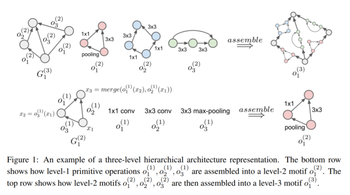
[math]\displaystyle{ o_m^{(l)}=assemble(G_m^{(l)}, \textbf{o}^{(l-1)}) }[/math]

Figure 1. Hierarchical architecture representation

In figure 1, the architecture of the full model (its flat structure) is shown in the top right corner. The input (source) is the bottom-most node. The output (sink) is the topmost node. The paper presents an alternative hierarchical view of the model shown on the left-hand side (before the assemble function). This view represents the same model in three layers. The first layer is a set of primitive operations only (bottom row, middle column). In all other layers component motifs (computational graphs) G are described by an adjacency matrix and a set of operations. The set of operations are from the previous layer. An example motif [math]\displaystyle{ G^{(2)}_{1} }[/math] in the second layer is shown in the bottom row (left and middle columns). There are three unique motifs in the second layer. These are shown in the middle layer of the top row. Note that the motifs in the previous layer become the operations in the next layer. The higher layer can use these motifs multiple times. Finally, the top level graph, which contains only one motif, [math]\displaystyle{ G^{(3)}_{1} }[/math], is shown in the top row left column. Here, there are 4 nodes with 6 operations defined between them.

Primitive operations

The six primitive operations used as building blocks for connecting nodes in either flat or hierarchical representations are:

1 × 1 convolution of C channels
3 × 3 depthwise convolution
3 × 3 separable convolution of C channels
3 × 3 max-pooling
3 × 3 average-pooling
Identity mapping

The authors argue that convolution operations involving larger receptive fields can be obtained by the composition of lower-level motifs with smaller receptive fields. Accordingly, convolution operations considering a large number of channels can be generated by the depthwise concatenation of lower-level motifs. Batch normalization and ReLU activation function are applied after each convolution in the network. There is a seventh operation called null and is used in the adjacency matrix [math]\displaystyle{ G }[/math] to state explicitly that there are no operations between two nodes.

Side note:

Some explanations for different types for convolution:

Spatial convolution: Convolutions performed in spatial dimensions - width and height.
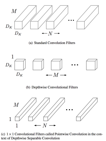
Depthwise convolution: Spatial convolution performed independently over each channel of an input.
1x1 convolution: Convolution with the kernel of size 1x1

Evolutionary architecture search

Before moving forward we introduce the concept of genotypes in the context of the article. In this article, a genotype is a particular neural network architecture defined according to the components described in section 2. In order to make the NN architectures evolve the authors implemented a three stages process that includes establishing the permitted mutations, creating an initial population and make them compete in a tournament where only the best candidates will survive.

Mutation

One mutation over a specific architecture is a sequence of five changes in the following order:

Sample a level in the hierarchy, different than the basic level.
Sample a motif in that level.
Sample a successor node [math]\displaystyle{ (i) }[/math] in the motif.
Sample a predecessor node [math]\displaystyle{ (j) }[/math] in the motif.
Replace the current operation between nodes [math]\displaystyle{ i }[/math] and [math]\displaystyle{ j }[/math] from one of the available operations.

The original operation between the nodes [math]\displaystyle{ i }[/math] and [math]\displaystyle{ j }[/math] in the graph is defined as [math]\displaystyle{ [G_{m}^{\left ( l \right )}] _{ij} = k }[/math]. Therefore, a mutation between the same pair of nodes is defined as [math]\displaystyle{ [G_{m}^{\left ( l \right )}] _{ij} = {k}' }[/math].

The allowed mutations include:

Change the basic primitive between the predecessor and successor nodes (ie. alter an existing edge): if [math]\displaystyle{ o_k^{(l-1)} \neq none }[/math] and [math]\displaystyle{ o_{k'}^{(l-1)} \neq none }[/math] and [math]\displaystyle{ o_{k'}^{(l-1)} \neq \gt o_k^{(l-1)} }[/math]
Add a connection between two previously unconnected nodes. The connection between the node can have any of the six possible primitives: if [math]\displaystyle{ o_k^{(l-1)}=none }[/math] and [math]\displaystyle{ o_{k'}^{(l-1)} \neq none }[/math]
Remove a connection between existing nodes: if [math]\displaystyle{ o_k^{(l-1)} \neq none }[/math] and [math]\displaystyle{ o_{k'}^{(l-1)} = none }[/math]

Initialization

An initial population is required to start the evolutionary algorithm; therefore, the authors introduced a trivial genotype (candidate solution, the hierarchical architecture of the model) composed only of identity mapping operations. Then a large number of random mutations was run over the trivial genotype to simulate a diversification process. The authors argue that this diversification process generates a representative population in the search space and at the same time prevents the use of any handcrafted NN structures. Surprisingly, some of these random architectures show a performance comparable to the performance achieved by the architectures found later during the evolutionary search algorithm.

Search algorithms

Tournament selection and random search are the two search algorithms used by the authors.

Tournament Selection

In one iteration of the tournament selection algorithm, 5% of the entire population is randomly selected, trained, and evaluated against a validation set. Then the best performing genotype is picked to go through the mutation process and put back into the population. No genotype is ever removed from the population, but the selection criteria guarantee that only the best performing models will be selected to evolve through the mutation process.

We define the pseudocode for tournament selection as follows:

1. Choose k (the tournament size) individuals from the population at random

2. Choose the best individual from the tournament with probability p

3. Choose the second best individual with probability p*(1-p)

4. Choose the third best individual with probability p*((1-p)^2)

5. Continue until the number of selected individuals equal the number we desire.

Tournament selection is often chosen over alternative genetic algorithms due to the following benefits: it is efficient to code, works on parallel architectures and allows the selection pressure to be easily adjusted.

Random Search

In the random search algorithm every genotype from the initial population is trained and evaluated, then the best performing model is selected. In contrast to the tournament selection algorithm, the random search algorithm is much simpler and the training and evaluation process for every genotype can be run in parallel to reduce search time. This algorithm is not widely studied in the literature yet.

Implementation

To implement the tournament selection algorithm two auxiliary algorithms are introduced. The first is called the controller and directs the evolution process over the population, in other words, the controller repeatedly picks 5% of genotypes from the current population, send them to the tournament and then apply a random mutation over the best performing genotype from each group.

The second auxiliary algorithm is called the worker and is in charge of training and evaluating each genotype, a task that must be completed each time a new genotype is created and added to the population either by an initialization step or by an evolutionary step.

Both auxiliary algorithms work together asynchronously and communicate each other through a shared tabular memory file where genotypes and their corresponding fitness are recorded.

Experiments and results

Experimental setup

Instead of a looking for a complete NN model, the search framework introduced in section 2 is applied to look for the best performing architectures of a small neural network module called the convolutional cell. Using small modules as building blocks to form a larger and more complex model is an approach proved to be successful in previous cases such as the Inception architecture. Additionally, this approach allowed the authors to evaluate cell candidates efficiently and scale to larger and more complex models faster.

In total three models were implemented as hosts for the experimental cells, the first two use the CIFAR-10 dataset and the third uses the ImageNet dataset. The search framework is implemented only in the first host model to look for the best performing cells (section 4.2), once found, these cells were inserted into the second and third host models to evaluate overall performance on the respective datasets (section 4.3).

The terms training time step, initialization time step, and evolutionary time step will be used to describe some parts of the experiments. Be aware that these three terms have different meanings; however, each term will be properly defined when introduced.

Architecture search on CIFAR-10

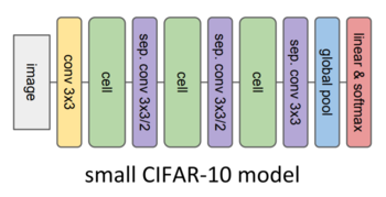
The overall goal in this stage is to find the best performing cells. The search framework is run using the small CIFAR-10 depicted in Figure 2 as host model for the cells; therefore, during the searching process, only the cells change while the rest of the host model’s structure remains the same. In the context of the evolutionary search algorithm, a cell is also called a candidate or a genotype. Additionally, on every time step during the search process, the three cells in the model will share the same structure and consequently every time a new candidate architecture is evaluated the three cells will simultaneously adopt the new candidate’s architecture.

To begin the architecture searching process an initial population of genotypes is required. Random mutations are applied over a trivial genotype to generate a candidate and grow the seminal population. This is called an initialization step and is repeated 200 times to produce an equivalent number of candidates. Creating these 200 candidates with random structures is equivalent to running a random search over a constrained architecture space.

Then, the evolutionary search algorithm takes over and runs from timestep 201 up to time step 7000, these are called evolutionary timesteps. On each evolutionary time step, a group of genotypes equivalent to 5% of the current population is selected randomly and sent to the tournament for fitness computation. To perform a fitness evaluation each candidate cell is inserted into the three predefined positions within the small CIFAR-10 host model. Then for each candidate cell, the host model is trained with stochastic gradient descent during 5000 training steps and decreasing learning rate. Due to observing a standard deviation of up to 0.2% when evaluating the exact same model, the overall fitness is obtained as the average of four training-evaluation runs. This variance is due to optimization. Finally, a random mutation is applied over a copy of the best cell within the group to create a new genotype that is added to the current population.

The fitness of each evaluated genotype is recorded in the shared tabular memory file to avoid recalculation in case the same genotype is selected again in a future evolutionary time step.

The search framework is run for 7000-time steps (200 initialization time steps and the rest are evolutionary time steps) for each one of three different types of cell architecture, namely hierarchical representation, flat representation and flat representation with constrained parameters.

A cell that follows a hierarchical representation has NN connections at three different levels; at the bottom level it has only primitive operations, at the second level it contains motifs with four-nodes and at the third level it has only one motif with five-nodes.

A cell that follows a flat representation has 11 nodes with only primitive operations between them. These cells look similar to level 2 motifs but instead of having four nodes they have 11 and therefore many more pairs of nodes and operations.

For a cell that follows a flat representation with constrained parameters the total number of parameters used by its operations cannot be superior to the total number of parameters used by the cells that follow a hierarchical representation.

Figure 3 shows the current fitness achieved by the best performing cell from each one of the three types of cells when plugged in the small CIFAR-10 model. Even though the fitness grows rapidly after the first 200 (initialization) time steps, it tends to plateau between 89% to 90%. Overall, cells that follow a flat representation without restriction in the number of parameters tend to perform better than those following a hierarchical structure. It could be due to the fact that the flat representation allows more flexibility when adding connections between nodes, especially between distant ones. Unfortunately, the authors do not describe the architecture of the best performing flat cell.

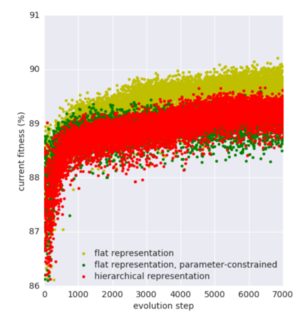
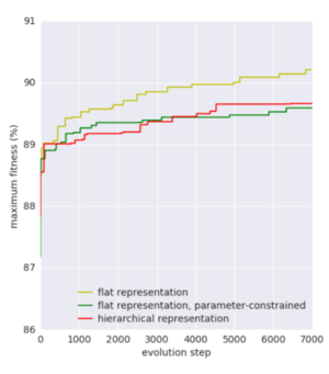
Figure 4 presents the maximum fitness reached by any cell seen by the search framework between each one of the three types of cells, the fitness at time step 200 is, therefore, equivalent to the best model obtained by a random search over 200 architectures from each type of cell.

The total number of parameters used by each genotype at any given time step is shown in Figure 5. It suggests that flat representations tend to add more connections over time and most likely those connections correspond to convolutional operations which in turn require more parameters than other primitive operations.

To run each time step (either initialization or evolutionary) in the search framework, it takes one hour for a GPU to perform four training and evaluation rounds for every single candidate. Therefore, the authors used 200 GPUs simultaneously to complete 7000-time steps in 35 hours. Considering the three types of cell (hierarchical, flat, and parameter-constrained flat), approximately 20000 GPU-hours could be required to replicate the experiment.

Architecture evaluation on CIFAR-10 and ImageNet

Once the evolutionary search finds the best-fitted cells those are plug into the two larger host models to evaluate their performance in those more complex architectures. The first large model (Figure 6) is targeted to image classification on the CIFAR-10 dataset and the second model (Figure 7) is focused on image classification on the ImageNet dataset. Although all the parameters in these two larger host models are trained from scratch including those within the cells, no changes in the cell’s architectures will happen since their structure was found to be optimal during the evolutionary search.

The large CIFAR-10 model is trained with stochastic gradient descent during 80K training steps and decreasing learning rate. To account for the non-negligible standard deviation found when evaluating the exact same model, the percentage of error is determined as the average of five training-evaluation runs.

The ImageNet model is trained with stochastic gradient descent during 200K training steps and decreasing learning rate. For this model, neither standard deviation nor multiple training-evaluation runs were reported.

In section 4.2 three types of cells were described: hierarchical, flat, and parameter-constrained flat. For the hierarchical type of cells, the percentage of error in both large models is reported in Table 1 for four different cases: a cell with random architecture, the best-fitted cell from 200 random architectures, the best-fitted cell from 7000 random architectures, and the best-fitted cell after 7000 evolutionary steps. On the other hand, for the flat and parameter-constrained flat types of architecture, only some of the mentioned four cases are reported in Table 1.

Table 1. Comparison between types of cells and searching method

According to the results in Table 1, for both large host models, the hierarchical cell found by the evolutionary search algorithm achieved the lowest errors with 3.75% in CIFAR-10, 20.3% top-1 error and 5.2% top-5 error in ImageNet. The errors reported in both datasets are calculated by using the trained large models on test sets of images never seen before during any of the previous stages. Even though the cell that follows a hierarchical representation achieved the lowest error, the ones showing the lowest standard deviations are those following a flat representation.

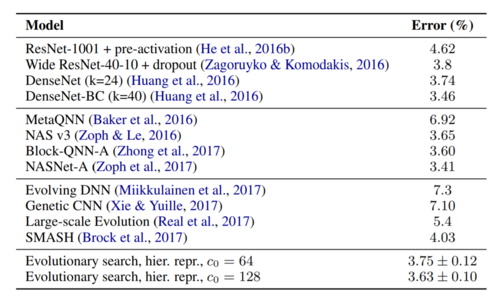
The performance achieved by the large CIFAR-10 host model using the best cell is then compared against other classifiers in Table 2. As an additional improvement, the authors increased the number of channels in its first convolutional layer from 64 to 128. It is worth to note that this first convolutional layer is not part of the cell obtained during the evolutionary search process, instead, it is part of the original host model. The results are grouped into three categories depending on how the classifiers involved in the comparison were created, from top to bottom: handcrafted, reinforcement learning, and evolutionary algorithms.

Table 2. Comparison against other classifiers on CIFAR-10

The classification error achieved by the ImageNet host model when using the best cell is also compared against some high performing image classifiers in the literature and the results are presented in Table 3. Although the classification error scored by the architecture introduced in this paper is not significantly lower than those obtained by state of the art classifiers, it shows outstanding results considering that it is not a hand engineered structure.

Table 3. Comparison against other classifiers on ImageNet

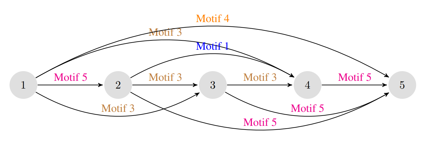
A visualization of the evolved hierarchical cell is shown below. The detailed visualizations of each motif can be seen in Appendix A of the paper. It can be noted that motif 4 directly links the input and output, and itself contains (among other operations) an identity mapping from input to output. Many other such 'skip connections' can be seen.

Conclusion

A new evolutionary framework is introduced for searching neural network architectures over searching spaces defined by flat and hierarchical representations of a convolutional cell, which uses smaller operations instead of the larger ones as the building blocks. The proposed method can achieve strong results with a well-designed architecture even by using simple algorithms such as evolution or random search. Furthermore, experiments show that the proposed framework achieves competitive results against state of the art classifiers on the CIFAR-10 and ImageNet datasets.

Also, compared to contemporary RL-based architecture search approaches, the proposed approach is generally faster with comparable performance.

Critique

While the method introduced in this paper achieves a lower error in comparison to other evolutionary methods, it is not significantly better than those obtained by handcrafted design or reinforcement learning. A more in-depth analysis considering the number of parameters and required computational resources would be necessary to accurately compare the listed methods. I believe they could have described more about the advantages over reinforcement learning.

The paper does not provide enough reasons why the author chose specific two searching algorithms. Possibly more efficient searching is available, which can lead to better performance. Especially, when the performance of the algorithm is not significantly better than previous handcrafted ones, this can be a possible technical improvement.

In section 4.3 it is not clear why the results for the four different cases that are reported for the hierarchical cells in Table 1 are not reported for the ones following a flat representation, considering that the flat cells showed a better performance during the evolutionary search. Recall that the four cases are: a cell with random architecture, the best-fitted cell from 200 random architectures, the best-fitted cell from 7000 random architectures, and the best-fitted cell after 7000 evolutionary steps.

It seems contradictory that the flat type of cells who clearly performed better than the hierarchical ones during the architecture search (section 4.2) are not the ones scoring the lowest error when evaluated on the two large host models (section 4.3).

References

Hanxiao Liu, Karen Simonyan, Oriol Vinyals, Chrisantha Fernando, Koray Kavukcuoglu, https://arxiv.org/abs/1711.00436.

Hierarchical Representations for Efficient Architecture Search

Contents