DON'T DECAY THE LEARNING RATE , INCREASE THE BATCH SIZE
Summary of the ICLR 2018 paper: Don't Decay the learning Rate, Increase the Batch Size
Link: [1]
Summarized by: Afify, Ahmed [ID: 20700841]
INTUITION
Nowadays, it is a common practice not to have a singular steady learning rate for the learning phase of neural network models. Instead, we use adaptive learning rates with the standard gradient descent method. The intuition behind this is that when we are far away from the minima, it is beneficial for us to take large steps towards the minima, as it would require a lesser number of steps to converge, but as we approach the minima, our step size should decrease, otherwise we may just keep oscillating around the minima. In practice, this is generally achieved by methods like SGD with momentum, Nesterov momentum, and Adam. However, the core claim of this paper is that the same effect can be achieved by increasing the batch size during the gradient descent process while keeping the learning rate constant throughout. In addition, the paper argues that such an approach also reduces the parameter updates required to reach the minima, thus leading to greater parallelism and shorter training times. The authors present conclusive experimental evidence to prove the empirical benefits of decaying learning rate can be achieved by increasing the batch size instead.
INTRODUCTION
Stochastic gradient descent (SGD) is the most widely used optimization technique for training deep learning models. The reason for this is that the minima found using this process generalizes well to unseen data (Zhang et al., 2016; Wilson et al., 2017). However, the optimization process is slow and time-consuming as each parameter update corresponds to a small step towards the goal. According to (Goyal et al., 2017; Hoffer et al., 2017; You et al., 2017a), this has motivated researchers to try to speed up this optimization process by taking bigger steps, and hence reduce the number of parameter updates in training a model. This can be achieved by using large batch training, which can be divided across many machines.
However, increasing the batch size leads to decreasing the test set accuracy (Keskar et al., 2016; Goyal et al., 2017). Smith and Le (2017) believed that SGD has a scale of random fluctuations [math]\displaystyle{ g = \epsilon (\frac{N}{B}-1) }[/math], where [math]\displaystyle{ \epsilon }[/math] is the learning rate, [math]\displaystyle{ N }[/math] is the number of training samples, and [math]\displaystyle{ B }[/math] is the batch size. They concluded that there is an optimal batch size proportional to the learning rate when [math]\displaystyle{ B \ll N }[/math], and optimum fluctuation scale [math]\displaystyle{ g }[/math] at constant learning rate which maximizes test set accuracy. This was observed empirically by Goyal et al., 2017 and used to train a ResNet-50 in under an hour with 76.3% validation accuracy on ImageNet dataset.
In this paper, the authors' main goal is to provide evidence that increasing the batch size is quantitatively equivalent to decreasing the learning rate. They show that this approach achieves almost equivalent model performance on the test set with the same number of training epochs but with a remarkably fewer number of parameter updates. The strategy of increasing the batch size during training is in effect decreasing the scale of random fluctuations. Moreover, an additional reduction in the number of parameter updates can be attained by increasing the learning rate and scaling [math]\displaystyle{ B \propto \epsilon }[/math] or even more reduction by increasing the momentum coefficient, [math]\displaystyle{ m }[/math], and scaling [math]\displaystyle{ B \propto \frac{1}{1-m} }[/math]. Although the latter decreases the test accuracy. This has been demonstrated by several experiments on the ImageNet and CIFAR-10 datasets using ResNet-50 and Inception-ResNet-V2 architectures respectively. The authors train ResNet-50 on ImageNet to 76.1% validation accuracy in under 30 minutes.
STOCHASTIC GRADIENT DESCENT AND CONVEX OPTIMIZATION
As mentioned in the previous section, the drawback of SGD when compared to full-batch training is the noise that it introduces that hinders optimization. According to (Robbins & Monro, 1951), there are two equations that govern how to reach the minimum of a convex function: ([math]\displaystyle{ \epsilon_i }[/math] denotes the learning rate at the [math]\displaystyle{ i^{th} }[/math] gradient update)
[math]\displaystyle{ \sum_{i=1}^{\infty} \epsilon_i = \infty }[/math]. This equation guarantees that we will reach the minimum.
[math]\displaystyle{ \sum_{i=1}^{\infty} \epsilon^2_i \lt \infty }[/math]. This equation, which is valid only for a fixed batch size, guarantees that learning rate decays fast enough allowing us to reach the minimum rather than bouncing due to noise.
These equations indicate that the learning rate must decay during training, and second equation is only available when the batch size is constant. To change the batch size, Smith and Le (2017) proposed to interpret SGD as integrating this stochastic differential equation [math]\displaystyle{ \frac{dw}{dt} = -\frac{dC}{dw} + \eta(t) }[/math], where [math]\displaystyle{ C }[/math] represents cost function, [math]\displaystyle{ w }[/math] represents the parameters, and [math]\displaystyle{ \eta }[/math] represents the Gaussian random noise. Furthermore, they proved that noise scale [math]\displaystyle{ g }[/math] controls the magnitude of random fluctuations in the training dynamics by this formula: [math]\displaystyle{ g = \epsilon (\frac{N}{B}-1) }[/math], where [math]\displaystyle{ \epsilon }[/math] is the learning rate, N is the training set size and [math]\displaystyle{ B }[/math] is the batch size. As we usually have [math]\displaystyle{ B \ll N }[/math], we can define [math]\displaystyle{ g \approx \epsilon \frac{N}{B} }[/math]. This explains why when the learning rate decreases, noise [math]\displaystyle{ g }[/math] decreases, enabling us to converge to the minimum of the cost function. However, increasing the batch size has the same effect and makes [math]\displaystyle{ g }[/math] decays with constant learning rate. In this work, the batch size is increased until [math]\displaystyle{ B \approx \frac{N}{10} }[/math], then the conventional way of decaying the learning rate is followed.
SIMULATED ANNEALING AND THE GENERALIZATION GAP
Simulated Annealing: Decaying learning rates are empirically successful. To understand this, they note that introducing random fluctuations whose scale falls during training is also a well-established technique in non-convex optimization; simulated annealing. The initial noisy optimization phase allows exploring a larger fraction of the parameter space without becoming trapped in local minima. Once a promising region of parameter space is located, the noise is reduced to fine-tune the parameters.
Simulated Annealing is a famous technique in non-convex optimization. Starting with the noise in the training process helps us to explore a wide range of parameters. Once we are near the optimum value, noise is reduced to fine tune our final parameters. Nowadays, researchers typically use sharp decay schedules like cosine decay or step-function drops. In physical sciences, slowly annealing (or decaying) the temperature (which is the noise scale in this situation) helps to converge to the global minimum, which is sharp. But decaying the temperature in discrete steps can make the system stuck in a local minimum, which leads to higher cost and lower curvature. The authors think that deep learning has the same intuition. Note that this interpretation may explain why conventional learning rate decay schedules like square roots or exponential decay have become less popular in deep learning in recent years. Increasingly, researchers favor sharper decay schedules like cosine decay or step-function drops. To interpret this shift, we note that it is well known in the physical sciences that slowly annealing the temperature (noise scale) helps the system to converge to the global minimum, which may be sharp.
Generalization Gap: Small batch data generalizes better to the test set than large batch data. Smith and Le (2017) found that there is an optimal batch size which corresponds to optimal noise scale [math]\displaystyle{ g }[/math] [math]\displaystyle{ (g \approx \epsilon \frac{N}{B}) }[/math]. They found an optimum batch size [math]\displaystyle{ B_{opt} \propto \epsilon N }[/math] that maximizes test set accuracies. This means that gradient noise is helpful as it makes SGD escape sharp minima which do not generalize well.
THE EFFECTIVE LEARNING RATE AND THE ACCUMULATION VARIABLE
The Effective Learning Rate : [math]\displaystyle{ \epsilon_{eff} = \frac{\epsilon}{1-m} }[/math]
Smith and Le (2017) included momentum [math]\displaystyle{ m }[/math] to the vanilla SGD noise scale equation, [math]\displaystyle{ g = \frac{\epsilon}{1-m}(\frac{N}{B}-1)\approx \frac{\epsilon N}{B(1-m)} }[/math]. They found that by increasing the learning rate and the momentum while proportionally scaling [math]\displaystyle{ B \propto \frac{\epsilon }{1-m} }[/math], further reduces the number of parameter updates needed during training. However, test accuracy decreases when the momentum coefficient is increased.
To understand the reasons behind this, we need to analyze momentum update equations below:
[math]\displaystyle{ \Delta w = -A\epsilon }[/math]
We can see that the accumulation variable [math]\displaystyle{ A }[/math], starting at 0, increases exponentially until it reaches its steady state value during [math]\displaystyle{ \frac{B}{N(1-m)} }[/math] training epochs. If [math]\displaystyle{ \Delta w }[/math] is suppressed, it can reduce the rate of convergence.
Moreover, at high momentum, we have four challenges:
- Additional epochs are needed to catch up with the accumulation.
- Accumulation needs more time [math]\displaystyle{ \frac{B}{N(1-m)} }[/math] to forget old gradients.
- After this time, however, the accumulation cannot adapt to changes in the loss landscape.
- In the early stage, a large batch size will lead to the instabilities.
It is thus recommended to keep a reduced learning rate for the first few epochs of training.
EXPERIMENTS
SIMULATED ANNEALING IN A WIDE RESNET
Dataset: CIFAR-10 (50,000 training images)
Network Architecture: “16-4” wide ResNet
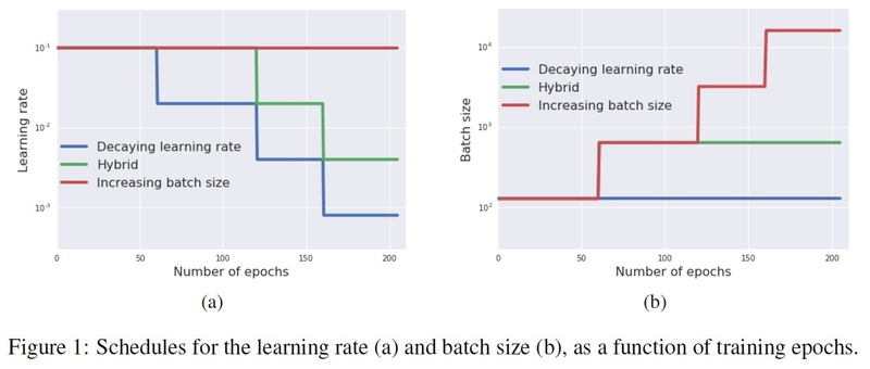
Training Schedules used as in the below figure: . These demonstrate the equivalence between decreasing the learning rate and increasing the batch size.
- Decaying learning rate: learning rate decays by a factor of 5 at a sequence of “steps”, and the batch size is constant
- Increasing batch size: learning rate is constant, and the batch size is increased by a factor of 5 at every step.
- Hybrid: At the beginning, the learning rate is constant and batch size is increased by a factor of 5. Then, the learning rate decays by a factor of 5 at each subsequent step, and the batch size is constant. This is the schedule that will be used if there is a hardware limit affecting a maximum batch size limit.
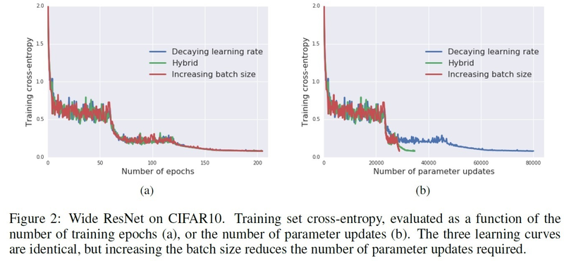
If the learning rate itself must decay during training, then these schedules should show different learning curves (as a function of the number of training epochs) and reach different final test set accuracies. Meanwhile, if it is the noise scale which should decay, all three schedules should be indistinguishable.
As shown in the below figure: in the left figure (2a), we can observe that for the training set, the three learning curves are exactly the same while in figure 2b, increasing the batch size has a huge advantage of reducing the number of parameter updates. This concludes that noise scale is the one that needs to be decayed and not the learning rate itself
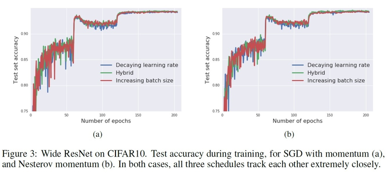
To make sure that these results are the same for the test set as well, in figure 3, we can see that the three learning curves are exactly the same for SGD with momentum, and Nesterov momentum. In figure 3b, the test set accuracy when training with Nesterov momentum parameter 0.9 is presented.
To check for other optimizers as well. the below figure shows the same experiment as in figure 3, which is the three learning curves for the test set, but for vanilla SGD and Adam, and showing
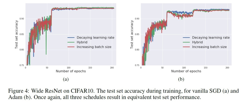
In figure 4a, the same experiment is repeated with vanilla SGD, again obtaining three similar curves. Finally, in figure 4b, the authors repeat the experiment with Adam. They also use the default parameter settings of TensorFlow, such that the initial base learning rate here is 0.01, β1 = 0.9 and β2 = 0.999.
Conclusion: Decreasing the learning rate and increasing the batch size during training are equivalent
INCREASING THE EFFECTIVE LEARNING RATE
Here, the focus is on minimizing the number of parameter updates required to train a model. As shown above, the first step is to replace decaying learning rates by increasing batch sizes. Now, the authors show here that we can also increase the effective learning rate [math]\displaystyle{ \epsilon_{eff} = \epsilon/(1 − m) }[/math] at the start of training, while scaling the initial batch size [math]\displaystyle{ B \propto \epsilon_{eff} }[/math] . All experiments are conducted using SGD with momentum. There are 50000 images in the CIFAR-10 training set, and since the scaling rules only hold when [math]\displaystyle{ B \lt \lt N }[/math] , we decided to set a maximum batch size [math]\displaystyle{ B_{max} }[/math]= 5120 .
Dataset: CIFAR-10 (50,000 training images)
Network Architecture: “16-4” wide ResNet
Training Parameters: Optimization Algorithm: SGD with momentum / Maximum batch size = 5120
Training Schedules:
The authors consider four training schedules, all of which decay the noise scale by a factor of five in a series of three steps with the same number of epochs.
Original training schedule: initial learning rate of 0.1 which decays by a factor of 5 at each step, a momentum coefficient of 0.9, and a batch size of 128. Follows the implementation of Zagoruyko & Komodakis (2016).
Increasing batch size: learning rate of 0.1, momentum coefficient of 0.9, initial batch size of 128 that increases by a factor of 5 at each step.
Increased initial learning rate: initial learning rate of 0.5, initial batch size of 640 that increase during training.
Increased momentum coefficient: increased initial learning rate of 0.5, initial batch size of 3200 that increase during training, and an increased momentum coefficient of 0.98.
The results of all training schedules, which are presented in the below figure, are documented in the following table:

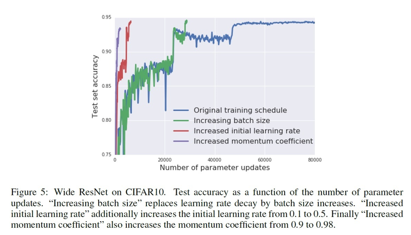
Conclusion: Increasing the effective learning rate and scaling the batch size results in further reduction in the number of parameter updates
TRAINING IMAGENET IN 2500 PARAMETER UPDATES
A) Experiment Goal: Control Batch Size
Dataset: ImageNet (1.28 million training images)
The paper modified the setup of Goyal et al. (2017), and used the following configuration:
Network Architecture: Inception-ResNet-V2
Training Parameters:
90 epochs / noise decayed at epoch 30, 60, and 80 by a factor of 10 / Initial ghost batch size = 32 / Learning rate = 3 / momentum coefficient = 0.9 / Initial batch size = 8192
Two training schedules were used:
“Decaying learning rate”, where batch size is fixed and the learning rate is decayed
“Increasing batch size”, where batch size is increased to 81920 then the learning rate is decayed at two steps.

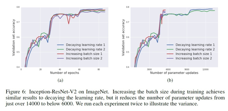
Conclusion: Increasing the batch size resulted in reducing the number of parameter updates from 14,000 to 6,000.
B) Experiment Goal: Control Batch Size and Momentum Coefficient
Training Parameters: Ghost batch size = 64 / noise decayed at epoch 30, 60, and 80 by a factor of 10.
The below table shows the number of parameter updates and accuracy for different sets of training parameters:

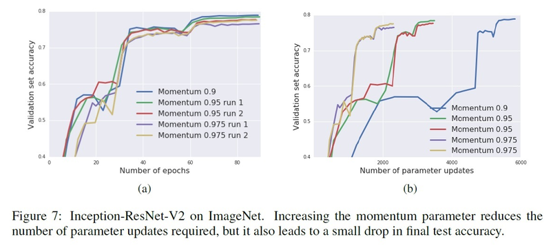
Conclusion: Increasing the momentum reduces the number of parameter updates but leads to a drop in the test accuracy.
TRAINING IMAGENET IN 30 MINUTES
Dataset: ImageNet (already introduced in the previous section)
Network Architecture: ResNet-50
The paper replicated the setup of Goyal et al. (2017) while modifying the number of TPU devices, batch size, learning rate, and then calculating the time to complete 90 epochs, and measuring the accuracy, and performed the following experiments below:

Conclusion: Model training times can be reduced by increasing the batch size during training.
RELATED WORK
Main related work mentioned in the paper is as follows:
- Smith & Le (2017) interpreted Stochastic gradient descent as a stochastic differential equation; the paper built on this idea to include decaying learning rate.
- Mandt et al. (2017) analyzed how to modify SGD for the task of Bayesian posterior sampling.
- Keskar et al. (2016) focused on the analysis of noise once the training is started.
- Moreover, the proportional relationship between batch size and learning rate was first discovered by Goyal et al. (2017) and successfully trained ResNet-50 on ImageNet in one hour after discovering the proportionality relationship between batch size and learning rate.
- Furthermore, You et al. (2017a) presented Layer-wise Adaptive Rate Scaling (LARS), which is applying different learning rates to train ImageNet in 14 minutes and 74.9% accuracy.
- Wilson et al. (2017) argued that adaptive optimization methods tend to generalize less well than SGD and SGD with momentum (although they did not include K-FAC in their study), while the authors' work reduces the gap in convergence speed.
- Finally, another strategy called Asynchronous-SGD that allowed (Recht et al., 2011; Dean et al., 2012) to use multiple GPUs even with small batch sizes.
CONCLUSIONS
Increasing the batch size during training has the same benefits of decaying the learning rate in addition to reducing the number of parameter updates, which corresponds to faster training time. Experiments were performed on different image datasets and various optimizers with different training schedules to prove this result. The paper proposed to increase the learning rate and momentum parameter [math]\displaystyle{ m }[/math], while scaling [math]\displaystyle{ B \propto \frac{\epsilon}{1-m} }[/math], which achieves fewer parameter updates, but slightly less test set accuracy as mentioned in detail in the experiments’ section. In summary, on ImageNet dataset, Inception-ResNet-V2 achieved 77% validation accuracy in under 2500 parameter updates, and ResNet-50 achieved 76.1% validation set accuracy on TPU in less than 30 minutes. One of the great findings of this paper is that all the methods use the hyper-parameters directly from previous works in the literature, and no additional hyper-parameter tuning was performed.
CRITIQUE
Pros:
- The paper showed empirically that increasing batch size and decaying learning rate are equivalent.
- Several experiments were performed on different optimizers such as SGD and Adam.
- Had several comparisons with previous experimental setups.
- The authors provide quantitative evaluations of their hypothesis by replicating the original training process previously published by other researchers and also implementing an additional training process with an increased batch size. This paper shows the importance of giving enough details not only about the algorithms but also about the hyperparameters, hardware, and other training details that can help other researchers explore other ideas.
Cons:
- All datasets used are image datasets. Other experiments should have been done on datasets from different domains to ensure generalization.
- The number of parameter updates was used as a comparison criterion, but wall-clock times could have provided additional measurable judgment although they depend on the hardware used.
- Special hardware is needed for large batch training, which is not always feasible. As batch-size increases, we generally need more RAM to train the same model. However, if the learning rate is decreased, the RAM use remains constant. As a result, learning rate decay will allow us to train bigger models.
- In section 5.2 (Increasing the Effective Learning rate), the authors did not test a range of learning rate values and used only (0.1 and 0.5). Additional results from varying the initial learning rate values from 0.1 to 3.2 are provided in the appendix, which indicates that the test accuracy begins to fall for initial learning rates greater than ~0.4. The appended results do not show validation set accuracy curves like in Figure 6, however. It would be beneficial to see if they were similar to the original 0.1 and 0.5 initial learning rate baselines.
- Although the main idea of the paper is interesting, its results do not seem to be too surprising in comparison with other recent papers in the subject.
- The paper could benefit from using some other models to demonstrate its claim and generalize its idea by adding some comparisons with other models as well as other recent methods to increase batch size.
- The paper presents interesting ideas. However, it lacks mathematical and theoretical analysis beyond the idea. Since the experiment is primary on image dataset and it does not provide sufficient theories, the paper itself presents limited applicability to other types.
- Also, in an experimental setting, only single training runs from one random initialization is used. It would be better to take the best of many runs or to show confidence intervals.
- It is proposed that we should compare learning rate decay with batch-size increase under the setting that total budget/number of training samples is fixed.
- While the paper demonstrated the proposed solution can decrease training time, it is not an entirely fair comparison because computations were distributed on a TPU POD. Suppose computing resource remains the same, the purposed method may possibly train slower.
REFERENCES
- Takuya Akiba, Shuji Suzuki, and Keisuke Fukuda. Extremely large minibatch sgd: Training resnet-50 on imagenet in 15 minutes. arXiv preprint arXiv:1711.04325, 2017.
- Lukas Balles, Javier Romero, and Philipp Hennig. Coupling adaptive batch sizes with learning rates.arXiv preprint arXiv:1612.05086, 2016.
- L´eon Bottou, Frank E Curtis, and Jorge Nocedal. Optimization methods for large-scale machine learning.arXiv preprint arXiv:1606.04838, 2016.
- Richard H Byrd, Gillian M Chin, Jorge Nocedal, and Yuchen Wu. Sample size selection in optimization methods for machine learning. Mathematical programming, 134(1):127–155, 2012.
- Pratik Chaudhari, Anna Choromanska, Stefano Soatto, and Yann LeCun. Entropy-SGD: Biasing gradient descent into wide valleys. arXiv preprint arXiv:1611.01838, 2016.
- Soham De, Abhay Yadav, David Jacobs, and Tom Goldstein. Automated inference with adaptive batches. In Artificial Intelligence and Statistics, pp. 1504–1513, 2017.
- Jeffrey Dean, Greg Corrado, Rajat Monga, Kai Chen, Matthieu Devin, Mark Mao, Andrew Senior, Paul Tucker, Ke Yang, Quoc V Le, et al. Large scale distributed deep networks. In Advances in neural information processing systems, pp. 1223–1231, 2012.
- Michael P Friedlander and Mark Schmidt. Hybrid deterministic-stochastic methods for data fitting.SIAM Journal on Scientific Computing, 34(3):A1380–A1405, 2012.
- Priya Goyal, Piotr Doll´ar, Ross Girshick, Pieter Noordhuis, Lukasz Wesolowski, Aapo Kyrola, Andrew Tulloch, Yangqing Jia, and Kaiming He. Accurate, large minibatch SGD: Training imagenet in 1 hour. arXiv preprint arXiv:1706.02677, 2017.
- Sepp Hochreiter and J¨urgen Schmidhuber. Flat minima. Neural Computation, 9(1):1–42, 1997.
- Elad Hoffer, Itay Hubara, and Daniel Soudry. Train longer, generalize better: closing the generalization gap in large batch training of neural networks. arXiv preprint arXiv:1705.08741, 2017.
- Norman P Jouppi, Cliff Young, Nishant Patil, David Patterson, Gaurav Agrawal, Raminder Bajwa, Sarah Bates, Suresh Bhatia, Nan Boden, Al Borchers, et al. In-datacenter performance analysis of a tensor processing unit. In Proceedings of the 44th Annual International Symposium on Computer Architecture, pp. 1–12. ACM, 2017.
- Nitish Shirish Keskar, Dheevatsa Mudigere, Jorge Nocedal, Mikhail Smelyanskiy, and Ping Tak Peter Tang. On large-batch training for deep learning: Generalization gap and sharp minima. arXiv preprint arXiv:1609.04836, 2016.
- Diederik Kingma and Jimmy Ba. Adam: A method for stochastic optimization. arXiv preprint arXiv:1412.6980, 2014.
- Alex Krizhevsky. One weird trick for parallelizing convolutional neural networks. arXiv preprint arXiv:1404.5997, 2014.
- Qianxiao Li, Cheng Tai, and E Weinan. Stochastic modified equations and adaptive stochastic gradient algorithms. arXiv preprint arXiv:1511.06251, 2017.
- Ilya Loshchilov and Frank Hutter. SGDR: stochastic gradient descent with restarts. arXiv preprint arXiv:1608.03983, 2016.
- Stephan Mandt, Matthew D Hoffman, and DavidMBlei. Stochastic gradient descent as approximate bayesian inference. arXiv preprint arXiv:1704.04289, 2017.
- James Martens and Roger Grosse. Optimizing neural networks with kronecker-factored approximate curvature. In International Conference on Machine Learning, pp. 2408–2417, 2015.
- Yurii Nesterov. A method of solving a convex programming problem with convergence rate o (1/k2). In Soviet Mathematics Doklady, volume 27, pp. 372–376, 1983.
- Lutz Prechelt. Early stopping-but when? Neural Networks: Tricks of the trade, pp. 553–553, 1998.
- Benjamin Recht, Christopher Re, Stephen Wright, and Feng Niu. Hogwild: A lock-free approach to parallelizing stochastic gradient descent. In Advances in neural information processing systems, pp. 693–701, 2011.
- Herbert Robbins and Sutton Monro. A stochastic approximation method. The annals of mathematical statistics, pp. 400–407, 1951.
- Samuel L. Smith and Quoc V. Le. A bayesian perspective on generalization and stochastic gradient descent. arXiv preprint arXiv:1710.06451, 2017.
- Christian Szegedy, Sergey Ioffe, Vincent Vanhoucke, and Alexander A Alemi. Inception-v4, Inception-ResNet and the impact of residual connections on learning. In AAAI, pp. 4278–4284, 2017.
- Max Welling and Yee W Teh. Bayesian learning via stochastic gradient langevin dynamics. In Proceedings of the 28th International Conference on Machine Learning (ICML-11), pp. 681–688, 2011.
- Ashia C Wilson, Rebecca Roelofs, Mitchell Stern, Nathan Srebro, and Benjamin Recht. The marginal value of adaptive gradient methods in machine learning. arXiv preprint arXiv:1705.08292, 2017.
- Yang You, Igor Gitman, and Boris Ginsburg. Scaling SGD batch size to 32k for imagenet training. arXiv preprint arXiv:1708.03888, 2017a.
- Yang You, Zhao Zhang, C Hsieh, James Demmel, and Kurt Keutzer. Imagenet training in minutes. CoRR, abs/1709.05011, 2017b.
- Sergey Zagoruyko and Nikos Komodakis. Wide residual networks. arXiv preprint arXiv:1605.07146, 2016.
- Chiyuan Zhang, Samy Bengio, Moritz Hardt, Benjamin Recht, and Oriol Vinyals. Understanding deep learning requires rethinking generalization. arXiv preprint arXiv:1611.03530, 2016.