DETECTING STATISTICAL INTERACTIONS FROM NEURAL NETWORK WEIGHTS: Difference between revisions
No edit summary |
m (Kb7lee moved page User:Kb7lee to statwiki:DETECTING STATISTICAL INTERACTIONS FROM NEURAL NETWORK WEIGHTS) |
(No difference)
| |
Revision as of 02:27, 26 November 2018
Introduction
Within several areas, regression analysis is essential. However, due to complexity, the only tool left for practitioners are some simple tools based on linear regression. Growth in computational power available, practitioners are now able to use complicated models. Nevertheless, now the problem is not complexity: Interpretability. Neural network mostly exhibits superior predictable power compare to other traditional statistical regression methods. However, it's highly complicated structure simply prevent users to understand the results. In this paper, we are going to present one way of implementing interpretability in neural network.
Note that in this paper, we only consider one specific types of neural network, Feed-Forward Neural Network. Based on the methodology discussed here, we can build interpretation methodology for other types of networks also.
Notations
Before we dive in to methodology, we are going to define a few notations here. Most of them will be trivial.
1. Vector: Vectors are defined with bold-lowercases, v, w
2. Matrix: Matrice are defined with blod-uppercases, V, W
3. Interger Set: For some interger p [math]\displaystyle{ \in }[/math] Z, we define [p] := {1,2,3,...,p}
Interaction
First of all, in order to explain the model, we need to be able to explain the interactions and their effects to output. Therefore, we define 'interacion' between variables as below.

From the definition above, for a function like, [math]\displaystyle{ x_1x_2 + sin(x_3 + x_4 + x_5) }[/math], we have [math]\displaystyle{ {[x_1, x_2]} }[/math] and [math]\displaystyle{ {[x_3, x_4, x_5]} }[/math] interactions. And we say that the latter interaction to be 3-way interaction.
Note that from the definition above, we can naturally deduce that d-way interaction can exist if and only if all of its (d-1) interactions exist. For example, 3-way interaction above shows that we have 2-way interactions [math]\displaystyle{ {[3,4], [4,5]} }[/math] and [math]\displaystyle{ {[3,5]} }[/math].
One thing that we need to keep in mind is that for models like neural network, most of interactions are happening within hidden layers. This means that we needa proper way of measuring interaction strength.
The key observation is that for any kinds of interaction, at a some hidden unit of some hidden layer, two interacting features the ancestors. In graph-theoretical language, interaction map can be viewed as an associated directed graph and for any interaction [math]\displaystyle{ \Gamma \in [p] }[/math], there exists at least one vertix that has all of features of [math]\displaystyle{ \Gamma }[/math] as ancestors. The statement can be rigorized as the following:

Now, the above mathematical statement gurantees us to measure interaction strengths at ANY hidden layers. For example, if we want to study about interactions at some specific hidden layer, now we now that there exists corresponding vertices between the hidden layer and output layer. Therefore all we need to do is now to find approprite measure which can summarize the information between those two layers. } Before doing so, let's think about a single-layered neural network. For any one hidden unit, we can have possibly, [math]\displaystyle{ 2^{||W_i,:||} }[/math], number of interactions. This means that our search space might be too huge for multi-layered networks. Therefore, we need a some descent way of approximate out search space.
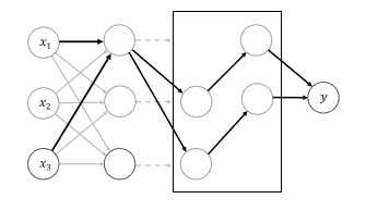
As we discussed above, in order to consider interaction between units in any layers, we need to think about their out-going paths. However, we soon encountered the fact that for some fully-connected multi-layer neural network, the search space might be too huge to compare. Therefore, we use information about out-going paths gredient upper bond. To represent the influence of out-going paths at [math]\displaystyle{ l }[/math]-hidden layer, we define cumulative impact of weights between output layer and [math]\displaystyle{ l+1 }[/math]. We define aggregated weights as,

Note that [math]\displaystyle{ z^{(l)} \in R^{(p_l)} }[/math] where [math]\displaystyle{ p_l }[/math] is the number of hidden units in [math]\displaystyle{ l }[/math]-layer.
Moreover, this is the lipschitz constant of gredients. Gredient has been an import variable of measuring influence of features, especially when we consider that input layer's derivative computes the direction normal to decision boundaries.
Quantifying influence
For some [math]\displaystyle{ i }[/math] hidden unit at the first hidden layer, which is the closet layer to the input layer, we define the influence strength of some interaction as,

The function [math]\displaystyle{ \mu }[/math] will be defined later. Essentially, the formula shows that the strength of influence is defined as the product of the aggregated weight on the first hidden layer and some measure of influence between the first hidden layer and the input layer.
For the function, [math]\displaystyle{ \mu }[/math], any positive-real valued functions such as max, min and average can be candidates. The effects of those candidates will be tested later.
Now based on the specifications above, the author suggested the algorithm for searching influential interactions between input layer units as follows:

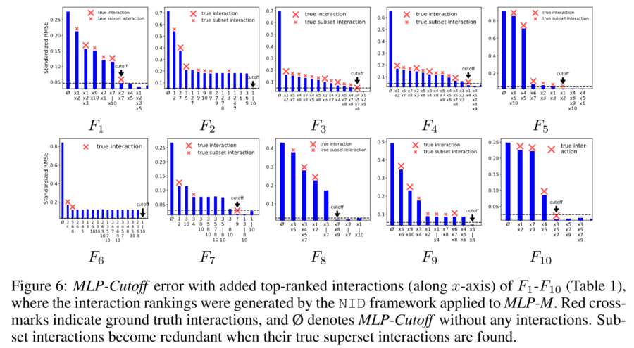
Cut off Model
Now using the greedy algorithm defined above, we can rank the interactions by their strength. However, in order to access true interactions, we are building the cut off model which is a generalized additive model (GAM) as below,

From the above model, each [math]\displaystyle{ g }[/math] and [math]\displaystyle{ g^* }[/math] are Feed-Forward neural network. We are keep adding interactions until the performance reaches plateaus.
Experiment
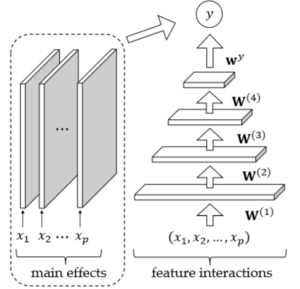
For the experiment, we are going to compare three neural network model with traditional statistical interaction detecting algorithms. For the nueral network models, first model will be MLP, second model will be MLP-M, which is MLP with additional univariate network at the output. The last one is the cut-off model defined above, which is denoted by MLP-cutoff. MLP-M model is graphically represented below.
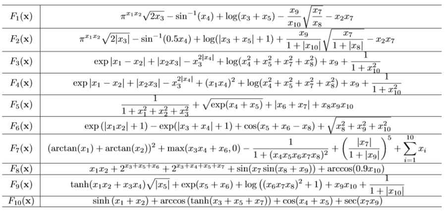
For the experiment, we are going to test on 10 synthetic functions.
And the author also reported the results of comparisons between the models. As you can see, neural network based models are performing better in average. Compare to the traditional methods liek ANOVA, MLP and MLP-M method shows 20% increases in performance.
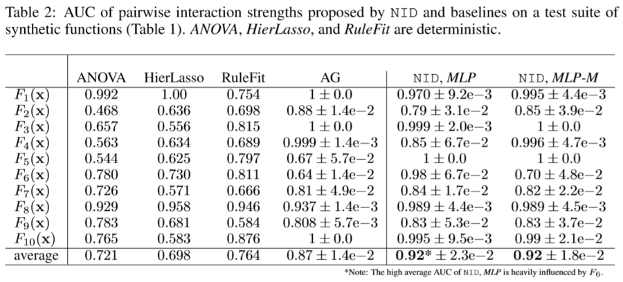
The above result shows that MLP-M almost perfectly catch the most influential pair-wise interactions.
Limitations
Even though for the above synthetic experiment MLP methods showed superior performances, the method still have some limitations. For example, fir the function like, [math]\displaystyle{ x_1x_2 + x_2x_3 + x_1x_3 }[/math], neural network fails to distinguish between interlinked interactions to single higher order interaction. Moreoever, correlation between features deteriorates the ability of the network to distinguish interactions. However, correlation issues are presented most of interaction detection algorithms.
Conclusion
Here we presented the method of detecting interactions using MLP. Compared to other state-of-the-art methods like Additive Groves (AG), the performances are competitive yet computational powers required is far less. Therefore, it is safe to claim that the method will be extremly useful for practitioners with (comparably) less computational powers. Moreover, the NIP algorithm successfully reduced the computation sizes. After all, the most important aspect of this algorithm is that now users of nueral networks can impose interpretability in the model usage, which will change the level of usability to another level for most of practitioners outside of those working in machine learning and deep learning areas.
Reference
[1] Jacob Bien, Jonathan Taylor, and Robert Tibshirani. A lasso for hierarchical interactions. Annals of statistics, 41(3):1111, 2013.
[2] G David Garson. Interpreting neural-network connection weights. AI Expert, 6(4):46–51, 1991.
[3] Yotam Hechtlinger. Interpretation of prediction models using the input gradient. arXiv preprint arXiv:1611.07634, 2016.
[4] Shiyu Liang and R Srikant. Why deep neural networks for function approximation? 2016.
[5] David Rolnick and Max Tegmark. The power of deeper networks for expressing natural functions. International Conference on Learning Representations, 2018.
[6] Daria Sorokina, Rich Caruana, and Mirek Riedewald. Additive groves of regression trees. Machine Learning: ECML 2007, pp. 323–334, 2007.
[7] Simon Wood. Generalized additive models: an introduction with R. CRC press, 2006