DETECTING STATISTICAL INTERACTIONS FROM NEURAL NETWORK WEIGHTS
Introduction
It has been commonly believed that one major advantage of neural networks is their capability of modeling complex statistical interactions between features for automatic feature learning. Statistical interactions capture important information on where features often have joint effects with other features on predicting an outcome. The discovery of interactions is especially useful for scientific discoveries and hypothesis validation. For example, physicists may be interested in understanding what joint factors provide evidence for new elementary particles; doctors may want to know what interactions are accounted for in risk prediction models, to compare against known interactions from existing medical literature.
With the growth in the computational power available Neural Networks have been able to solve many of the complex tasks in a wide variety of fields. This is mainly due to their ability to model complex and non-linear interactions. Neural networks have traditionally been treated as “black box” models, preventing their adoption in many application domains, such as those where explainability is desirable. It has been noted that complex machine learning models can learn unintended patterns from data, raising significant risks to stakeholders [14]. Therefore, in applications where machine learning models are intended for making critical decisions, such as healthcare or finance, it is paramount to understand how they make predictions [9]. Within several areas, like eg: computation social science, interpretability is of utmost importance. Since we do not understand how a neural network comes to its decision, practitioners in these areas tend to prefer simpler models like linear regression, decision trees, etc. which are much more interpretable. In this paper, we are going to present one way of implementing interpretability in a neural network.
Existing approaches to interpreting neural networks can be summarized into two types. One type is direct interpretation, which focuses on 1) explaining individual feature importance, for example by computing input gradients [13] and decomposing predictions [8], 2) developing attention-based models, which illustrate where neural networks focus during inference [11], and 3) providing model-specific visualizations, such as feature map and gate activation visualizations [15]. The other type is indirect interpretation, for example, post-hoc interpretations of feature importance [12] and knowledge distillation to simpler interpretable models [10].
In this paper, the authors propose Neural Interaction Detection (NID), which can detect any order or form of statistical interaction captured by the feedforward neural network by examining its weight matrix. This approach is efficient because it avoids searching over an exponential solution space of interaction candidates by making an approximation of hidden unit importance at the first hidden layer via all weights above and doing a 2D traversal of the input weight matrix.The authors also provide theoretical justifications as to why, interactions between features are created at hidden units and why the hidden unit approximation satisfies bounds on hidden unit gradients. Top -K interactions are determined from interaction rankings by using a special form of generalized additive model, which accounts for interactions of variable order.
Note that in this paper, we only consider one specific types of neural network, feedforward neural network. Based on the methodology discussed here, the authors suggest that we can build an interpretation method for other types of networks also.
Related Work
1. Interaction Detection approaches:
- Conduct individual tests for all features' combination such as ANOVA and Additive Groves. Two-way ANOVA has been a standard method of performing pairwise interaction detection that involves conducting hypothesis tests for each interaction candidate by checking each hypothesis with F-statistics (Wonnacott & Wonnacott, 1972). Additive Groves is another method that conducts individual tests for interactions and hence must face the same computational difficulties; however, it is special because the interactions it detects are not constrained to any functional form.
- Define all interaction forms of interest, then later finds the important ones.
- The paper's goal is to detect interactions without compromising the functional forms. Our method accomplishes higher-order interaction detection, which has the benefit of avoiding a high false positive or false discovery rate.
2. Interpretability: A lot of work has also been done in this particular area and it can be divided it the following broad categories:
- Feature Importance through Decomposition: Methods like Input Gradient(Sundararajan et al., 2017) learns the importance of features through a gradient-based approach similar to backpropagation. Works like Li et al(2017), Murdoch(2017) and Murdoch(2018) study interpretability of LSTMs by looking at phrase and word level importance scores. Bach et al. 2015 and Shrikumar et al. 2016 (DeepLift) study pixel importance in CNNs.
- Studying Visualizations in Models - Karpathy et al. (2015) worked with character generating LSTMs and tried to study activation and firing in certain hidden units for meaningful attributes. (Yosinski et al., 2015 studies feature map visualizations, providing a tool for visualizing live activations on each layer of a trained CNN, and another for visualizing "Regularized Optimization".)
- Attention-Based Models: Bahdanau et al. (2014) - These are a different class of models which use attention modules(different architectures) to help focus the neural network to decide the parts of the input that it should look more closely or give more importance to. Looking at the results of these type of model an indirect sense of interpretability can be gauged.
- Sum product networks, Hoifun Poon, Pedro Domingos (2011) It is a new deep architecture that provides clear semantics. In its core, it is a probabilistic model, with two types of nodes: Sum node and Product nodes. The sum nodes are trying to model the mixture of distributions and product node is trying to model joint distributions. It can be trained using gradient descent and other methods as well. The main advantage of the Sum-Product Network is that it has clear semantics, where people can interpret exactly how the network models make decisions. Therefore, it has better interpretability than most of the current deep architectures.
The approach in this paper is to extract non-additive interactions between variables from the neural network weights.
Notations
Before we dive into methodology, we are going to define a few notations here. Most of them will be trivial.
1. Vector: Vectors are defined with bold-lowercases, v, w
2. Matrix: Matrices are defined with bold-uppercases, V, W
3. Interger Set: For some interger p [math]\displaystyle{ \in }[/math] Z, we define [p] := {1,2,3,...,p}
Interaction
First of all, in order to explain the model, we need to be able to explain the interactions and their effects to output. Therefore, we define 'interaction' between variables as below.

From the definition above, for a function like, [math]\displaystyle{ x_1x_2 + sin(x_3 + x_4 + x_5) }[/math], we have [math]\displaystyle{ {[x_1, x_2]} }[/math] and [math]\displaystyle{ {[x_3, x_4, x_5]} }[/math] interactions. And we say that the latter interaction to be 3-way interaction.
Note that from the definition above, we can naturally deduce that d-way interaction can exist if and only if all of its (d-1) interactions exist. For example, 3-way interaction above shows that we have 2-way interactions [math]\displaystyle{ {[3,4], [4,5]} }[/math] and [math]\displaystyle{ {[3,5]} }[/math].
One thing that we need to keep in mind is that for models like neural networks, most of the interactions are happening within hidden layers. This means that we need a proper way of measuring interaction strength.
The key observation is that for any kinds of interaction, at some hidden unit of some hidden layer, two interacting features the ancestors. In graph-theoretical language, interaction map can be viewed as an associated directed graph and for any interaction [math]\displaystyle{ \Gamma \in [p] }[/math], there exists at least one vertex that has all of the features of [math]\displaystyle{ \Gamma }[/math] as ancestors. The statement can be rigorized as the following:

Now, the above mathematical statement guarantees us to measure interaction strengths at ANY hidden layers. For example, if we want to study interactions at some specific hidden layer, now we now that there exists corresponding vertices between the hidden layer and output layer. Therefore all we need to do is now to find appropriate measure which can summarize the information between those two layers.
Before doing so, let's think about a single-layered neural network. For any single hidden unit, we can have possibly, [math]\displaystyle{ 2^{||W_i,:||} }[/math], number of interactions. This means that our search space might be too huge for multi-layered networks. Therefore, we need some descent way of approximate out search space. Moreover, the authors realized a fast interaction detection by limiting the search complexity of the task by only quantifying interactions created at the first hidden layer. The figure below illustrates an interaction within a fully connected feedforward neural network, where the box contains later layers in the network.
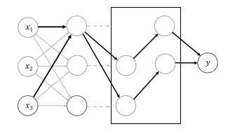
As we discussed above, in order to consider the interaction between units in any layers, we need to think about their out-going paths. However, we soon encountered the fact that for some fully-connected multi-layer neural network, the search space might be too huge to compare. Therefore, we use information about out-going paths gradient upper bond. To represent the influence of out-going paths at [math]\displaystyle{ l }[/math]-hidden layer, we define cumulative impact of weights between output layer and [math]\displaystyle{ l+1 }[/math]. We define aggregated weights as,

Note that [math]\displaystyle{ z^{(l)} \in R^{(p_l)} }[/math] where [math]\displaystyle{ p_l }[/math] is the number of hidden units in [math]\displaystyle{ l }[/math]-layer.
Moreover, this is the lipschitz constant of gradients. Gradient has been an import variable of measuring the influence of features, especially when we consider that input layer's derivative computes the direction normal to decision boundaries. Hence an upper bound on the gradient magnitude approximates how important the variable can be.
Quantifying influence
For some [math]\displaystyle{ i }[/math] hidden unit at the first hidden layer, which is the closet layer to the input layer, we define the influence strength of some interaction as,

The function [math]\displaystyle{ \mu }[/math] will be defined later. Essentially, the formula shows that the strength of influence is defined as the product of the aggregated weight on the first hidden layer and some measure of influence between the first hidden layer and the input layer.
For the function, [math]\displaystyle{ \mu }[/math], any positive-real valued functions such as max, min and average can be candidates. The effects of those candidates will be tested later.
Now based on the specifications above, the author suggested the algorithm for searching influential interactions between input layer units as follows:
It was pointed out that restricting to the first hidden layer might miss some important feature interactions, however, the author state that it is not straightforward how to incorporate the idea of hidden units at intermediate layers to get better interaction detection performance.

Cut-off Model
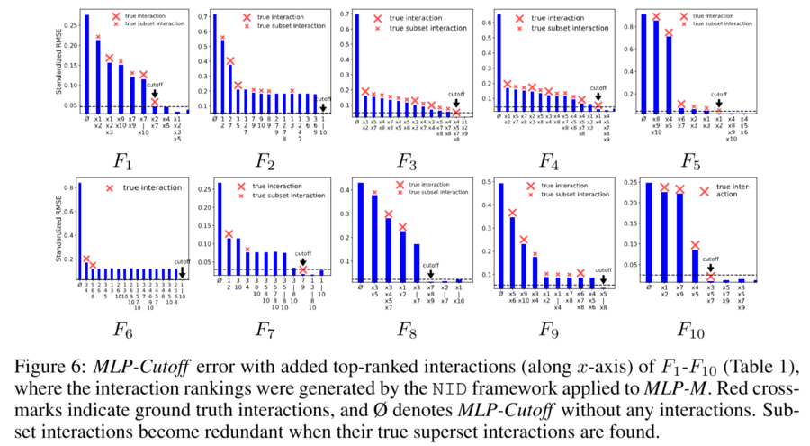
Now using the greedy algorithm defined above, we can rank the interactions by their strength. However, in order to access true interactions, we are building the cut-off model which is a generalized additive model (GAM) as below,
From the above model, each of [math]\displaystyle{ g_i }[/math] and [math]\displaystyle{ g_i' }[/math] are Feed-Forward neural networks. [math]\displaystyle{ g_i(\cdot) }[/math] captures the main effects, while [math]\displaystyle{ g_i'(\cdot) }[/math] captures the interaction. We are keep adding interactions until the performance reaches plateaus.
Pairwise Interaction Detection
A variant to the authors interaction algorithm tests for all pairwise interactions. Modelling pairwise interactions is the de facto objective of many machine learning algorithms such as factorization machines and hierarchical lasso. The authors rank all pairwise features accorind to their strengths denoted by [math]\displaystyle{ w({i,j}) }[/math] , calculated on the first hidden layer, where again the leveraging function is [math]\displaystyle{ min(.) }[/math] and[math]\displaystyle{ w({i,j}) }[/math] = [math]\displaystyle{ \sum_{s=1}^{p_1}w_s({i,j}) }[/math]. The higher the rank calculated by above equations, the more likely the interactions exist.
Experiment
For the experiment, the authors have compared three neural network model with traditional statistical interaction detecting algorithms. For the neural network models, first model will be MLP, the second model will be MLP-M, which is MLP with an additional univariate network at the output. The last one is the cut-off model defined above, which is denoted by MLP-cutoff. In the experiments that the authors performed, all the networks which modeled feature interactions consisted of four hidden layers containing 140, 100, 60, and 20 units respectively. Whereas, all the individual univariate networks contained three hidden layers with each layer containing 10 units. All of these networks used ReLU activation and back-propagation for training. The MLP-M model is graphically represented below.
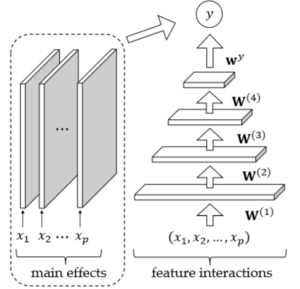
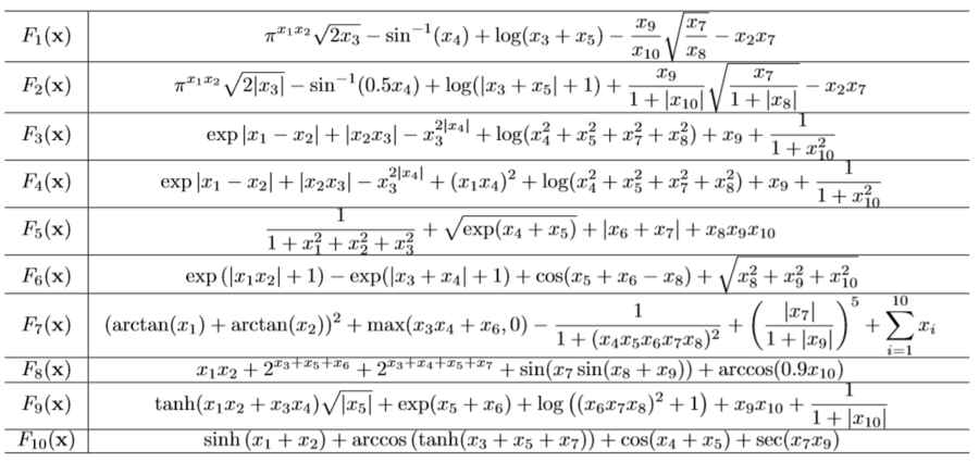
For the experiment, the authors study the interaction detection framework on both simulated and real-world experiments. For simulated experiments, the authors are going to test on 10 synthetic functions as shown in Table I.
The authors use four real-world datasets, of which two are regression datasets, and the other two are binary classification datasets. The datasets are a mixture of common prediction tasks in the cal housing and bike sharing datasets, a scientific discovery task in the higgs boson dataset, and an example of very-high order interaction detection in the letter dataset. Specifically, the cal housing dataset is a regression dataset with 21k data points for predicting California housing prices. The bike sharing dataset contains 17k data points of weather and seasonal information to predict the hourly count of rental bikes in a bike-share system. The Higgs-Boson dataset has 800k data points for classifying whether a particle environment originates from the decay of a Higgs-Boson.
And the authors also reported the results of comparisons between the models. As you can see, neural network based models are performing better on average. Compared to the traditional methods like ANOVA, MLP and MLP-M, proposed method shows 20% increases in performance.
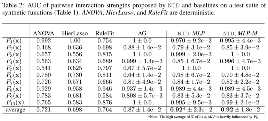
The above result shows that MLP-M almost perfectly capture the most influential pair-wise interactions.
Higher-order interaction detection
The authors use their greedy interaction ranking algorithm to perform higher-order interaction detection without an exponential search of interaction candidates.

Limitations
Even though for the above synthetic experiment MLP methods showed superior performances, the method still has some limitations. For example, for the function like, [math]\displaystyle{ x_1x_2 + x_2x_3 + x_1x_3 }[/math], neural network fails to distinguish between interlinked interactions to single higher order interaction. Moreover, a correlation between features deteriorates the ability of the network to distinguish interactions. However, correlation issues are presented most of interaction detection algorithms.
In the case of detecting pairwise interactions, the interlinked pairwise interactions are often confused by the algorithm for complex interactions. This means that the higher-order interaction algorithm fails to separate interlinked pairwise interactions encoded in the neural network. Another issue is that it sometimes detects abrupt interactions or misses interactions as a result of correlations between features
Because this method relies on the neural network fitting the data well, there are some additional concerns. Notably, if the NN is unable to make an appropriate fit (under/overfitting), the resulting interactions will be flawed. This can occur if the datasets that are too small or too noisy, which often occurs in practical settings.
Conclusion
Here we presented the method of detecting interactions using MLP. Compared to other state-of-the-art methods like Additive Groves (AG), the performances are competitive yet computational powers required is far less. Therefore, it is safe to claim that the method will be extremely useful for practitioners with (comparably) less computational powers. Moreover, the NIP algorithm successfully reduced the computation sizes. After all, the most important aspect of this algorithm is that now users of nueral networks can impose interpretability in the model usage, which will change the level of usability to another level for most of the practitioners outside of those working in machine learning and deep learning areas.
For future work, the authors want to detect feature interactions by using the common units in the intermediate hidden layers of feedforward networks, and also want to use such interaction detection to interpret weights in other deep neural networks. Also, it was pointed out that the neural network weights heavily depend on L-1 regularized neural network training, but a group lasso penalty may work better.
Critique
1. Authors need to do large-scale experiments, instead of just conducting experiments on some synthetic dataset with small feature dimensionality, to make their claim stronger.
2. Although the method proposed in this paper is interesting, the paper would benefit from providing some more explanations to support its idea and fill the possible gaps in its experimental evaluation. In some parts there are repetitive explanations that could be replaced by other essential clarifications.
3. Greedy algorithm is implemented but nothing is mentioned about the speed of this algorithm which is definitely not fast. So, this has the potential to be a weak point of the study.
4. Could have provided more experiments.
Reference
[1] Jacob Bien, Jonathan Taylor, and Robert Tibshirani. A lasso for hierarchical interactions. Annals of statistics, 41(3):1111, 2013.
[2] G David Garson. Interpreting neural-network connection weights. AI Expert, 6(4):46–51, 1991.
[3] Yotam Hechtlinger. Interpretation of prediction models using the input gradient. arXiv preprint arXiv:1611.07634, 2016.
[4] Shiyu Liang and R Srikant. Why deep neural networks for function approximation? 2016.
[5] David Rolnick and Max Tegmark. The power of deeper networks for expressing natural functions. International Conference on Learning Representations, 2018.
[6] Daria Sorokina, Rich Caruana, and Mirek Riedewald. Additive groves of regression trees. Machine Learning: ECML 2007, pp. 323–334, 2007.
[7] Simon Wood. Generalized additive models: an introduction with R. CRC press, 2006
[8] Sebastian Bach, Alexander Binder, Gre ́goire Montavon, Frederick Klauschen, Klaus-Robert Mu ̈ller, and Wojciech Samek. On pixel-wise explanations for non-linear classifier decisions by layer-wise relevance propagation. PloS one, 10(7):e0130140, 2015.
[9] Rich Caruana, Yin Lou, Johannes Gehrke, Paul Koch, Marc Sturm, and Noemie Elhadad. Intel- ligible models for healthcare: Predicting pneumonia risk and hospital 30-day readmission. In Proceedings of the 21th ACM SIGKDD International Conference on Knowledge Discovery and Data Mining, pp. 1721–1730. ACM, 2015.
[10] Zhengping Che, Sanjay Purushotham, Robinder Khemani, and Yan Liu. Interpretable deep models for icu outcome prediction. In AMIA Annual Symposium Proceedings, volume 2016, pp. 371. American Medical Informatics Association, 2016.
[11] Laurent Itti, Christof Koch, and Ernst Niebur. A model of saliency-based visual attention for rapid scene analysis. IEEE Transactions on pattern analysis and machine intelligence, 20(11):1254– 1259, 1998.
[12] Marco Tulio Ribeiro, Sameer Singh, and Carlos Guestrin. Why should i trust you?: Explaining the predictions of any classifier. In Proceedings of the 22nd ACM SIGKDD International Conference on Knowledge Discovery and Data Mining, pp. 1135–1144. ACM, 2016.
[13]Karen Simonyan, Andrea Vedaldi, and Andrew Zisserman. Deep inside convolutional networks: Vi- sualising image classification models and saliency maps. arXiv preprint arXiv:1312.6034, 2013.
[14] Kush R Varshney and Homa Alemzadeh. On the safety of machine learning: Cyber-physical sys- tems, decision sciences, and data products. arXiv preprint arXiv:1610.01256, 2016.
[15] Jason Yosinski, Jeff Clune, Anh Nguyen, Thomas Fuchs, and Hod Lipson. Understanding neural networks through deep visualization. arXiv preprint arXiv:1506.06579, 2015.