Continuous Adaptation via Meta-Learning in Nonstationary and Competitive Environments
Introduction
Typically, the basic goal of machine learning is to train a model to perform a task. In meta-learning, the goal is to train a model to perform the task of training a model to perform a task. Hence, in this case, the term "meta-Learning" has the exact meaning one would expect; the word "meta" has the precise function of introducing a layer of abstraction.
The meta-learning task can be made more concrete by a simple example. Consider the CIFAR-100 classification task that we used for our data competition. We can alter this task from being a 100-class classification problem to a collection of 100 binary classification problems. The goal of meta-learning here is to design and train a single binary classifier for each class that will perform well on a randomly sampled task given a limited amount of training data for that specific task. In other words, we would like to train a model to perform the following procedure:
- A task is sampled. The task is "Is X a dog?".
- A small set of labeled training data is provided to the model. Each label is a boolean representing whether or not the corresponding image is a picture of a dog.
- The model uses the training data to adjust itself to the specific task of checking whether or not an image is a picture of a dog.
This example also highlights the intuition that the skill of sight is distinct and separable from the skill of knowing what a dog looks like.
In this paper, a probabilistic framework for meta-learning is derived, then applied to tasks involving simulated robotic spiders. This framework generalizes the typical machine learning setup using Markov Decision Processes. This paper focuses on a multi-agent non-stationary environment which requires reinforcement learning (RL) agents to do a continuous adaptation in such an environment. Non-stationarity breaks the standard assumptions and requires agents to continuously adapt, both at training and execution time, in order to earn more rewards, hence the approach is to break this into a sequence of stationary tasks and present it as a multi-task learning problem.

Background
Markov Decision Process (MDP)
A MDP is defined by the tuple [math]\displaystyle{ (S,A,P,r,\gamma) }[/math], where S is a set of states, A is a set of actions, P is the transition probability distribution, r is the reward function, and [math]\displaystyle{ \gamma }[/math] is the discount factor. More information (here).
Model Agnostic Meta-Learning
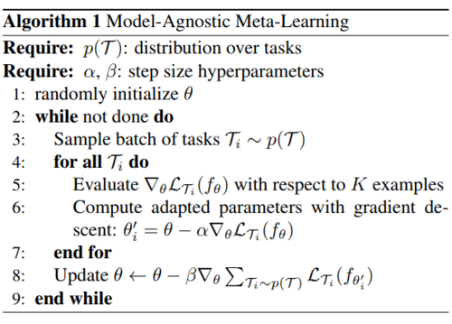
An initial framework for meta-learning is given in "Model-Agnostic Meta-Learning for Fast Adaptation of Deep Networks" (Finn et al, 2017):
"In our approach, the parameters of the model are explicitly trained such that a small number of gradient steps with a small amount of training data from a new task will produce good generalization performance on that task" (Finn et al, 2017).
Where [math]\displaystyle{ \theta }[/math] denotes the meta learning model parameter, and [math]\displaystyle{ \theta_i' }[/math] denotes the model parameter after adapting to Task [math]\displaystyle{ T_i }[/math]
In this training algorithm, the parameter vector [math]\displaystyle{ \theta }[/math] belonging to the model [math]\displaystyle{ f_{\theta} }[/math] is trained such that the meta-objective function [math]\displaystyle{ \mathcal{L} (\theta) = \sum_{\tau_i \sim P(\tau)} \mathcal{L}_{\tau_i} (f_{\theta_i' }) }[/math] is minimized. The sum in the objective function is over a sampled batch of training tasks. [math]\displaystyle{ \mathcal{L}_{\tau_i} (f_{\theta_i'}) }[/math] is the training loss function corresponding to the [math]\displaystyle{ i^{th} }[/math] task in the batch evaluated at the model [math]\displaystyle{ f_{\theta_i'} }[/math]. The parameter vector [math]\displaystyle{ \theta_i' }[/math] is obtained by updating the general parameter [math]\displaystyle{ \theta }[/math] using the loss function [math]\displaystyle{ \mathcal{L}_{\tau_i} }[/math] and set of K training examples specific to the [math]\displaystyle{ i^{th} }[/math] task. Note that in alternate versions of this algorithm, additional testing sets are sampled from [math]\displaystyle{ \tau_i }[/math] and used to update [math]\displaystyle{ \theta }[/math] using testing loss functions instead of training loss functions.
One of the important difference between this algorithm and more typical fine-tuning methods is that [math]\displaystyle{ \theta }[/math] is explicitly trained to be easily adjusted to perform well on different tasks rather than perform well on any specific tasks then fine tuned as the environment changes. (Sutton et al., 2007). In essence, the model is trained so that gradient steps are highly productive at adapting the model parameters to a new enviroment.
Probabilistic Framework for Meta-Learning
This paper puts the meta-learning problem into a Markov Decision Process (MDP) framework common to RL, see Figure 1a. Instead of training examples [math]\displaystyle{ \{(x, y)\} }[/math], we have trajectories [math]\displaystyle{ \tau = (x_0, a_1, x_1, R_1, a_2,x_2,R_2, ... a_H, x_H, R_H) }[/math]. A trajectory is sequence of states/observations [math]\displaystyle{ x_t }[/math], actions [math]\displaystyle{ a_t }[/math] and rewards [math]\displaystyle{ R_t }[/math] that is sampled from a task [math]\displaystyle{ T }[/math] according to a policy [math]\displaystyle{ \pi_{\theta} }[/math]. Included with said task is a method for assigning loss values to trajectories [math]\displaystyle{ L_T(\tau) }[/math] which is typically the negative cumulative reward. A policy is a deterministic function that takes in a state and returns an action. Our goal here is to train a policy [math]\displaystyle{ \pi_{\theta} }[/math] with parameter vector [math]\displaystyle{ \theta }[/math]. This is analougous to training a function [math]\displaystyle{ f_{\theta} }[/math] that assigns labels [math]\displaystyle{ y }[/math] to feature vectors [math]\displaystyle{ x }[/math]. More precisely we have the following definitions:
- [math]\displaystyle{ \tau = (x_0, a_1, x_1, R_1, x_2, ... a_H, x_H, R_H) }[/math] trajectories.
- [math]\displaystyle{ T :=(L_T, P_T(x), P_T(x_t | x_{t-1}, a_{t-1}), H ) }[/math] (A Task)
- [math]\displaystyle{ D(T) }[/math] : A distribution over tasks.
- [math]\displaystyle{ L_T }[/math]: A loss function for the task T that assigns numeric loss values to trajectories.
- [math]\displaystyle{ P_T(x), P_T(x_t | x_{t-1}, a_{t-1}) }[/math]: Probability measures specifying the markovian dynamics of the observations [math]\displaystyle{ x_t }[/math]
- [math]\displaystyle{ H }[/math]: The horizon of the MDP. This is a fixed natural number specifying the lengths of the tasks trajectories.
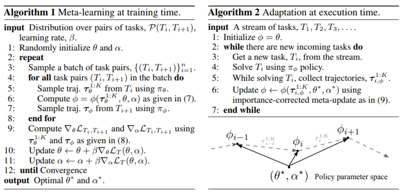
The paper goes further to define a Markov dynamic for sequences of tasks as shown in Figure 1b. Thus the policy that we would like to meta learn [math]\displaystyle{ \pi_{\theta} }[/math], after being exposed to a sample of K trajectories [math]\displaystyle{ \tau_\theta^{1:K} }[/math] from the task [math]\displaystyle{ T_i }[/math], should produce a new policy [math]\displaystyle{ \pi_{\phi} }[/math] that will perform well on the next task [math]\displaystyle{ T_{i+1} }[/math]. Thus we seek to minimize the following expectation:
[math]\displaystyle{ \mathrm{E}_{P(T_0), P(T_{i+1} | T_i)}\bigg(\sum_{i=1}^{l} \mathcal{L}_{T_i, T_{i+1}}(\theta)\bigg) }[/math],
where [math]\displaystyle{ \mathcal{L}_{T_i, T_{i + 1}}(\theta) := \mathrm{E}_{\tau_{i, \theta}^{1:K} } \bigg( \mathrm{E}_{\tau_{i+1, \phi}}\Big( L_{T_{i+1}}(\tau_{i+1, \phi} | \tau_{i, \theta}^{1:K}, \theta) \Big) \bigg) }[/math] and [math]\displaystyle{ l }[/math] is the number of tasks.
The meta-policy [math]\displaystyle{ \pi_{\theta} }[/math] is trained and then adapted at test time using the following procedures. The computational graph is given in Figure 1c.
The mathematics of calculating loss gradients is omitted.
Training Spiders to Run with Dynamic Handicaps (Robotic Locomotion in Non-Stationary Environments)
The authors used the MuJoCo physics simulator to create a simulated environment where robotic spiders with 6 legs are faced with the task of running due east as quickly as possible. The robotic spider observes the location and velocity of its body, and the angles and velocities of its legs. It interacts with the environment by exerting torque on the joints of its legs. Each leg has two joints, the joint closer to the body rotates horizontally while the joint farther from the body rotates vertically. The environment is made non-stationary by gradually paralyzing two legs of the spider across training and testing episodes. This allows the agent to adapt to new environments in each episode. Putting this example into the above probabilistic framework yields:
- [math]\displaystyle{ T_i }[/math]: The task of walking east with the torques of two legs scaled by [math]\displaystyle{ (i-1)/6 }[/math]
- [math]\displaystyle{ \{T_i\}_{i=1}^{7} }[/math]: A sequence of tasks with the same two legs handicapped in each task. Note there are 15 different ways to choose such legs resulting in 15 sequences of tasks. 12 are used for training and 3 for testing.
- A Markov Descision process composed of
- Observations [math]\displaystyle{ x_t }[/math] containing information about the state of the spider.
- Actions [math]\displaystyle{ a_t }[/math] containing information about the torques to apply to the spiders legs.
- Rewards [math]\displaystyle{ R_t }[/math] corresponding to the speed at which the spider is moving east.
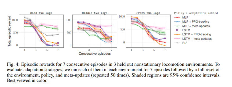
Three differently structured policy neural networks are trained in this set up using both meta-learning and three different previously developed adaption methods.
At testing time, the spiders following meta learned policies initially perform worse than the spiders using non-adaptive policies. However, by the third episode ([math]\displaystyle{ i=3 }[/math]), the meta-learners perform on par. And by the sixth episode, when the selected legs are mostly immobile, the meta-learners significantly out perform. These results can be seen in the graphs below.
Training Spiders to Fight Each Other (Adversarial Meta-Learning)
The authors created an adversarial environment called RoboSumo where pairs of agents with 4 (named Ants), 6 (named Bugs),or 8 legs (named spiders) sumo wrestle. The agents observe the location and velocity of their bodies and the bodies of their opponent, the angles and velocities of their legs, and the forces being exerted on them by their opponent (equivalent of tactile sense). The game is organized into episodes and rounds. Episodes are single wrestling matches with 500 timesteps and win/lose/draw outcomes. Agents win by pushing their opponent out of the ring or making their opponent's body touch the ground. An episode results in a draw when neither of these things happen after 500 timesteps. Rounds are batches of episodes. Rounds have possible outcomes win, lose, and draw that are decided based on majority of episodes won. K rounds will be fought. Both agents may update their policies between rounds. The agent that wins the majority of rounds is deemed the winner of the game.
Setup
Similar to the Robotic locomotion example, this game can be phrased in terms of the RL MDP framework.
- [math]\displaystyle{ T_i }[/math]: The task of fighting a round.
- [math]\displaystyle{ \{T_i\}_{i=1}^{K} }[/math]: A sequence of rounds against the same opponent. Note that the opponent may update their policy between rounds but the anatomy of both wrestlers will be constant across rounds.
- A Markov Descision process composed of
- A horizon [math]\displaystyle{ H = 500*n }[/math] where [math]\displaystyle{ n }[/math] is the number of episodes per round.
- Observations [math]\displaystyle{ x_t }[/math] containing information about the state of the agent and its opponent.
- Actions [math]\displaystyle{ a_t }[/math] containing information about the torques to apply to the agents legs.
- Rewards [math]\displaystyle{ R_t }[/math] rewards given to the agent based on its wrestling performance. [math]\displaystyle{ R_{500*n} = }[/math] +2000 if win episode, -2000 if lose, and -1000 if draw. A discount factor of [math]\displaystyle{ \gamma = 0.995 }[/math] is applied to the rewards.
Note that the above reward set up is quite sparse. Therefore in order to encourage fast training, rewards are introduced at every time step for the following.
- For staying close to the center of the ring.
- For exerting force on the opponents body.
- For moving towards the opponent.
- For the distance of the opponent to the center of the ring.
In addition to the sparse win/lose rewards, the following dense rewards are also introduced in the early training stages to encourage faster learning:
- Quickly push the opponent outside - penalty proportional to the distance of there opponent from the center of the ring.
- Moving towards the opponent - reward proportional to the velocity component towards the opponent.
- Hit the opponent - reward proportional to square root of the total forces exerted on the opponent.
- Control penalty - penalty denoted by [math]\displaystyle{ l_2 }[/math] on actions which lead to jittery/unnatural movements.
This makes sense intuitively as these are reasonable goals for agents to explore when they are learning to wrestle.
Training
The same combinations of policy networks and adaptation methods that were used in the locomotion example are trained and tested here. A family of non-adaptive policies are first trained via self-play and saved at all stages. Self-play simply means the two agents in the training environment use the same policy. All policy versions are saved so that agents of various skill levels can be sampled when training meta-learners. The weights of the different insects were calibrated such that the test win rate between two insects of differing anatomy, who have been trained for the same number of epochs via self-play, is close to 50%.
We can see in the above figure that the weight of the spider had to be increased by almost four times in order for the agents to be evenly matched.
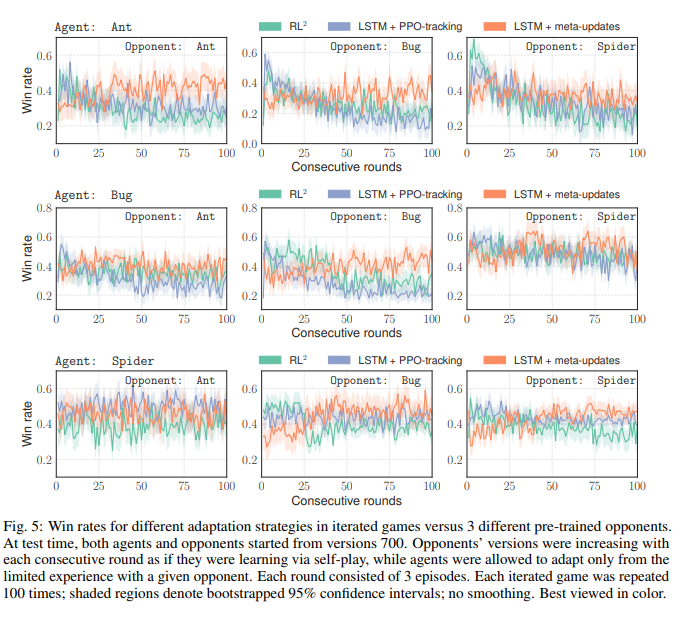
The above figure shows testing results for various adaptation strategies. The agent and opponent both start with the self-trained policies. The opponent uses all of its testing experience to continue training. The agent uses only the last 75 episodes to adapt its policy network. This shows that metal learners need only a limited amount of experience in order to hold their own against a constantly improving opponent.
Evaluating Adaptation Strategies
To compare the proposed strategy against existing strategies, the authors leveraged the Robosumo task to have the different adaptation strategies compete against each other. The scoring metric used is TrueSkill, a metric very similar to ELO. Each strategy starts out with a fixed amount of points. When two different strategies compete the winner gains points and the loser loses points. The number of points gained and lost depend on the different in TrueSkill. A lower ranked opponent defeating a high ranked opponent will gain much more points than a high ranked opponent defeating a lower ranked one. It is assumed that agents skill levels are initially normally distributed with mean 25, and variance 25/3. 1000 matches are generated with each match consisting of 100-round iterated adaptation games. TrueSkill scores are updated after every match. The distribution of TrueSkill after playing 1000 matches are shown below:
In summary recurrent policies are dominant, and the proposed meta-update performs better than or at par with the other strategies.
The authors also demonstrated the same result by starting with 1000 agents, uniformly distributed in terms of adaptation strategies, and randomly matching them against each other for several generations. The loser of each match is removed and replaced with a duplicate of the winner. After several generations, the total population consists mostly of the proposed strategy. This is shown in the figure below.
Future Work
The authors noted that the meta-learning adaptation rule they proposed is similar to backpropagation through time with a unit time lag, so a potential area for future research would be to introduce fully-recurrent meta-updates based on the full interaction history with the environment. Secondly, the algorithm proposed involves computing second-order derivatives at training time (see Figure 1c), which resulted in much slower training processes compared to baseline models during experiments, so they suggested finding a method to utilize information from the loss function without explicit backpropagation to speed up computations. The authors also mention that their approach likely will not work well with sparse rewards. This is because the meta-updates, which use policy gradients, are very dependent on the reward signal. They mention that this is an issue they would like to address in the future. A potential solution they have outlined for this is to introduce auxiliary dense rewards which could enable meta-learning.
Sources
- Chelsea Finn, Pieter Abbeel, Sergey Levine. "Model-Agnostic Meta-Learning for Fast Adaptation of Deep Networks." arXiv preprint arXiv:1703.03400v3 (2017).
- Richard S Sutton, Anna Koop, and David Silver. On the role of tracking in stationary environments. In Proceedings of the 24th international conference on Machine learning, pp. 871–878. ACM, 2007.


