A Bayesian Perspective on Generalization and Stochastic Gradient Descent

Introduction

This paper shows how Bayesian principles can explain many recent observations in the deep learning literature, and provide practical new insights. This work builds on Zhang et al.(2016) who showed that deep convolutional neural networks continue to perform well on the training data even after random relabelling of the input data points, but its ability to generalize and performance on the test data points goes down after the random relabelling. The authors consider two questions: how can we predict if a minimum will generalize to the test set, and why does stochastic gradient descent find minima that generalize well?

The paper shows that the same phenomenon occurs even in small linear models. These observations are explained by the Bayesian evidence, which penalizes sharp minima but is invariant to model parameterization. They also demonstrate that, when one holds the learning rate fixed, there is an optimum batch size which maximizes the test set accuracy.

The authors propose that the noise introduced by small mini-batches drives the parameters towards minima whose evidence is large. Interpreting stochastic gradient descent as a stochastic differential equation, we identify the “noise scale” [math]\displaystyle{ g \approx \epsilon N/B }[/math] where [math]\displaystyle{ ε }[/math] is the learning rate, [math]\displaystyle{ N }[/math] the training set size and [math]\displaystyle{ B }[/math] the batch size. Consequently the optimum batch size is proportional to both the learning rate and the size of the training set, [math]\displaystyle{ B_{opt} \propto \epsilon N }[/math]. The authors verify these predictions empirically.

Motivation and Related Work

Zhang et al. (2016) trained deep convolutional networks on ImageNet and CIFAR10, achieving excellent accuracy on both training and test sets. They then took the same input images, but randomized the labels, and found that while their networks were now unable to generalize to the test set, they still memorized the training labels. They claimed these results contradict learning theory, although this claim is disputed (Kawaguchi et al., 2017; Dziugaite & Roy, 2017). Nonetheless, their results beg the question; if our models can assign arbitrary labels to the training set, why do they work so well in practice?

Meanwhile, Keskar et al. (2016) observed that if we hold the learning rate fixed and increase the batch size, the test accuracy usually falls. This striking result shows improving the estimate of the full-batch gradient can harm performance. Goyal et al. (2017) observed a linear scaling rule between batch size and learning rate in a deep ResNet, while Hoffer et al. (2017) proposed a square root rule on theoretical grounds.

Many authors have suggested “broad minima” whose curvature is small may generalize better than “sharp minima” whose curvature is large (Chaudhari et al., 2016; Hochreiter & Schmidhuber, 1997). Indeed, Dziugaite & Roy (2017) argued the results of Zhang et al. (2016) can be understood using “nonvacuous” PAC-Bayes generalization bounds which penalize sharp minima, while Keskar et al. (2016) showed stochastic gradient descent (SGD) finds wider minima as the batch size is reduced. However, Dinh et al. (2017) challenged this interpretation, by arguing that the curvature of a minimum can be arbitrarily increased by changing the model parameterization.

Contribution

The main contributions of this paper are to show that:

• The results of Zhang et al. (2016) are not unique to deep learning; it is observed the same phenomenon in a small “over-parameterized” linear model. Overparameterization occurs when a model is able to effectively “remember” training data. This occurs when there are enough parameters that the system of equations ends up with an infinite number of possible solutions. One can see why this over-training would lead to poor results in test cases, as this “memorization” learns noise as opposed to the inherent structure of different classes. It is demonstrated that this phenomenon is straightforwardly understood by evaluating the Bayesian evidence in favor of each model, which penalizes sharp minima but is invariant to the model parameterization.
• SGD integrates a stochastic differential equation whose “noise scale” [math]\displaystyle{ g ≈ εN/B }[/math], where [math]\displaystyle{ \epsilon }[/math] is the learning rate, [math]\displaystyle{ N }[/math] training set size, and [math]\displaystyle{ B }[/math] batch size. Noise drives SGD away from sharp minima, and therefore there is an optimal batch size which maximizes the test set accuracy. This optimal batch size is proportional to the learning rate and training set size.

Zhang et al. (2016) showed high training competency of neural networks under informative labels, but drastic overfitting on improper labels. This implies weak generalizability even when a small proportion of labels are improper. The authors show that generalization is strongly correlated with the Bayesian evidence, a weighted combination of the depth of a minimum (the cost function) and its breadth (the Occam factor). Bayesians tend to make distributional assumptions on gradient updates by adding isotropic Gaussian noise. This paper builds upon these Bayesian principles by driving SGD away from sharp minima, and towards broad minima (the more broad, the better generalization due to less influence from small perturbations within input). The stochastic differential equation used as a component of gradient updates effectively serves as injected noise that improves a network's generalizability.

Main Results

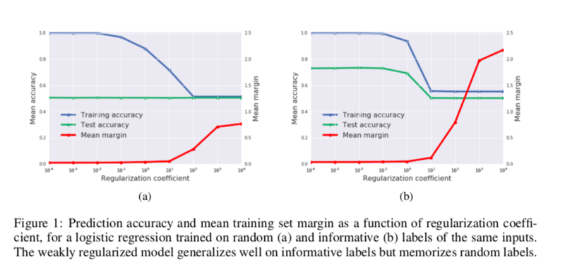
The weakly regularized model memorizes random labels, however, generalizes properly on informative labels. Besides, the predictions are overconfident. The authors also showed that the test accuracy peaks at an optimal batch size, if one holds the other SGD hyper-parameters constant. It is postulated that the optimum represents a tradeoff between depth and breadth in the Bayesian evidence. However, it is the underlying scale of random fluctuations in the SGD dynamics which controls the tradeoff, not the batch size itself. Furthermore, this test accuracy peak shifts as the training set size rises. The authors observed that the best found batch size is proportional to the learning rate. This scaling rule allowed the authors to increase the learning rate by simultaneously increasing the batch size with no loss in test accuracy and no increase in computational cost, thus parallelism across multiple GPU's can be fully leveraged to easily decrease training time. The scaling rule could also be applied to production models by consequentially increasing the batch size as new training data is introduced.

Bayesian Model Comparison

Introduction to Bayesian Statistics

Bayes' theorem is a fundamental theorem in Bayesian statistics, as it is used by Bayesian methods to update probabilities, which are degrees of belief, after obtaining new data. Given two events [math]\displaystyle{ A }[/math] and [math]\displaystyle{ B }[/math], the conditional probability of [math]\displaystyle{ A }[/math] given [math]\displaystyle{ B }[/math] is true, Bayes theorem states that \begin{align*}\displaystyle P(A\mid B)={\frac {P(B\mid A)P(A)}{P(B)}}\end{align*}

Bayesian networks are DAGs whose nodes represent variables in the Bayesian sense: they may be observable quantities, latent variables, unknown parameters or hypotheses. Edges represent conditional dependencies; nodes that are not connected (no path connects one node to another) represent variables that are conditionally independent of each other. Each node is associated with a probability function that takes, as input, a particular set of values for the node's parent variables, and gives (as output) the probability (or probability distribution, if applicable) of the variable represented by the node. For example, if [math]\displaystyle{ m }[/math] parent nodes represent [math]\displaystyle{ m }[/math] Boolean variables then the probability function could be represented by a table of [math]\displaystyle{ 2^{m} }[/math] entries, one entry for each of the [math]\displaystyle{ 2^{m} }[/math] possible parent combinations.

Bayesian Model Comparison in Neural Networks

MacKay (1992) applied Bayesian model comparison to neural networks. An overview is presented below.

We first consider a classification model [math]\displaystyle{ M }[/math] with a single parameter [math]\displaystyle{ \omega }[/math], training inputs [math]\displaystyle{ x }[/math] and training labels [math]\displaystyle{ y }[/math]. We can infer a posterior probability distribution over the parameter by applying Bayes theorem :

\begin{align*}P(\omega\mid y,x;M) = \frac{P(y\mid \omega,x;M)P(\omega;M) }{P(y\mid x;M)}\end{align*}

The likelihood, [math]\displaystyle{ P(y\mid \omega,x;M) = \Pi_i P(y_i\mid \omega,x_i;M) = e^{-H(\omega;M)} }[/math], where [math]\displaystyle{ H(\omega;M) }[/math] denotes the cross-entropy of unique categorical labels. Using a Gaussian prior, [math]\displaystyle{ P(\omega;M) = \sqrt{\lambda/2\pi e^{-\lambda\omega^2/2}} }[/math], and therefore the posterior probability density of the parameter given the training data, [math]\displaystyle{ P(\omega\mid y,x;M) \propto \sqrt{\lambda/2\pi e^{-C(\omega;M)}} }[/math], where [math]\displaystyle{ C(\omega;M) = H(\omega;M) + \lambda\omega^2/2 }[/math] denotes the L2 regularized cross entropy, or “cost function”, and [math]\displaystyle{ \lambda }[/math] is the regularization coefficient.

The value [math]\displaystyle{ \omega_0 }[/math] which minimizes the cost function lies at the maximum of this posterior. To predict an unknown label [math]\displaystyle{ y_t }[/math] of a new input [math]\displaystyle{ x_t }[/math], we should compute the integral,

\begin{align*} P(y_t\mid x_t,y,x;M) &= \int \frac{d\omega P(y_t\mid \omega,x_t;M)}{P(\omega\mid y,x;M)}\\ &= \frac{\int d \omega P(y_t \mid \omega ,x_t;M)e^{-C(\omega;M)}}{\int d \omega e^{-C(\omega;M)}} \end{align*}</math>

However, these integrals are dominated by the region near [math]\displaystyle{ \omega_0 }[/math] . We usually approximate [math]\displaystyle{ P(y_t\mid x_t,x,y;M) \approx P(y_t\mid \omega_0,x_t;M) }[/math]. Having minimized [math]\displaystyle{ C(\omega;M) }[/math] to find [math]\displaystyle{ \omega_0 }[/math], we now wish to compare two different models and select the best one. We use the probability ratio

\begin{align*}\frac{P(M_1\mid y,x)}{P (M_2\mid y, x)} = \frac{P(y\mid x;M_1) P(M_1)}{ P (y\mid x; M_2) P (M_2)} . \end{align*}

The second factor on the right is the prior ratio, which describes which model is most plausible. To avoid unnecessary subjectivity, we usually set this to 1. Meanwhile, the first factor on the right is the evidence ratio, which controls how much the training data changes our prior beliefs

Germain et al. (2016) showed that maximizing the evidence (or “marginal likelihood”) minimizes a PAC-Bayes generalization bound. To compute it, we evaluate \begin{align*}P(y\mid x;M) &= \int d\omega P(y\mid \omega,x;M)P(\omega;M) \\ &=\sqrt{\frac{\lambda}{2\pi}}\int d \omega e^{C(\omega;M)}\end{align*}

Notice that the evidence is computed by integrating out the parameters; and consequently, it is invariant to the model parameterization. Since this integral is dominated by the region near the minimum [math]\displaystyle{ \omega_0 }[/math], we can estimate the evidence by Taylor expanding [math]\displaystyle{ C(\omega; M) \approx C(\omega_0) + C′′(\omega_0)(\omega - \omega_0)^2/2 }[/math]. This gives us

\begin{align*} P(y\mid x;M) &\approx e^{-C(\omega_0)}\sqrt{\frac{\lambda}{2\pi}} \int d \omega e^{-C′′(\omega_0)(\omega - \omega_0)^2/2}\\ &= exp \big\{- C(\omega_0)-\frac{1}{2}\ln(C (\omega_0)/\lambda) \big\}.\end{align*}

The evidence is controlled by the value of the cost function at the minimum, and by the logarithm of the ratio of the curvature about this minimum compared to the regularization constant. In models with many parameters \begin{align*} P(y\mid x;M) &\approx e^{-C(\omega_0)}\sqrt{\frac{\lambda}{2\pi}} \int d \omega e^{-C′′(\omega_0)(\omega - \omega_0)^2/2} \\ &= exp \big\{- C(\omega_0)-\frac{1}{2} \sum_{i=1}^p \ln (\lambda_i/\lambda) \big\}.\end{align*}

Occam’s factor arises from the log ratio [math]\displaystyle{ \ln (\lambda_i/\lambda) }[/math] The Occam factor describes the fraction of the prior parameter space consistent with the data. Occam’s factor penalizes the amount of information the model must learn about the parameters to accurately model the training data. Since the fraction is always less than one, the authors propose to approximate [math]\displaystyle{ P(y\mid x;M) }[/math] away from local minima by only performing the summation over eigenvalues [math]\displaystyle{ \lambda_i \geq \lambda }[/math].

The authors compare evidence against a null model which assumes the labels are entirely random. This model has no parameters, and so the evidence is controlled by the likelihood alone. [math]\displaystyle{ P(y\mid x;NULL) = (1/n)^N = e^{-N \ln(n)} }[/math], where [math]\displaystyle{ n }[/math] denotes the number of model classes and [math]\displaystyle{ N }[/math] the number of training labels. The evidence ratio : \begin{equation*}\frac{P(y\mid x;M) }{P(y\mid x;NULL) } = e ^{-E(\omega_0)} \end{equation*} [math]\displaystyle{ E(\omega_0) = C(\omega_0)-\frac{1}{2} \sum_{i=1}^p \ln (\lambda_i/\lambda) - N\ln (n) }[/math] is the log evidence ratio in favor of the null model. The authors assign confidence to the predictions of a model iff [math]\displaystyle{ E(\omega_0 \lt 0 }[/math].

The evidence supports the intuition that broad minima generalize better than sharp minima, but unlike the curvature, it does not depend on the model parameterization. Dinh et al. (2017) showed one can increase the Hessian eigenvalues by rescaling the parameters, but they must simultaneously rescale the regularization coefficients, otherwise the model changes. Since Occam’s factor arises from the log ratio, [math]\displaystyle{ \ln (\lambda_i/\lambda) }[/math] , these two effects cancel out. Note however that while the evidence itself is invariant to model parameterization, one can find reparameterizations which change the approximate evidence after the Laplace approximation. It is difficult to evaluate the evidence for deep networks, as we cannot compute the Hessian of millions of parameters. Additionally, neural networks exhibit many equivalent minima, since we can permute the hidden units without changing the model. To compute the evidence we must carefully account for this “degeneracy”. The authors argue these issues are not a major limitation, since the intuition they build studying the evidence in simple cases will be sufficient to explain the results of both Zhang et al. (2016) and Keskar et al. (2016).

Bayes Theorem and Generalization

Zhang et al. (2016) showed that deep neural networks generalize well on training inputs with informative labels, but the same model can overfit on the same input images when the labels are randomized; perfectly memorizing the training set. To demonstrate that these observations are not unique to deep network, the authors use logistic regression. They form a small balanced training set comprising 800 images from MNIST, of which half have the true label “0” and half true label “1”. The test set is balanced, comprising 5000 MNIST images of zeros and 5000 MNIST images of ones. There are two tasks. In the first task, the labels of both the training and test sets are randomized. In the second task, the labels are informative, matching the true MNIST labels. The model has 784 weights and 1 bias.

The accuracy of the model predictions on both the training and test sets is shown in figure 1. When trained on the informative labels, the model generalizes well to the test set, so long as it is weakly regularized. However the model also perfectly memorizes the random labels, replicating the observations of Zhang et al. (2016) in deep networks. No significant improvement in model performance is observed as the regularization coefficient increases. For completeness, we also evaluate the mean margin between training examples and the decision boundary. For both random and informative labels, the margin drops significantly as we reduce the regularization coefficient. When weakly regularized, the mean margin is roughly 50% larger for informative labels than for random labels.

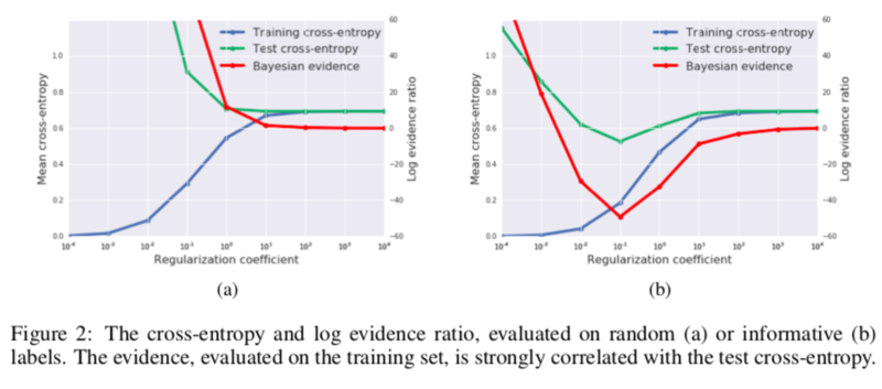
Now consider figure 2, where we plot the mean cross-entropy of the model predictions, evaluated on both training and test sets, as well as the Bayesian log evidence ratio defined in the previous section. Looking first at the random label experiment in figure 2a, while the cross-entropy on the training set vanishes when the model is weakly regularized, the cross-entropy on the test set explodes. Not only does the model make random predictions, but it is extremely confident in those predictions. As the regularization coefficient is increased the test set cross-entropy falls, settling at [math]\displaystyle{ ln(2) }[/math], the cross-entropy of assigning equal probability to both classes. Now consider the Bayesian evidence, which we evaluate on the training set. The log evidence ratio is large and positive when the model is weakly regularized, indicating that the model is exponentially less plausible than assigning equal probabilities to each class. As the regularization parameter is increased, the log evidence ratio falls, but it is always positive, indicating that the model can never be expected to generalize well. Now consider figure 2b (informative labels). Once again, the training cross-entropy falls to zero when the model is weakly regularized, while the test cross-entropy is high. Even though the model makes accurate predictions, those predictions are overconfident. As the regularization coefficient increases, the test cross-entropy falls below ln 2, indicating that the model is successfully generalizing to the test set. Now consider the Bayesian evidence. The log evidence ratio is large and positive when the model is weakly regularized, but as the regularization coefficient increases, the log evidence ratio drops below zero, indicating that the model is exponentially more plausible than assigning equal probabilities to each class. As we further increase the regularization, the log evidence ratio rises to zero while the test cross-entropy rises to [math]\displaystyle{ ln(2) }[/math]. Test cross-entropy and Bayesian evidence are strongly correlated, with minima at the same regularization strength.

Bayesian model comparison has explained our results in a logistic regression. Meanwhile, Krueger et al. (2017) showed the largest Hessian eigenvalue also increased when training on random labels in deep networks, implying the evidence is falling. We conclude that Bayesian model comparison is quantitatively consistent with the results of Zhang et al. (2016) in linear models where we can compute the evidence, and qualitatively consistent with their results in deep networks where we cannot. Dziugaite & Roy (2017) recently demonstrated the results of Zhang et al. (2016) can also be understood by minimising a PAC-Bayes generalization bound which penalizes sharp minima.

Bayes Theorem and Stochastic Gradient Descent

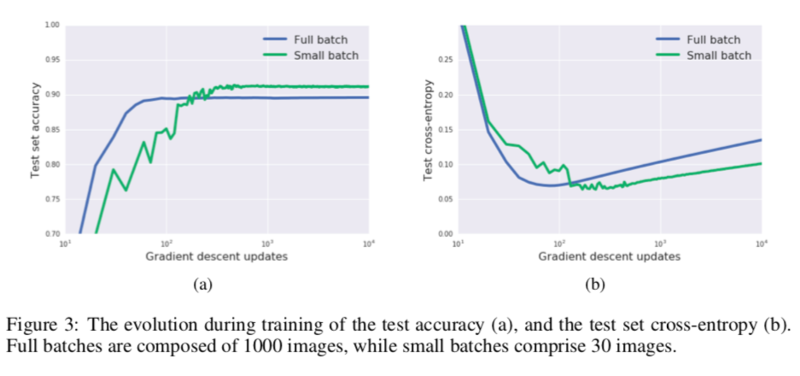
We showed above that generalization is strongly correlated with the Bayesian evidence, a weighted combination of the depth of a minimum (the cost function) and its breadth (the Occam factor). Consequently Bayesians often add isotropic Gaussian noise to the gradient (Welling & Teh, 2011). In appendix A, we show this drives the parameters towards broad minima whose evidence is large. The noise introduced by small batch training is not isotropic, and its covariance matrix is a function of the parameter values, but empirically Keskar et al. (2016) found it has similar effects, driving the SGD away from sharp minima. This paper therefore proposes Bayesian principles also account for the “generalization gap”, whereby the test set accuracy often falls as the SGD batch size is increased (holding all other hyper-parameters constant). Since the gradient drives the SGD towards deep minima, while noise drives the SGD towards broad minima, we expect the test set performance to show a peak at an optimal batch size, which balances these competing contributions to the evidence. We were unable to observe a generalization gap in linear models (since linear models are convex there are no sharp minima to avoid). Instead we consider a shallow neural network with 800 hidden units and RELU hidden activations, trained on MNIST without regularization. We use SGD with a momentum parameter of 0.9. Unless otherwise stated, we use a constant learning rate of 1.0 which does not depend on the batch size or decay during training. Furthermore, we train on just 1000 images, selected at random from the MNIST training set. This enables us to compare small batch to full batch training. We emphasize that we are not trying to achieve optimal performance, but to study a simple model which shows a generalization gap between small and large batch training. In figure 3, we exhibit the evolution of the test accuracy and test cross-entropy during training. Our small batches are composed of 30 images, randomly sampled from the training set. Looking first at figure 3a, small batch training takes longer to converge, but after a thousand gradient updates a clear generalization gap in model accuracy emerges between small and large training batches. Now consider figure 3b. While the test cross-entropy for small batch training is lower at the end of training; the cross-entropy of both small and large training batches is increasing, indicative of over-fitting. Both models exhibit a minimum test cross-entropy, although after different numbers of gradient updates. Intriguingly, we show in appendix B that the generalization gap between small and large batch training shrinks significantly when we introduce L2 regularization.

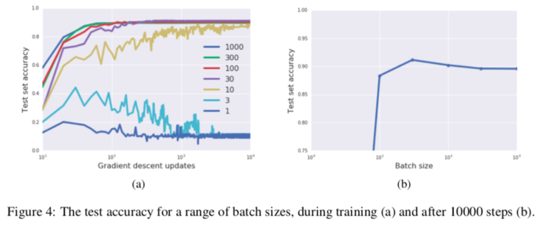
From now on we focus on the test set accuracy (since this converges as the number of gradient updates increases). In figure 4a, we exhibit training curves for a range of batch sizes between 1 and 1000. We find that the model cannot train when the batch size [math]\displaystyle{ B \leq 10 }[/math]. In figure 4b we plot the mean test set accuracy after 10,000 training steps. A clear peak emerges, indicating that there is indeed an optimum batch size which maximizes the test accuracy, consistent with Bayesian intuition. The results of Keskar et al. (2016) focused on the decay in test accuracy above this optimum batch size.

Stochastic Differential Equations and Scaling Rules

The results showed above indicate that the test accuracy peaks at an optimal batch size, if one holds the other SGD hyper-parameters constant. It is argued that this peak arises from the tradeoff between depth and breadth in the Bayesian evidence. However it is not the batch size itself which controls this tradeoff, but the underlying scale of random fluctuations in the SGD dynamics. The following content identifies this SGD “noise scale”, and uses it to derive three scaling rules which predict how the optimal batch size depends on the learning rate, training set size and momentum coefficient. First, interpret gradient update, as the discrete update of a stochastic differential equation \begin{equation*}\frac{d\omega}{dt} = \frac{dC}{d\omega} + \eta(t)\end{equation*} [math]\displaystyle{ \eta }[/math] represents noise [math]\displaystyle{ \langle \eta(t) \rangle = 0 }[/math] and [math]\displaystyle{ \langle \eta (t)\eta (t')\rangle = gF (\omega)\delta (t-t') }[/math]. [math]\displaystyle{ t }[/math] is a continous variable, and [math]\displaystyle{ F(\omega) }[/math] matrix describing the gradient covariances. The SGD noise scale is taken to be [math]\displaystyle{ g \approx \epsilon N/B }[/math] where [math]\displaystyle{ \epsilon }[/math] is the learning rate, [math]\displaystyle{ N }[/math] training set size and [math]\displaystyle{ B }[/math] the batch size.

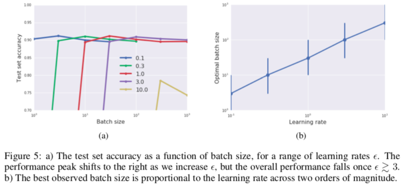
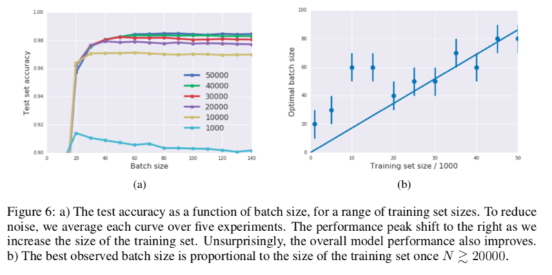
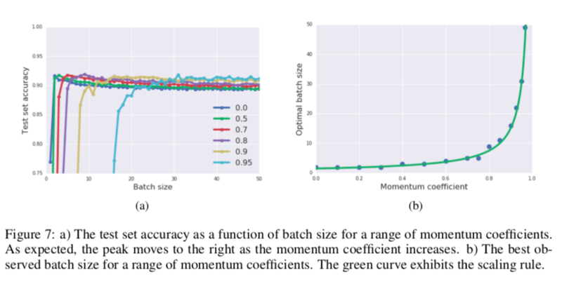
The noise scale falls when the batch B size increases, consistent with our earlier observation of an optimal batch size Bopt while holding the other hyper-parameters fixed. Notice that one would equivalently observe an optimal learning rate if one held the batch size constant. A similar analysis of the SGD was recently performed by Mandt et al. (2017), although their treatment only holds near local minima where the covariances [math]\displaystyle{ F (ω) }[/math] are stationary. Our analysis holds throughout training, which is necessary since Keskar et al. (2016) found that the beneficial influence of noise was most pronounced at the start of training. When we vary the learning rate or the training set size, we should keep the noise scale fixed, which implies that [math]\displaystyle{ Bopt ∝ εN }[/math]. In figure 5a, we plot the test accuracy as a function of batch size after [math]\displaystyle{ (10000/ε) }[/math] training steps, for a range of learning rates. Exactly as predicted, the peak moves to the right as [math]\displaystyle{ ε }[/math] increases. Additionally, the peak test accuracy achieved at a given learning rate does not begin to fall until [math]\displaystyle{ ε ∼ 3 }[/math], indicating that there is no significant discretization error in integrating the stochastic differential equation below this point. Above this point, the discretization error begins to dominate and the peak test accuracy falls rapidly. In figure 5b, we plot the best observed batch size as a function of learning rate, observing a clear linear trend, [math]\displaystyle{ Bopt ∝ ε }[/math]. The error bars indicate the distance from the best observed batch size to the next batch size sampled in our experiments.

This scaling rule allows us to increase the learning rate with no loss in test accuracy and no increase in computational cost, simply by simultaneously increasing the batch size. We can then exploit increased parallelism across multiple GPUs, reducing model training times (Goyal et al., 2017). A similar scaling rule was independently proposed by Jastrzebski et al. (2017) and Chaudhari & Soatto (2017), although neither work identifies the existence of an optimal noise scale. A number of authors have proposed adjusting the batch size adaptively during training (Friedlander & Schmidt, 2012; Byrd et al., 2012; De et al., 2017), while Balles et al. (2016) proposed linearly coupling the learning rate and batch size within this framework. In Smith et al. (2017), we show empirically that decaying the learning rate during training and increasing the batch size during training are equivalent. In figure 6a we exhibit the test set accuracy as a function of batch size, for a range of training set sizes after 10000 steps ([math]\displaystyle{ ε = 1 }[/math] everywhere). Once again, the peak shifts right as the training set size rises, although the generalization gap becomes less pronounced as the training set size increases. In figure 6b, we plot the best observed batch size as a function of training set size; observing another linear trend, [math]\displaystyle{ Bopt ∝ N }[/math]. This scaling rule could be applied to production models, progressively growing the batch size as new training data is collected. We expect production datasets to grow considerably over time, and consequently large batch training is likely to become increasingly common. [math]\displaystyle{ B(1−m) }[/math] scale of conventional SGD as [math]\displaystyle{ m → 0 }[/math]. When [math]\displaystyle{ m \gt 0 }[/math], we obtain an additional scaling rule [math]\displaystyle{ Bopt ∝ 1/(1 − m) }[/math]. This scaling rule predicts that the optimal batch size will increase when the momentum coefficient is increased. In figure 7a we plot the test set performance as a function of batch size after 10000 gradient updates ([math]\displaystyle{ ε = 1 }[/math] everywhere), for a range of momentum coefficients. In figure 7b, we plot the best observed batch size as a function of the momentum coefficient, and fit our results to the scaling rule above; obtaining remarkably good agreement.

Critiques

1. Bayesian statistics is not provably, at present, a theory that can be used to explain why a learning algorithm works. The Bayesian theory is too optimistic: we introduce a prior and model and then trust both implicitly. Relative to any particular prior and model (likelihood), the Bayesian posterior is the optimal summary of the data, but if either part is misspecified, then the Bayesian posterior carries no optimality guarantee. The prior is chosen for convenience here.
2. No discussions with respect to the analysis of information bottleneck which also discuss the generalization ability of the model.
3. No discussion on real online learning with streaming data where the total number of data points are unknown?
4. The paper presents how mini-batch noises with SGD can improve the performance of neural networks. However, the usefulness of the approach can be described and analyzed in greater details, if the author could provide the performance for various well-known real-life data.

Conclusion

The paper showed that mini-batch noise helps SGD to go away from sharp minima, and provided an evidence that there is an optimal optimum batch size for a maximum the test accuracy. Based on interpreting SGD as integrating stochastic differential equation, this batch size is proportional to the learning rate and the training set size. Moreover, the authors shown that [math]\displaystyle{ Bopt \propto 1/(1 − m) }[/math], where [math]\displaystyle{ m }[/math] is the momentum coefficient. More analysis was done on the relation between the learning rate, effective learning rate, and batch size is presented in ICLR 2018, where the authors proved by experiments that all the benefits of decaying the learning rate are achieved by increasing the batch size in addition to reducing the number of parameter updates dramatically, and also were able use literature parameters without the need of any hyper parameter tuning (Samuel L. Smith, Pieter-Jan Kindermans, Chris Ying, Quoc V. Le).

References

1. Alessandro Achille and Stefano Soatto. On the emergence of invariance and disentangling in deep representations. arXiv preprint arXiv:1706.01350, 2017.
2. Lukas Balles, Javier Romero, and Philipp Hennig. Coupling adaptive batch sizes with learning rates. arXiv preprint arXiv:1612.05086, 2016.
3. Richard H Byrd, Gillian M Chin, Jorge Nocedal, and Yuchen Wu. Sample size selection in optimization methods for machine learning. Mathematical programming, 134(1):127–155, 2012.
4. Pratik Chaudhari and Stefano Soatto. Stochastic gradient descent performs variational inference converges to limit cycles for deep networks. arXiv preprint arXiv:1710.11029, 2017.
5. Pratik Chaudhari, Anna Choromanska, Stefano Soatto, and Yann LeCun. Entropy-SGD: Biasing gradient descent into wide valleys. arXiv preprint arXiv:1611.01838, 2016.
6. Soham De, Abhay Yadav, David Jacobs, and Tom Goldstein. Automated inference with adaptive batches. In Artificial Intelligence and Statistics, pp. 1504–1513, 2017.
7. Laurent Dinh, Razvan Pascanu, Samy Bengio, and Yoshua Bengio. Sharp minima can generalize for deep nets. arXiv preprint arXiv:1703.04933, 2017.
8. Gintare Karolina Dziugaite and Daniel M Roy. Computing nonvacuous generalization bounds for deep (stochastic) neural networks with many more parameters than training data. arXiv preprint arXiv:1703.11008, 2017.
9. Michael P Friedlander and Mark Schmidt. Hybrid deterministic-stochastic methods for data fitting. SIAM Journal on Scientific Computing, 34(3):A1380–A1405, 2012.
10. Crispin W Gardiner. Handbook of Stochastic Methods, volume 4. Springer Berlin, 1985.
11. Pascal Germain, Francis Bach, Alexandre Lacoste, and Simon Lacoste-Julien. PAC-bayesian theory meets bayesian inference. In Advances in Neural Information Processing Systems, pp. 1884– 1892, 2016.
12. Priya Goyal, Piotr Dolla ́r, Ross Girshick, Pieter Noordhuis, Lukasz Wesolowski, Aapo Kyrola, An- drew Tulloch, Yangqing Jia, and Kaiming He. Accurate, large minibatch SGD: Training imagenet in 1 hour. arXiv preprint arXiv:1706.02677, 2017.
13. Stephen F Gull. Bayesian inductive inference and maximum entropy. In Maximum-entropy and Bayesian methods in science and engineering, pp. 53–74. Springer, 1988.
14. Geoffrey E Hinton and Drew Van Camp. Keeping the neural networks simple by minimizing the description length of the weights. In Proceedings of the sixth annual conference on Computational learning theory, pp. 5–13. ACM,1993.
15. Sepp Hochreiter and Ju ̈rgen Schmidhuber. Flat minima. Neural Computation, 9(1):1–42, 1997. Elad Hoffer, Itay Hubara, and Daniel Soudry. Train longer, generalize better: closing the generalization gap in large batch training of neural networks. arXiv preprint arXiv:1705.08741, 2017.
16. Stanisław Jastrzebski, Zachary Kenton, Devansh Arpit, Nicolas Ballas, Asja Fischer, Yoshua Bengio, and Amos Storkey. Three factors influencing minima in SGD. arXiv preprint arXiv:1711.04623, 2017.
17. Robert E Kass and Adrian E Raftery. Bayes factors. Journal of the american statistical association, 90(430):773–795, 1995.
18. Kenji Kawaguchi, Leslie Pack Kaelbling, and Yoshua Bengio. Generalization in deep learning. arXiv preprint arXiv:1710.05468, 2017.
19. Nitish Shirish Keskar, Dheevatsa Mudigere, Jorge Nocedal, Mikhail Smelyanskiy, and Ping Tak Pe- ter Tang. On large-batch training for deep learning: Generalization gap and sharp minima. arXiv preprint arXiv:1609.04836, 2016.
20. David Krueger, Nicolas Ballas, Stanislaw Jastrzebski, Devansh Arpit, Maxinder S Kanwal, Tegan Maharaj, Emmanuel Bengio, Asja Fischer, and Aaron Courville. Deep nets don’t learn via mem- orization. ICLR Workshop, 2017.
21. Qianxiao Li, Cheng Tai, and E Weinan. Stochastic modified equations and adaptive stochastic gradient algorithms. In International Conference on Machine Learning, pp. 2101–2110, 2017.
22. David JC MacKay. A practical bayesian framework for backpropagation networks. Neural compu- tation, 4(3):448–472, 1992.
23. Stephan Mandt, Matthew D Hoffman, and David M Blei. Stochastic gradient descent as approximate bayesian inference. arXiv preprint arXiv:1704.04289, 2017.
24. Ravid Shwartz-Ziv and Naftali Tishby. Opening the black box of deep neural networks via informa- tion. arXiv preprint arXiv:1703.00810, 2017.
25. Samuel L. Smith, Pieter-Jan Kindermans, and Quoc V. Le. Don’t decay the learning rate, increase the batch size. arXiv preprint arXiv:1711.00489, 2017.
26. Max Welling and Yee W Teh. Bayesian learning via stochastic gradient langevin dynamics. In Proceedings of the 28th International Conference on Machine Learning (ICML-11), pp. 681–688, 2011.
27. Chiyuan Zhang, Samy Bengio, Moritz Hardt, Benjamin Recht, and Oriol Vinyals. Understanding deep learning requires rethinking generalization. arXiv preprint arXiv:1611.03530, 2016.