neural Turing Machines
Neural Turing Machines
Even though recurrent neural networks (RNNs) are Turing complete in theory, the control of logical flow and usage of external memory have been largely ignored in the machine learning literature. This might be due to the fact that the RNNs have to be wired properly to achieve the Turing completeness and this is not necessarily easy to achieve in practice. By adding an addressable memory Graves et al. try to overcome this limitation and name their approach Neural Turing Machine (NTM) as analogy to Turing machines that are finite-state machines extended with an infinite memory. Furthermore, every component of an NTM is differentiable and can, thus, be learned.
Architecture
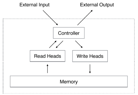
A Neural Turing Machine consists of a memory and a controller neural network. The controller receives input and produces output with help of the memory that is addressed with a content- and location based addressing mechanism. Figure 1 presents a high-level diagram of the NTM architecture.

Memory
The memory at time [math]\displaystyle{ t }[/math] is given by an [math]\displaystyle{ N \times M }[/math] matrix [math]\displaystyle{ M_t }[/math], where [math]\displaystyle{ N }[/math] is the number of memory locations and [math]\displaystyle{ M }[/math] the vector size at each memory location. To address memory locations for reading or writing an [math]\displaystyle{ N }[/math]-element vector [math]\displaystyle{ w_t }[/math] is used. The elements in this vector need to satisfy [math]\displaystyle{ 0 \leq w_t(i) \leq 1 }[/math] and have to sum to 1. Thus, it gives weighting of memory locations and the access to a location might be blurry.
Reading
Given an address [math]\displaystyle{ w_t }[/math] the read vector is just the weighted sum of memory locations:
[math]\displaystyle{ r_t \leftarrow \sum_i w_t(i) M_t(i) }[/math]
Writing
The write process is split up into an erase and an add operation (inspired by the input and forget gates in LSTM). This allows the NTM to both overwrite or add to a memory location in a single time step. Otherwise it would be necessary to do a read for one of the operations first before the updated result can be written.
The erase update is given by
[math]\displaystyle{ \tilde{M}_t(i) \leftarrow M_{t-1}(i) [1 - w_t(i) e_t] }[/math]
with an [math]\displaystyle{ M }[/math]-element erase vector [math]\displaystyle{ e_t }[/math] with elements in the range [math]\displaystyle{ (0, 1) }[/math] selecting which vector elements to reset at the memory locations selected by [math]\displaystyle{ w_t }[/math].
Afterwords an add vector [math]\displaystyle{ a_t }[/math] is added according to
[math]\displaystyle{ M_t(i) \leftarrow \tilde{M}_t(i) + w_t(i) a_t. }[/math]
Addressing Mechanisms
Two methods, content-based addressing and location-based addressing, are employed to generate the read/write weightings [math]\displaystyle{ w_t }[/math]. Depending on the task either mechanism can be more appropriate.
Content-based addressing
For content-addressing, each head (whether employed for reading or writing) first produces a length [math]\displaystyle{ M }[/math] key vector [math]\displaystyle{ k_t }[/math] that is compared to each vector [math]\displaystyle{ M_t (i) }[/math] by a similarity measure [math]\displaystyle{ K[.,.] }[/math]. The content-based system produces a normalised weighting [math]\displaystyle{ w_c^t }[/math] based on the similarity and a positive key strength, [math]\displaystyle{ \beta_t }[/math], which can amplify or attenuate the precision of the focus:
[math]\displaystyle{
w_c^t \leftarrow \frac{exp(\beta_t K[K_t,M_t(i)])}{\sum_{j} exp(\beta_t K[K_t,M_t(j)])}
}[/math]
In this current implementation, the similarity measure is cosine similarity:
[math]\displaystyle{ K[u,v] = \frac{u.v}{||u||.||v||} }[/math]
Location-based addressing
The location-based addressing mechanism is designed to facilitate both simple iterations across the locations of the memory and random-access jumps. It does so by implementing a rotational shift of a weighting. Prior to rotation, each head emits a scalar interpolation gate [math]\displaystyle{ g_t }[/math] in the range (0, 1). The value of [math]\displaystyle{ g }[/math] is used to blend between the weighting [math]\displaystyle{ w_{t-1} }[/math] produced by the head at the previous time-step and the weighting [math]\displaystyle{ w_t^c }[/math] produced by the content system at the current time-step, yielding the gated weighting [math]\displaystyle{ w_t^g }[/math] :
[math]\displaystyle{ w_t^g \leftarrow g_t w_t^c + (1-g_t) w_{t-1} }[/math]
After interpolation, each head emits a shift weighting [math]\displaystyle{ s_t }[/math] that defines a normalised distribution over the allowed integer shifts. Each element in this vector gives the degree by which different integer shifts are performed. For example, if shifts of -1, 0, 1 are allowed a (0, 0.3, 0.7) shift vector would denote a shift of 1 with strength 0.7 and a shift of 0 (no-shift) with strength 0.3. The actual shift is performed with a circular convolution
[math]\displaystyle{ \tilde{w}_t(i) \leftarrow \sum_{j=0}^{N-1} w_t^g(j) s_t(i - j) }[/math]
where all index arithmetic is modulo N. This circular convolution can lead to blurring of the weights and [math]\displaystyle{ _t }[/math] will be sharpened with
[math]\displaystyle{ w_t(i) \leftarrow \frac{\tilde{w}_t(i)^{\gamma_t}}{\sum_j \tilde{w}_t(j)^{\gamma_t}} }[/math]
where [math]\displaystyle{ _t 1 }[/math] is an additional scalar outputted by the write head.
Controller
The controller receives the external input and read head output and produces the addressing vectors and related values (for example shift weighting) for the read and write heads. It also produces an external output.
Different types of controllers can be used. The paper discusses feed-forward and LSTM controllers. Feed-forward controllers are simpler, but are more limited than LSTM controllers since the type of operations they can perform are limited by the number of concurrent read and write heads. The LSTM controller, given it's internal register-like memory, does not suffer from this limitation.
Results
The authors tested the NTM with a feed-forward and an LSTM controller against a pure LSTM on multiple tasks:
- Copy Task: An input sequence has to reproduced.
- Repeat Copy Task: An input sequence has to reproduced multiple times.
- Associative Recall: After providing an input sequence the network is queried with one item of the sequence and has to produce the next.
- Dynamic N-Grams: Predict the probability of the next bit being 0 or 1 given the last six bits.
- Priority Sort: Sort an input sequence according to given priorities.
In all tasks the NTM learns more quickly and gives better generalization than the pure LSTM.