conditional neural process
Introduction
To train a model effectively, deep neural networks typically require large datasets. To mitigate this data efficiency problem, learning in two phases is one approach: the first phase learns the statistics of a generic domain without committing to a specific learning task; the second phase learns a function for a specific task, but does so using only a small number of data points by exploiting the domain-wide statistics already learned. Taking a probabilistic stance and specifying a distribution over functions (stochastic processes) is another approach -- Gaussian Processes being a commonly used example of this. Such Bayesian methods can be computationally expensive, however.
The authors of the paper propose a family of models that represent solutions to the supervised problem, and an end-to-end training approach to learning them that combines neural networks with features reminiscent of Gaussian Processes. They call this family of models Conditional Neural Processes (CNPs). CNPs can be trained on very few data points to make accurate predictions, while they also have the capacity to scale to complex functions and large datasets.
Model
Consider a data set [math]\displaystyle{ \{x_i, y_i\} }[/math] with evaluations [math]\displaystyle{ y_i = f(x_i) }[/math] for some unknown function [math]\displaystyle{ f }[/math]. Assume [math]\displaystyle{ g }[/math] is an approximating function of f. The aim is yo minimize the loss between [math]\displaystyle{ f }[/math] and [math]\displaystyle{ g }[/math] on the entire space [math]\displaystyle{ X }[/math]. In practice, the routine is evaluated on a finite set of observations.
Let training set be [math]\displaystyle{ O = \{x_i, y_i\}_{i = 0} ^{n-1} }[/math], and test set be [math]\displaystyle{ T = \{x_i, y_i\}_{i = n} ^ {n + m - 1} }[/math].
P be a probability distribution over functions [math]\displaystyle{ F : X \to Y }[/math], formally known as a stochastic process. Thus, P defines a joint distribution over the random variables [math]\displaystyle{ {f(x_i)}_{i = 0} ^{n + m - 1} }[/math]. Therefore, for [math]\displaystyle{ P(f(x)|O, T) }[/math], our task is to predict the output values [math]\displaystyle{ f(x_i) }[/math] for [math]\displaystyle{ x_i \in T }[/math], given [math]\displaystyle{ O }[/math],
Conditional Neural Process
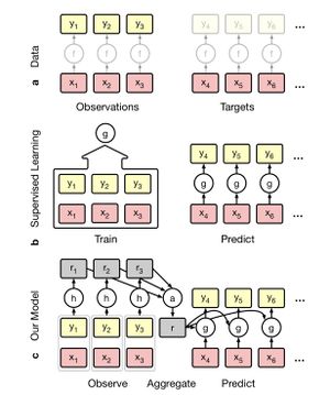
Conditional Neural Process models directly parametrize conditional stochastic processes without imposing consistency with respect to some prior process. CNP parametrize distributions over [math]\displaystyle{ f(T) }[/math] given a distributed representation of [math]\displaystyle{ O }[/math] of fixed dimensionality. Thus, the mathematical guarantees associated with stochastic processes is traded off for functional flexibility and scalability.
CNP is a conditional stochastic process [math]\displaystyle{ Q_\theta }[/math] defines distributions over [math]\displaystyle{ f(x_i) }[/math] for [math]\displaystyle{ x_i \in T }[/math]. For stochastic processs, we assume [math]\displaystyle{ Q_{\theta} }[/math] is invariant to permutations, and in this work, we generally enforce permutation invariance with respect to [math]\displaystyle{ T }[/math] be assuming a factored structure. That is, [math]\displaystyle{ Q_\theta(f(T) | O, T) = \prod _{x \in T} Q_\theta(f(x) | O, x) }[/math]
In detail, we use the following archiecture
[math]\displaystyle{ r_i = h_\theta(x_i, y_i) }[/math] for any [math]\displaystyle{ (x_i, y_i) \in O }[/math], where [math]\displaystyle{ h_\theta : X \times Y \to \mathbb{R} ^ d }[/math]
[math]\displaystyle{ r = r_i * r_2 * ... * r_n }[/math], where [math]\displaystyle{ * }[/math] is a commutative operation that takes elements in [math]\displaystyle{ \mathbb{R}^d }[/math] and maps them into a single element of [math]\displaystyle{ \mathbb{R} ^ d }[/math]
[math]\displaystyle{ \Phi_i = g_\theta }[/math] for any [math]\displaystyle{ x_i \in T }[/math], where [math]\displaystyle{ g_\theta : X \times \mathbb{R} ^ d \to \mathbb{R} ^ e }[/math] and [math]\displaystyle{ \Phi_i }[/math] are parameters for [math]\displaystyle{ Q_\theta }[/math]
Note that this architecture ensures permutation invariance and [math]\displaystyle{ O(n + m) }[/math] scaling for conditional prediction. Also, [math]\displaystyle{ r = r_i * r_2 * ... * r_n }[/math] can be computed in [math]\displaystyle{ O(n) }[/math], this architecture supports streaming observation with minimal overhead.
We train [math]\displaystyle{ Q_\theta }[/math] by asking it to predict [math]\displaystyle{ O }[/math] conditioned on a randomly
chosen subset of [math]\displaystyle{ O }[/math]. This gives the model a signal of the uncertainty over the space X inherent in the distribution
P given a set of observations. Thus, the targets it scores [math]\displaystyle{ Q_\theta }[/math] on include both the observed
and unobserved values. In practice, we take Monte Carlo
estimates of the gradient of this loss by sampling [math]\displaystyle{ f }[/math] and [math]\displaystyle{ N }[/math].
This approach shifts the burden of imposing prior knowledge
from an analytic prior to empirical data. This has the advantage of liberating a practitioner from having to specify an analytic form for the prior, which is ultimately intended to summarize their empirical experience. Still, we emphasize that the [math]\displaystyle{ Q_\theta }[/math] are not necessarily a consistent set of conditionals for all observation sets, and the training routine does not guarantee that.
In summary,
1. A CNP is a conditional distribution over functions trained to model the empirical conditional distributions of functions [math]\displaystyle{ f \sim P }[/math].
2. A CNP is permutation invariant in [math]\displaystyle{ O }[/math] and [math]\displaystyle{ T }[/math].
3. A CNP is scalable, achieving a running time complexity of [math]\displaystyle{ O(n + m) }[/math] for making [math]\displaystyle{ m }[/math] predictions with [math]\displaystyle{ n }[/math] observations.
Experimental Result I: Function Regression
Classical 1D regression task that used as a common baseline for GP is our first example. They generated two different datasets that consisted of functions generated from a GP with an exponential kernel. In the first dataset they used a kernel with fixed parameters, and in the second dataset the function switched at some random point. on the real line between two functions each sampled with different kernel parameters. At every training step they sampled a curve from the GP, select a subset of n points as observations, and a subset of t points as target points. Using the model, the observed points are encoded using a three layer MLP encoder h with a 128 dimensional output representation. The representations are aggregated into a single representation [math]\displaystyle{ r = \frac{1}{n} \sum r_i }[/math] , which is concatenated to [math]\displaystyle{ x_t }[/math] and passed to a decoder g consisting of a five layer MLP.
Two examples of the regression results obtained for each of the datasets are shown in the following figure.
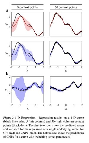
They compared the model to the predictions generated by a GP with the correct hyperparameters, which constitutes an upper bound on our performance. Although the prediction generated by the GP is smoother than the CNP's prediction both for the mean and variance, the model is able to learn to regress from a few context points for both the fixed kernels and switching kernels. As the number of context points grows, the accuracy of the model improves and the approximated uncertainty of the model decreases. Crucially, we see the model learns to estimate its own uncertainty given the observations very accurately. Nonetheless it provides a good approximation that increases in accuracy as the number of context points increases. Furthermore the model achieves similarly good performance on the switching kernel task. This type of regression task is not trivial for GPs whereas in our case we only have to change the dataset used for training
Experimental Result II: Image Completion for Digits
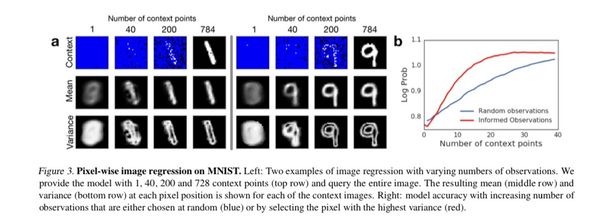
They also tested CNP on the MNIST dataset and use the test set to evaluate its performance. As shown in the above figure the model learns to make good predictions of the underlying digit even for a small number of context points. Crucially, when conditioned only on one non-informative context point the model’s prediction corresponds to the average over all MNIST digits. As the number of context points increases the predictions become more similar to the underlying ground truth. This demonstrates the model’s capacity to extract dataset specific prior knowledge. It is worth mentioning that even with a complete set of observations the model does not achieve pixel-perfect reconstruction, as we have a bottleneck at the representation level. Since this implementation of CNP returns factored outputs, the best prediction it can produce given limited context information is to average over all possible predictions that agree with the context. An alternative to this is to add latent variables in the model such that they can be sampled conditioned on the context to produce predictions with high probability in the data distribution.
An important aspect of the model is its ability to estimate
the uncertainty of the prediction. As shown in the bottom
row of the above figure, as they added more observations, the variance
shifts from being almost uniformly spread over the digit
positions to being localized around areas that are specific
to the underlying digit, specifically its edges. Being able to
model the uncertainty given some context can be helpful for
many tasks. One example is active exploration, where the
model has a choice over where to observe.
They tested this by
comparing the predictions of CNP when the observations
are chosen according to uncertainty, versus random pixels. This method is a very simple way of doing active
exploration, but it already produces better prediction results
than selecting the conditioning points at random.
Experimental Result III: Image Completion for Faces
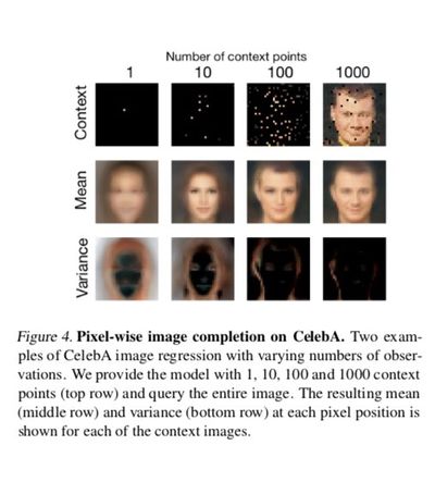
They also applied CNP to CelebA, a dataset of images of
celebrity faces, and reported performance obtained on the
test set.
As shown in the above figure our model is able to capture the complex shapes and colours of this dataset with predictions conditioned on less than 10% of the pixels being already close to ground truth. As before, given few context points the model averages over all possible faces, but as the number of context pairs increases the predictions capture image-specific details like face orientation and facial expression. Furthermore, as the number of context points increases the variance is shifted towards the edges in the image.
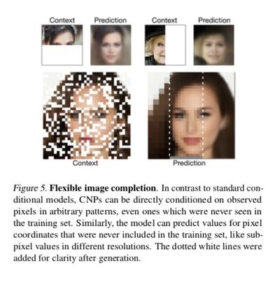
An important aspect of CNPs demonstrated in the above figure is its flexibility not only in the number of observations and targets it receives but also with regards to their input values. It is interesting to compare this property to GPs on one hand, and to trained generative models (van den Oord et al., 2016; Gregor et al., 2015) on the other hand. The first type of flexibility can be seen when conditioning on subsets that the model has not encountered during training. Consider conditioning the model on one half of the image, fox example. This forces the model to not only predict pixel values according to some stationary smoothness property of the images, but also according to global spatial properties, e.g. symmetry and the relative location of different parts of faces. As seen in the first row of the figure, CNPs are able to capture those properties. A GP with a stationary kernel cannot capture this, and in the absence of observations would revert to its mean (the mean itself can be non-stationary but usually this would not be enough to capture the interesting properties).
In addition, the model is flexible with regards to the target input values. This means, e.g., we can query the model at resolutions it has not seen during training. We take a model that has only been trained using pixel coordinates of a specific resolution, and predict at test time subpixel values for targets between the original coordinates. As shown in Figure 5, with one forward pass we can query the model at different resolutions. While GPs also exhibit this type of flexibility, it is not the case for trained generative models, which can only predict values for the pixel coordinates on which they were trained. In this sense, CNPs capture the best of both worlds – it is flexible in regards to the conditioning and prediction task, and has the capacity to extract domain knowledge from a training set.
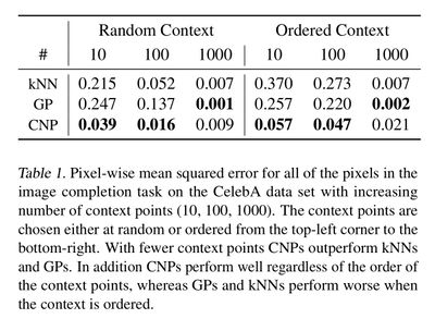
They compared CNPs quantitatively to two related models:
kNNs and GPs. As shown in the above table CNPs outperform
the latter when number of context points is small (empirically
when half of the image or less is provided as context).
When the majority of the image is given as context exact
methods like GPs and kNN will perform better. From the table
we can also see that the order in which the context points
are provided is less important for CNPs, since providing the
context points in order from top to bottom still results in
good performance. Both insights point to the fact that CNPs
learn a data-specific ‘prior’ that will generate good samples
even when the number of context points is very small.
Experimental Result IV: Classification
Finally, they applied the model to one-shot classification using the Omniglot dataset. This dataset consists of 1,623 classes of characters from 50 different alphabets. Each class has only 20 examples and as such this dataset is particularly suitable for few-shot learning algorithms. They used 1,200 randomly selected classes as their training set and the remainder as our testing data set. This includes cropping the image from 32 × 32 to 28 × 28, applying small random translations and rotations to the inputs, and also increasing the number of classes by rotating every character by 90 degrees and defining that to be a new class. They generated the labels for an N-way classification task by choosing N random classes at each training step and arbitrarily assigning the labels 0, ..., N − 1 to each.
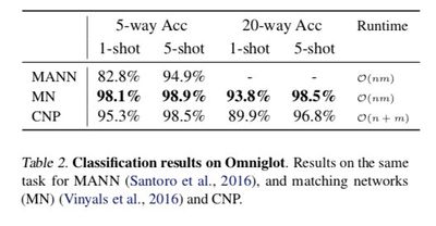
Given that the input points are images, they modified the architecture of the encoder h to include convolution layers as mentioned in section 2. In addition they only aggregated over inputs of the same class by using the information provided by the input label. The aggregated class-specific representations are then concatenated to form the final representation. Given that both the size of the class-specific representations and the number of classes are constant, the size of the final representation is still constant and thus the O(n + m) runtime still holds. The results of the classification are summarized in the following table CNPs achieve higher accuracy than models that are significantly more complex (like MANN). While CNPs do not beat state of the art for one-shot classification our accuracy values are comparable. Crucially, they reached those values using a significantly simpler architecture (three convolutional layers for the encoder and a three-layer MLP for the decoder) and with a lower runtime of O(n + m) at test time as opposed to O(nm)
Conclusion
In this paper they had introduced Conditional Neural Processes, a model that is both flexible at test time and has the capacity to extract prior knowledge from training data.
We had demonstrated its ability to perform a variety of tasks including regression, classification and image completion. We compared CNPs to Gaussian Processes on one hand, and deep learning methods on the other, and also discussed the relation to meta-learning and few-shot learning. It is important to note that the specific CNP implementations described here are just simple proofs-of-concept and can be substantially extended, e.g. by including more elaborate architectures in line with modern deep learning advances. To summarize, this work can be seen as a step towards learning high-level abstractions, one of the grand challenges of contemporary machine learning. Functions learned by most Conditional Neural Processes conventional deep learning models are tied to a specific, constrained statistical context at any stage of training. A trained CNP is more general, in that it encapsulates the high-level statistics of a family of functions. As such it constitutes a high-level abstraction that can be reused for multiple tasks. In future work they are going to explore how far these models can help in tackling the many key machine learning problems that seem to hinge on abstraction, such as transfer learning, meta-learning, and data efficiency.
Reference
Bartunov, S. and Vetrov, D. P. Fast adaptation in generative models with generative matching networks. arXiv preprint arXiv:1612.02192, 2016.
Blundell, C., Cornebise, J., Kavukcuoglu, K., and Wierstra, D. Weight uncertainty in neural networks. arXiv preprint arXiv:1505.05424, 2015.
Bornschein, J., Mnih, A., Zoran, D., and J. Rezende, D. Variational memory addressing in generative models. In Advances in Neural Information Processing Systems, pp. 3923–3932, 2017.
Damianou, A. and Lawrence, N. Deep gaussian processes. In Artificial Intelligence and Statistics, pp. 207–215, 2013.
Devlin, J., Bunel, R. R., Singh, R., Hausknecht, M., and Kohli, P. Neural program meta-induction. In Advances in Neural Information Processing Systems, pp. 2077–2085, 2017.
Edwards, H. and Storkey, A. Towards a neural statistician. 2016.
Finn, C., Abbeel, P., and Levine, S. Model-agnostic metalearning for fast adaptation of deep networks. arXiv preprint arXiv:1703.03400, 2017.
Gal, Y. and Ghahramani, Z. Dropout as a bayesian approximation: Representing model uncertainty in deep learning. In international conference on machine learning, pp. 1050–1059, 2016.
Garnelo, M., Arulkumaran, K., and Shanahan, M. Towards deep symbolic reinforcement learning. arXiv preprint arXiv:1609.05518, 2016.
Gregor, K., Danihelka, I., Graves, A., Rezende, D. J., and Wierstra, D. Draw: A recurrent neural network for image generation. arXiv preprint arXiv:1502.04623, 2015.
Hewitt, L., Gane, A., Jaakkola, T., and Tenenbaum, J. B. The variational homoencoder: Learning to infer high-capacity generative models from few examples. 2018.
J. Rezende, D., Danihelka, I., Gregor, K., Wierstra, D., et al. One-shot generalization in deep generative models. In International Conference on Machine Learning, pp. 1521–1529, 2016.
Kingma, D. P. and Ba, J. Adam: A method for stochastic optimization. arXiv preprint arXiv:1412.6980, 2014.
Kingma, D. P. and Welling, M. Auto-encoding variational bayes. arXiv preprint arXiv:1312.6114, 2013.
Koch, G., Zemel, R., and Salakhutdinov, R. Siamese neural networks for one-shot image recognition. In ICML Deep Learning Workshop, volume 2, 2015.
Lake, B. M., Salakhutdinov, R., and Tenenbaum, J. B. Human-level concept learning through probabilistic program induction. Science, 350(6266):1332–1338, 2015.
Lake, B. M., Ullman, T. D., Tenenbaum, J. B., and Gershman, S. J. Building machines that learn and think like people. Behavioral and Brain Sciences, 40, 2017.
LeCun, Y., Bottou, L., Bengio, Y., and Haffner, P. Gradientbased learning applied to document recognition. Proceedings of the IEEE, 86(11):2278–2324, 1998.
Liu, Z., Luo, P., Wang, X., and Tang, X. Deep learning face attributes in the wild. In Proceedings of International Conference on Computer Vision (ICCV), December 2015.
Louizos, C. and Welling, M. Multiplicative normalizing flows for variational bayesian neural networks. arXiv preprint arXiv:1703.01961, 2017.
Louizos, C., Ullrich, K., and Welling, M. Bayesian compression for deep learning. In Advances in Neural Information Processing Systems, pp. 3290–3300, 2017.
Rasmussen, C. E. and Williams, C. K. Gaussian processes in machine learning. In Advanced lectures on machine learning, pp. 63–71. Springer, 2004.
Reed, S., Chen, Y., Paine, T., Oord, A. v. d., Eslami, S., J. Rezende, D., Vinyals, O., and de Freitas, N. Few-shot autoregressive density estimation: Towards learning to learn distributions. 2017.
Rezende, D. J., Mohamed, S., and Wierstra, D. Stochastic backpropagation and approximate inference in deep generative models. arXiv preprint arXiv:1401.4082, 2014.
Salimbeni, H. and Deisenroth, M. Doubly stochastic variational inference for deep gaussian processes. In Advances in Neural Information Processing Systems, pp. 4591–4602, 2017.
Santoro, A., Bartunov, S., Botvinick, M., Wierstra, D., and Lillicrap, T. One-shot learning with memory-augmented neural networks. arXiv preprint arXiv:1605.06065, 2016.
Snell, J., Swersky, K., and Zemel, R. Prototypical networks for few-shot learning. In Advances in Neural Information Processing Systems, pp. 4080–4090, 2017.
Snelson, E. and Ghahramani, Z. Sparse gaussian processes using pseudo-inputs. In Advances in neural information processing systems, pp. 1257–1264, 2006.
van den Oord, A., Kalchbrenner, N., Espeholt, L., Vinyals, O., Graves, A., et al. Conditional image generation with pixelcnn decoders. In Advances in Neural Information Processing Systems, pp. 4790–4798, 2016.
Vinyals, O., Blundell, C., Lillicrap, T., Wierstra, D., et al. Matching networks for one shot learning. In Advances in Neural Information Processing Systems, pp. 3630–3638, 2016.
Wang, J. X., Kurth-Nelson, Z., Tirumala, D., Soyer, H., Leibo, J. Z., Munos, R., Blundell, C., Kumaran, D., and Botvinick, M. Learning to reinforcement learn. arXiv preprint arXiv:1611.05763, 2016.
Wilson, A. G., Hu, Z., Salakhutdinov, R., and Xing, E. P. Deep kernel learning. In Artificial Intelligence and Statistics, pp. 370–378, 2016.