conditional neural process

Introduction

To train a model effectively, deep neural networks require large datasets. To mitigate this data efficiency problem, learning in two phases is one approach : the first phase learns the statistics of a generic domain without committing to a specific learning task; the second phase learns a function for a specific task, but does so using only a small number of data points by exploiting the domain-wide statistics already learned.

In their work, they proposed a family of models that represent solutions to the supervised problem, and ab end-to-end training approach to learning them, that combine neural networks with features reminiscent if Gaussian Process. They call this family of models Conditional Neural Processes.

Model

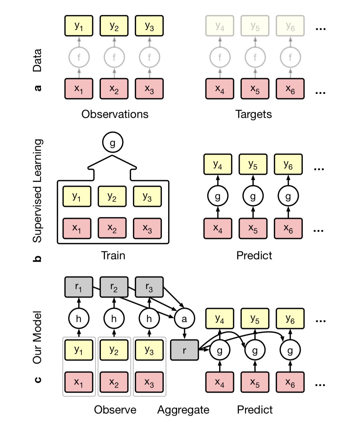
Consider a data set [math]\displaystyle{ \{x_i, y_i\} }[/math] with evaluations [math]\displaystyle{ y_i = f(x_i) }[/math] for some unknown function [math]\displaystyle{ f }[/math]. Assume [math]\displaystyle{ g }[/math] is an approximating function of f. The aim is yo minimize the loss between [math]\displaystyle{ f }[/math] and [math]\displaystyle{ g }[/math] on the entire space [math]\displaystyle{ X }[/math]. In practice, the routine is evaluated on a finite set of observations.

Let training set be [math]\displaystyle{ O = \{x_i, y_i\}_{i = 0} ^ n-1 }[/math], and test set be [math]\displaystyle{ T = \{x_i, y_i\}_{i = n} ^ {n + m - 1} }[/math].

P be a probability distribution over functions [math]\displaystyle{ F : X \to Y }[/math], formally known as a stochastic process. Thus, P defines a joint distribution over the random variables [math]\displaystyle{ {f(x_i)}_{i = 0} ^{n + m - 1} }[/math]. Therefore, for [math]\displaystyle{ P(f(x)|O, T) }[/math], our task is to predict the output values [math]\displaystyle{ f(x_i) }[/math] for [math]\displaystyle{ x_i \in T }[/math], given [math]\displaystyle{ O }[/math],

Conditional Neural Process

Conditional Neural Process models directly parametrize conditional stochastic processes without imposing consistency with respect to some prior process. CNP parametrize distributions over [math]\displaystyle{ f(T) }[/math] given a distributed representation of [math]\displaystyle{ O }[/math] of fixed dimensionality. Thus, the mathematical guarantees associated with stochastic processes is traded off for functional flexibility and scalability.

CNP is a conditional stochastic process [math]\displaystyle{ Q_\theta }[/math] defines distributions over [math]\displaystyle{ f(x_i) }[/math] for [math]\displaystyle{ x_i \in T }[/math]. For stochastic processs, we assume [math]\displaystyle{ Q_theta }[/math] is invariant to permutations, and in this work, we generally enforce permutation invariance with respect to [math]\displaystyle{ T }[/math] be assuming a factored structure. That is, [math]\displaystyle{ Q_theta(f(T) | O, T) = \prod _{x \in T} Q_\theta(f(x) | O, x) }[/math]

In detail, we use the following archiecture

[math]\displaystyle{ r_i = h_\theta(x_i, y_i) }[/math] for any [math]\displaystyle{ (x_i, y_i) \in O }[/math], where [math]\displaystyle{ h_\theta : X \times Y \to \mathbb{R} ^ d }[/math]

[math]\displaystyle{ r = r_i * r_2 * ... * r_n }[/math], where [math]\displaystyle{ * }[/math] is a commutative operation that takes elements in [math]\displaystyle{ \mathbb{R}^d }[/math] and maps them into a single element of [math]\displaystyle{ \mathbb{R} ^ d }[/math]

[math]\displaystyle{ \Phi_i = g_\theta }[/math] for any [math]\displaystyle{ x_i \in T }[/math], where [math]\displaystyle{ g_\theta : X \times \mathbb{R} ^ d \to \mathbb{R} ^ e }[/math] and [math]\displaystyle{ \Phi_i }[/math] are parameters for [math]\displaystyle{ Q_\theta }[/math]

Note that this architecture ensures permutation invariance and [math]\displaystyle{ O(n + m) }[/math] scaling for conditional prediction. Also, [math]\displaystyle{ r = r_i * r_2 * ... * r_n }[/math] can be computed in [math]\displaystyle{ O(n) }[/math], this architecture supports streaming observation with minimal overhead.

We train [math]\displaystyle{ Q_\theta }[/math] by asking it to predict [math]\displaystyle{ O }[/math] conditioned on a randomly chosen subset of [math]\displaystyle{ O }[/math]. This gives the model a signal of the uncertainty over the space X inherent in the distribution P given a set of observations. Thus, the targets it scores [math]\displaystyle{ Q_\theta }[/math] on include both the observed and unobserved values. In practice, we take Monte Carlo estimates of the gradient of this loss by sampling [math]\displaystyle{ f }[/math] and [math]\displaystyle{ N }[/math]. This approach shifts the burden of imposing prior knowledge

from an analytic prior to empirical data. This has the advantage of liberating a practitioner from having to specify an analytic form for the prior, which is ultimately intended to summarize their empirical experience. Still, we emphasize that the [math]\displaystyle{ Q_\theta }[/math] are not necessarily a consistent set of conditionals for all observation sets, and the training routine does not guarantee that.

In summary,

1. A CNP is a conditional distribution over functions trained to model the empirical conditional distributions of functions [math]\displaystyle{ f \sim P }[/math].

2. A CNP is permutation invariant in [math]\displaystyle{ O }[/math] and [math]\displaystyle{ T }[/math].

3. A CNP is scalable, achieving a running time complexity of [math]\displaystyle{ O(n + m) }[/math] for making [math]\displaystyle{ m }[/math] predictions with [math]\displaystyle{ n }[/math] observations.

Experimental Result I: Function Regression

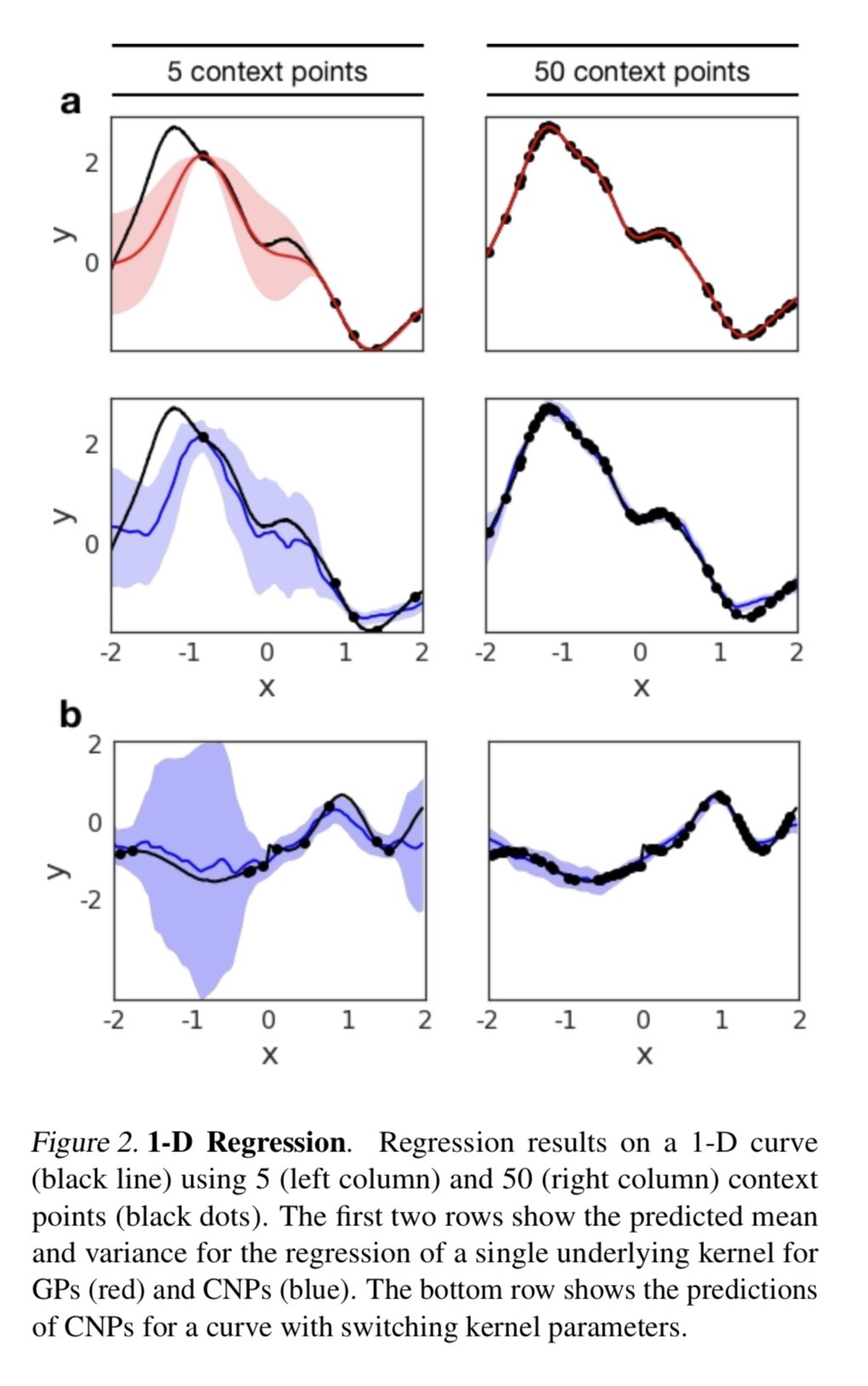
Classical 1D regression task that used as a common baseline for GP is our first example. They generated two different datasets that consisted of functions generated from a GP with an exponential kernel. In the first dataset they used a kernel with fixed parameters, and in the second dataset the function switched at some random point. on the real line between two functions each sampled with different kernel parameters. At every training step they sampled a curve from the GP, select a subset of n points as observations, and a subset of t points as target points. Using the model, the observed points are encoded using a three layer MLP encoder h with a 128 dimensional output representation. The representations are aggregated into a single representation [math]\displaystyle{ r = \frac{1}{n} \sum r_i }[/math] , which is concatenated to [math]\displaystyle{ x_t }[/math] and passed to a decoder g consisting of a five layer MLP.

Two examples of the regression results obtained for each of the datasets are shown in the following figure.

They compared the model to the predictions generated by a GP with the correct hyperparameters, which constitutes an upper bound on our performance. Although the prediction generated by the GP is smoother than the CNP's prediction both for the mean and variance, the model is able to learn to regress from a few context points for both the fixed kernels and switching kernels. As the number of context points grows, the accuracy of the model improves and the approximated uncertainty of the model decreases. Crucially, we see the model learns to estimate its own uncertainty given the observations very accurately. Nonetheless it provides a good approximation that increases in accuracy as the number of context points increases. Furthermore the model achieves similarly good performance on the switching kernel task. This type of regression task is not trivial for GPs whereas in our case we only have to change the dataset used for training

Experimental Result II: Image Completion for Digits

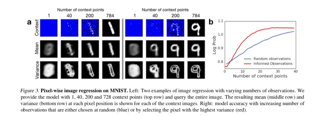
They also tested CNP on the MNIST dataset and use the test set to evaluate its performance. As shown in the above figure the model learns to make good predictions of the underlying digit even for a small number of context points. Crucially, when conditioned only on one non-informative context point the model’s prediction corresponds to the average over all MNIST digits. As the number of context points increases the predictions become more similar to the underlying ground truth. This demonstrates the model’s capacity to extract dataset specific prior knowledge. It is worth mentioning that even with a complete set of observations the model does not achieve pixel-perfect reconstruction, as we have a bottleneck at the representation level. Since this implementation of CNP returns factored outputs, the best prediction it can produce given limited context information is to average over all possible predictions that agree with the context. An alternative to this is to add latent variables in the model such that they can be sampled conditioned on the context to produce predictions with high probability in the data distribution.

An important aspect of the model is its ability to estimate the uncertainty of the prediction. As shown in the bottom row of the above figure, as they added more observations, the variance shifts from being almost uniformly spread over the digit positions to being localized around areas that are specific to the underlying digit, specifically its edges. Being able to model the uncertainty given some context can be helpful for many tasks. One example is active exploration, where the model has a choice over where to observe. They tested this by comparing the predictions of CNP when the observations are chosen according to uncertainty, versus random pixels. This method is a very simple way of doing active exploration, but it already produces better prediction results than selecting the conditioning points at random.