continuous space language models: Difference between revisions
No edit summary |
|||
| Line 11: | Line 11: | ||
Let H be the weight matrix from the projection layer to the hidden layer and the state of H would be: | Let H be the weight matrix from the projection layer to the hidden layer and the state of H would be: | ||
[[File:Qq.png]] | |||
<math>\,h=tanh(Ha + b)</math> where A is the concatenation of all <math>\,a_i</math> and <math>\,b</math> is some bias vector | <math>\,h=tanh(Ha + b)</math> where A is the concatenation of all <math>\,a_i</math> and <math>\,b</math> is some bias vector | ||
Finally, the output vector would be: | Finally, the output vector would be: | ||
<math>\,o=Vh+k</math> where V is the weight matrix from hidden to output and k is another bias vector. <math>\,o</math> would be a vector with same dimensions as the total vocabulary size and the probabilities can be | <math>\,o=Vh+k</math> where V is the weight matrix from hidden to output and k is another bias vector. <math>\,o</math> would be a vector with same dimensions as the total vocabulary size and the probabilities can be cal[[File:Q3.png]]culated from <math>\,o</math> by applying the softmax function. | ||
The following figure shows the Architecture of the neural network language model. <math>\,h_j</math> denotes the context <math>\,w_{j-n+1}^{j-1}</math>. P is the size of one projection and H and N is the | The following figure shows the Architecture of the neural network language model. <math>\,h_j</math> denotes the context <math>\,w_{j-n+1}^{j-1}</math>. P is the size of one projection and H and N is the | ||
Revision as of 19:04, 12 December 2015
Model
The neural network language model has to perform two tasks: first, project all words of the context [math]\displaystyle{ \,h_j }[/math] = [math]\displaystyle{ \,w_{j-n+1}^{j-1} }[/math] onto a continuous space, and second, calculate the language model probability [math]\displaystyle{ P(w_{j}=i|h_{j}) }[/math]. The researchers for this paper sought to find a better model for this probability than the back-off n-grams model. Their approach was to map the n-1 words sequence onto a multi-dimension continuous space using a layer of neural network followed by another layer to estimate the probabilities of all possible next words. The formulas and model goes as follows:
For some sequence of n-1 words, encode each word using 1 of K encoding, i.e. 1 where the word is indexed and zero everywhere else. Label each 1 of K encoding by [math]\displaystyle{ (w_{j-n+1},\dots,w_j) }[/math] for some n-1 word sequence at the j'th word in some larger context.
Let P be a projection matrix common to all n-1 words and let
[math]\displaystyle{ \,a_i=Pw_{j-n+i},i=1,\dots,n-1 }[/math]
Let H be the weight matrix from the projection layer to the hidden layer and the state of H would be: File:Qq.png [math]\displaystyle{ \,h=tanh(Ha + b) }[/math] where A is the concatenation of all [math]\displaystyle{ \,a_i }[/math] and [math]\displaystyle{ \,b }[/math] is some bias vector
Finally, the output vector would be:
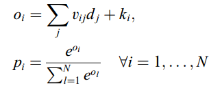
[math]\displaystyle{ \,o=Vh+k }[/math] where V is the weight matrix from hidden to output and k is another bias vector. [math]\displaystyle{ \,o }[/math] would be a vector with same dimensions as the total vocabulary size and the probabilities can be cal culated from [math]\displaystyle{ \,o }[/math] by applying the softmax function.
The following figure shows the Architecture of the neural network language model. [math]\displaystyle{ \,h_j }[/math] denotes the context [math]\displaystyle{ \,w_{j-n+1}^{j-1} }[/math]. P is the size of one projection and H and N is the size of the second hidden and output layer, respectively. When short-lists are used the size of the output layer is much smaller than the size of the vocabulary.
In contrast to standard languaFile:Qq.pngge modeling where we want to know the probability of a word i given its context, [math]\displaystyle{ P(w_{j} = i|h_{j}) }[/math], the neural network simultaneously predicts the language model probability of all words in the word list:
