Neural ODEs: Difference between revisions
m (→Implementation) |
m (→Implementation) |
||
| Line 81: | Line 81: | ||
===Implementation=== | ===Implementation=== | ||
The authors construct two separate types of neural networks to compare against each other, the first is the standard planar Normalizing Flow network (NF) using 64 layers of single hidden units, and the second is their new CNF with 64 hidden units. The NF model is trained over 500,000 iterations using RMSprop, and the CNF network is trained over 10,000 iterations using Adam. The loss function is <math>KL(q(x)||p(x))</math> where <math>q(x)</math> is the flow model and <math>p(x)</math> is the target probability density. | The authors construct two separate types of neural networks to compare against each other, the first is the standard planar Normalizing Flow network (NF) using 64 layers of single hidden units, and the second is their new CNF with 64 hidden units. The NF model is trained over 500,000 iterations using RMSprop, and the CNF network is trained over 10,000 iterations using Adam(algorithm for first-order gradient-based optimization of stochastic objective functions). The loss function is <math>KL(q(x)||p(x))</math> where <math>q(x)</math> is the flow model and <math>p(x)</math> is the target probability density. | ||
One of the biggest advantages when implementing CNF is that you can train the flow parameters just by performing maximum likelihood estimation on <math>\log(q(x))</math> given <math>p(x)</math>, where <math>q(x)</math> is found via the theorem above, and then reversing the CNF to generate random samples from <math>q(x)</math>. This reversal of the CNF is done with about the same cost of the forward pass which is not able to be done in an NF network. The following two figures demonstrate the ability of CNF to generate more expressive and accurate output data as compared to standard NF networks. | One of the biggest advantages when implementing CNF is that you can train the flow parameters just by performing maximum likelihood estimation on <math>\log(q(x))</math> given <math>p(x)</math>, where <math>q(x)</math> is found via the theorem above, and then reversing the CNF to generate random samples from <math>q(x)</math>. This reversal of the CNF is done with about the same cost of the forward pass which is not able to be done in an NF network. The following two figures demonstrate the ability of CNF to generate more expressive and accurate output data as compared to standard NF networks. | ||
Revision as of 23:50, 23 November 2020
Introduction
Chen et al. propose a new class of neural networks called neural ordinary differential equations (ODEs) in their 2018 paper under the same title. Neural network models, such as residual or recurrent networks, can be generalized as a set of transformations through hidden states (a.k.a layers) [math]\displaystyle{ \mathbf{h} }[/math], given by the equation
where [math]\displaystyle{ t \in \{0,...,T\} }[/math] and [math]\displaystyle{ \theta_t }[/math] corresponds to the set of parameters or weights in state [math]\displaystyle{ t }[/math]. It is important to note that it has been shown (Lu et al., 2017)(Haber and Ruthotto, 2017)(Ruthotto and Haber, 2018) that Equation 1 can be viewed as an Euler discretization. Given this Euler description, if the number of layers and step size between layers are taken to their limits, then Equation 1 can instead be described continuously in the form of the ODE,
Equation 2 now describes a network where the output layer [math]\displaystyle{ \mathbf{h}(T) }[/math] is generated by solving for the ODE at time [math]\displaystyle{ T }[/math], given the initial value at [math]\displaystyle{ t=0 }[/math], where [math]\displaystyle{ \mathbf{h}(0) }[/math] is the input layer of the network.
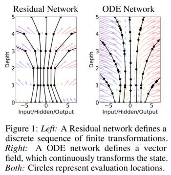
With a vast amount of theory and research in the field of solving ODEs numerically, there are a number of benefits to formulating the hidden state dynamics this way. One major advantage is that a continuous description of the network allows for the calculation of [math]\displaystyle{ f }[/math] at arbitrary intervals and locations. The authors provide an example in section five of how the neural ODE network outperforms the discretized version i.e. residual networks, by taking advantage of the continuity of [math]\displaystyle{ f }[/math]. A depiction of this distinction is shown in the figure below.
In section four the authors show that the single-unit bottleneck of normalizing flows can be overcome by constructing a new class of density models that incorporates the neural ODE network formulation. The next section on automatic differentiation will describe how utilizing ODE solvers allows for the calculation of gradients of the loss function without storing any of the hidden state information. This results in a very low memory requirement for neural ODE networks in comparison to traditional networks that rely on intermediate hidden state quantities for backpropagation.
Reverse-mode Automatic Differentiation of ODE Solutions
Like most neural networks, optimizing the weight parameters [math]\displaystyle{ \theta }[/math] for a neural ODE network involves finding the gradient of a loss function with respect to those parameters. Differentiating in the forward direction is a simple task, however, this method is very computationally expensive and unstable, as it introduces additional numerical error. Instead, the authors suggest that the gradients can be calculated in the reverse-mode with the adjoint sensitivity method (Pontryagin et al., 1962). This "backpropagation" method solves an augmented version of the forward ODE problem but in reverse, which is something that all ODE solvers are capable of. Section 3 provides results showing that this method gives very desirable memory costs and numerical stability.
The authors provide an example of the adjoint method by considering the minimization of the scalar-valued loss function [math]\displaystyle{ L }[/math], which takes the solution of the ODE solver as its argument.
This minimization problem requires the calculation of [math]\displaystyle{ \frac{\partial L}{\partial \mathbf{z}(t_0)} }[/math] and [math]\displaystyle{ \frac{\partial L}{\partial \theta} }[/math].
The adjoint itself is defined as [math]\displaystyle{ \mathbf{a}(t) = \frac{\partial L}{\partial \mathbf{z}(t)} }[/math], which describes the gradient of the loss with respect to the hidden state [math]\displaystyle{ \mathbf{z}(t) }[/math]. By taking the first derivative of the adjoint, another ODE arises in the form of,
Since the value [math]\displaystyle{ \mathbf{a}(t_0) }[/math] is required to minimize the loss, the ODE in equation 3 must be solved backwards in time from [math]\displaystyle{ \mathbf{a}(t_1) }[/math]. Solving this problem is dependent on the knowledge of the hidden state [math]\displaystyle{ \mathbf{z}(t) }[/math] for all [math]\displaystyle{ t }[/math], which an neural ODE does not save on the forward pass. Luckily, both [math]\displaystyle{ \mathbf{a}(t) }[/math] and [math]\displaystyle{ \mathbf{z}(t) }[/math] can be calculated in reverse, at the same time, by setting up an augmented version of the dynamics and is shown in the final algorithm. Finally, the derivative [math]\displaystyle{ dL/d\theta }[/math] can be expressed in terms of the adjoint and the hidden state as,
To obtain very inexpensive calculations of [math]\displaystyle{ \frac{\partial f}{\partial z} }[/math] and [math]\displaystyle{ \frac{\partial f}{\partial \theta} }[/math] in equation 3 and 4, automatic differentiation can be utilized. The authors present an algorithm to calculate the gradients of [math]\displaystyle{ L }[/math] and their dependent quantities with only one call to an ODE solver and is shown below.
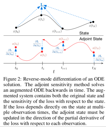
If the loss function has a stronger dependence on the hidden states for [math]\displaystyle{ t \neq t_0,t_1 }[/math], then Algorithm 1 can be modified to handle multiple calls to the ODESolve step since most ODE solvers have the capability to provide [math]\displaystyle{ z(t) }[/math] at arbitrary times. A visual depiction of this scenario is shown below.
Please see the appendix for extended versions of Algorithm 1 and detailed derivations of each equation in this section.
Replacing Residual Networks with ODEs for Supervised Learning
Section three of the paper investigates an application of the reverse-mode differentiation described in section two, for the training of neural ODE networks on the MNIST digit data set. To solve for the forward pass in the neural ODE network, the following experiment used Adams method, which is an implicit ODE solver. Although it has a marked improvement over explicit ODE solvers in numerical accuracy, integrating backward through the network for backpropagation is still not preferred and the adjoint sensitivity method is used to perform efficient weight optimization. The network with this "backpropagation" technique is referred to as ODE-Net in this section.
Implementation
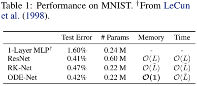
A residual network (ResNet), studied by He et al. (2016), with six standard residual blocks was used as a comparative model for this experiment. The competing model, ODE-net, replaces the residual blocks of the ResNet with the Adams solver. As a hybrid of the two models ResNet and ODE-net, a third network was created called RK-Net, which solves the weight optimization of the neural ODE network explicitly through backward Runge-Kutta integration. The following table shows the training and performance results of each network.
Note that [math]\displaystyle{ L }[/math] and [math]\displaystyle{ \tilde{L} }[/math] are the number of layers in ResNet and the number of function calls that the Adams method makes for the two ODE networks and are effectively analogous quantities. As shown in Table 1, both of the ODE networks achieve comparable performance to that of the ResNet with a notable decrease in memory cost for ODE-net.
Another interesting component of ODE networks is the ability to control the tolerance in the ODE solver used and subsequently the numerical error in the solution.
The tolerance of the ODE solver is represented by the colour bar in Figure 3 above and notice that a variety of effects arise from adjusting this parameter. Primarily, if one was to treat the tolerance as a hyperparameter of sorts, you could tune it such that you find a balance between accuracy (Figure 3a) and computational complexity (Figure 3b). Figure 3c also provides further evidence for the benefits of the adjoint method for the backward pass in ODE-nets since there is a nearly 1:0.5 ratio of forward to backward function calls. In the ResNet and RK-Net examples, this ratio is 1:1.
Additionally, the authors loosely define the concept of depth in a neural ODE network by referring to Figure 3d. Here it's evident that as you continue to train an ODE network, the number of function evaluations the ODE solver performs increases. As previously mentioned, this quantity is comparable to the network depth of a discretized network. However, as the authors note, this result should be seen as the progression of the network's complexity over training epochs, which is something we expect to increase over time.
Continuous Normalizing Flows
Section four tackles the implementation of continuous-depth Neural Networks, but to do so, in the first part of section four the authors discuss theoretically how to establish this kind of network through the use of normalizing flows. The authors use a change of variables method presented in other works (Rezende and Mohamed, 2015), (Dinh et al., 2014), to compute the change of a probability distribution if sample points are transformed through a bijective function, [math]\displaystyle{ f }[/math].
Where p(z) is the probability distribution of the samples and [math]\displaystyle{ det\frac{\partial f}{\partial z_0} }[/math] is the determinant of the Jacobian which has a cubic cost in the dimension of z or the number of hidden units in the network. The authors discovered however that transforming the discrete set of hidden layers in the normalizing flow network to continuous transformations simplifies the computations significantly, due primarily to the following theorem:
Theorem 1: (Instantaneous Change of Variables). Let z(t) be a finite continuous random variable with probability p(z(t)) dependent on time. Let dz/dt=f(z(t),t) be a differential equation describing a continuous-in-time transformation of z(t). Assuming that f is uniformly Lipschitz continuous in z and continuous in t, then the change in log probability also follows a differential equation:
The biggest advantage to using this theorem is that the trace function is a linear function, so if the dynamics of the problem, f, is represented by a sum of functions, then so is the log density. This essentially means that you can now compute flow models with only a linear cost with respect to the number of hidden units, [math]\displaystyle{ M }[/math]. In standard normalizing flow models, the cost is [math]\displaystyle{ O(M^3) }[/math], so they will generally fit many layers with a single hidden unit in each layer.
Finally the authors use these realizations to construct Continuous Normalizing Flow networks (CNFs) by specifying the parameters of the flow as a function of t, ie, [math]\displaystyle{ f(z(t),t) }[/math]. They also use a gating mechanism for each hidden unit, [math]\displaystyle{ \frac{dz}{dt}=\sum_n \sigma_n(t)f_n(z) }[/math] where [math]\displaystyle{ \sigma_n(t)\in (0,1) }[/math] is a separate neural network which learns when to apply each dynamic [math]\displaystyle{ f_n }[/math].
Implementation
The authors construct two separate types of neural networks to compare against each other, the first is the standard planar Normalizing Flow network (NF) using 64 layers of single hidden units, and the second is their new CNF with 64 hidden units. The NF model is trained over 500,000 iterations using RMSprop, and the CNF network is trained over 10,000 iterations using Adam(algorithm for first-order gradient-based optimization of stochastic objective functions). The loss function is [math]\displaystyle{ KL(q(x)||p(x)) }[/math] where [math]\displaystyle{ q(x) }[/math] is the flow model and [math]\displaystyle{ p(x) }[/math] is the target probability density.
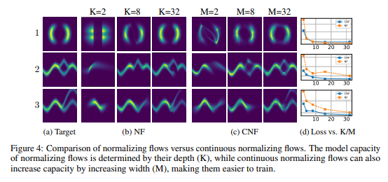
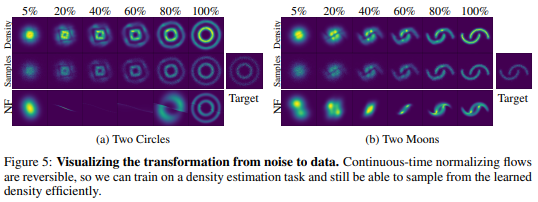
One of the biggest advantages when implementing CNF is that you can train the flow parameters just by performing maximum likelihood estimation on [math]\displaystyle{ \log(q(x)) }[/math] given [math]\displaystyle{ p(x) }[/math], where [math]\displaystyle{ q(x) }[/math] is found via the theorem above, and then reversing the CNF to generate random samples from [math]\displaystyle{ q(x) }[/math]. This reversal of the CNF is done with about the same cost of the forward pass which is not able to be done in an NF network. The following two figures demonstrate the ability of CNF to generate more expressive and accurate output data as compared to standard NF networks.
Figure 4 shows clearly that the CNF structure exhibits significantly lower loss functions than NF. In figure 5 both networks were tasked with transforming a standard Gaussian distribution into a target distribution, not only was the CNF network more accurate on the two moons target, but also the steps it took along the way are much more intuitive than the output from NF.
A Generative Latent Function Time-Series Model
One of the largest issues at play in terms of Neural ODE networks is the fact that in many instances, data points are either very sparsely distributed, or irregularly-sampled. The latent dynamics are discretized and the observations are in the bins of fixed duration. An example of this is medical records which are only updated when a patient visits a doctor or the hospital. To solve this issue the authors had to create a generative time-series model which would be able to fill in the gaps of missing data. The authors consider each time series as a latent trajectory stemming from the initial local state [math]\displaystyle{ z_{t_0 } }[/math] and determined from a global set of latent parameters. Given a set of observation times and initial state, the generative model constructs points via the following sample procedure:
[math]\displaystyle{ z_{t_0}∼p(z_{t_0}) }[/math]
[math]\displaystyle{ z_{t_1},z_{t_2},\dots,z_{t_N}={\rm ODESolve}(z_{t_0},f,θ_f,t_0,...,t_N) }[/math]
each [math]\displaystyle{ x_{t_i}∼p(x│z_{t_i},θ_x) }[/math]
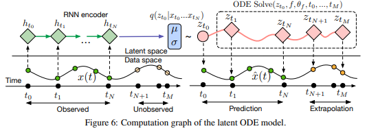
[math]\displaystyle{ f }[/math] is a function which outputs the gradient [math]\displaystyle{ \frac{\partial z(t)}{\partial t}=f(z(t),θ_f) }[/math] which is parameterized via a neural net. In order to train this latent variable model, the authors had to first encode their given data and observation times using an RNN encoder, construct the new points using the trained parameters, then decode the points back into the original space. The following figure describes this process:
Another variable which could affect the latent state of a time-series model is how often an event actually occurs. The authors solved this by parameterizing the rate of events in terms of a Poisson process. They described the set of independent observation times in an interval [math]\displaystyle{ \left[t_{start},t_{end}\right] }[/math] as:
[math]\displaystyle{ {\rm log}(p(t_1,t_2,\dots,t_N ))=\sum_{i=1}^N{\rm log}(\lambda(z(t_i)))-\int_{t_{start}}^{t_{end}}λ(z(t))dt }[/math]
where [math]\displaystyle{ \lambda(*) }[/math] is parameterized via another neural network.
Implementation
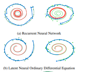
To test the effectiveness of the Latent time-series ODE model (LODE), they fit the encoder with 25 hidden units, parametrize function f with a one-layer 20 hidden unit network, and the decoder as another neural network with 20 hidden units. They compare this against a standard recurrent neural net (RNN) with 25 hidden units trained to minimize Gaussian log-likelihood. The authors tested both of these network systems on a dataset of 2-dimensional spirals which either rotated clockwise or counter-clockwise and sampled the positions of each spiral at 100 equally spaced time steps. They can then simulate irregularly timed data by taking random amounts of points without replacement from each spiral. The next two figures show the outcome of these experiments:
In the figure on the right the blue lines represent the test data learned curves and the red lines represent the extrapolated curves predicted by each model. It is noted that the LODE performs significantly better than the standard RNN model, especially on smaller sets of data points.
Scope and Limitations
Section 6 mainly discusses the scope and limitations of the paper. Firstly while “batching” the training data is a useful step in standard neural nets, and can still be applied here by combining the ODEs associated with each batch, the authors found that controlling the error, in this case, may increase the number of calculations required. In practice, however, the number of calculations did not increase significantly.
So long as the model proposed in this paper uses finite weights and Lipschitz nonlinearities, then Picard’s existence theorem (Coddington and Levinson, 1955) applies, guaranteeing the solution to the IVP exists and is unique. This theorem holds for the model presented above when the network has finite weights and uses nonlinearities in the Lipshitz class.
In controlling the amount of error in the model, the authors were only able to reduce tolerances to approximately [math]\displaystyle{ 10^{-3} }[/math] and [math]\displaystyle{ 10^{-5} }[/math] in classification and density estimation respectively without also degrading the computational performance.
The authors believe that reconstructing state trajectories by running the dynamics backward can introduce extra numerical error. They address a possible solution to this problem by checkpointing certain time steps and storing intermediate values of z on the forward pass. Then while reconstructing, you do each part individually between checkpoints. The authors acknowledged that they informally checked the validity of this method since they don’t consider it a practical problem.
There remain, however, areas where standard neural networks may perform better than Neural ODEs. Firstly, conventional nets can fit non-homeomorphic functions, for example, functions whose output has a smaller dimension that their input, or that change the topology of the input space. However, this could be handled by composing ODE nets with standard network layers. Another point is that conventional nets can be evaluated exactly with a fixed amount of computation, and are typically faster to train and do not require an error tolerance for a solver.
Conclusions and Critiques
We covered the use of black-box ODE solvers as a model component and their application to initial value problems constructed from real applications. Neural ODE Networks show promising gains in computational cost without large sacrifices in accuracy when applied to certain problems. A drawback of some of these implementations is that the ODE Neural Networks are limited by the underlying distributions of the problems they are trying to solve (requirement of Lipschitz continuity, etc.). There are plenty of further advances to be made in this field as hundreds of years of ODE theory and literature is available, so this is currently an important area of research.
ODEs indeed represent an important area of applied mathematics where neural networks can be used to solve them numerically. Perhaps, a parallel area of investigation can be PDEs (Partial Differential Equations). PDEs are also widely encountered in many areas of applied mathematics, physics, social sciences and many other fields. It will be interesting to see how neural networks can be used to solve PDEs.
More Critiques
This paper covers the memory efficiency of Neural ODE Networks, but does not address runtime. In practice, most systems are bound by latency requirements more-so than memory requirements (except in edge device cases). Though it may be unreasonable to expect the authors to produce a performance-optimized implementation, it would be insightful to understand the computational bottlenecks so existing frameworks can take steps to address them. This model looks promising and practical performance is the key to enabling future research in this.
The above critique also questions the need for a neural network for such a problem. This problem was studied by Brunel et al. and they presented their solution in their paper Parametric Estimation of Ordinary Differential Equations with Orthogonality Conditions. While this solution also requires iteratively solving a complex optimization problem, they did not require the massive memory and runtime overhead of a neural network. For the neural network solution to demonstrate its potential, it should be including experimental comparisons with specialized ordinary differential equation algorithms instead of simply comparing with a general recurrent neural network.
References
Yiping Lu, Aoxiao Zhong, Quanzheng Li, and Bin Dong. Beyond finite layer neural networks: Bridging deep architectures and numerical differential equations. arXiv preprint arXiv:1710.10121, 2017.
Eldad Haber and Lars Ruthotto. Stable architectures for deep neural networks. Inverse Problems, 34 (1):014004, 2017.
Lars Ruthotto and Eldad Haber. Deep neural networks motivated by partial differential equations. arXiv preprint arXiv:1804.04272, 2018.
Lev Semenovich Pontryagin, EF Mishchenko, VG Boltyanskii, and RV Gamkrelidze. The mathematical theory of optimal processes. 1962.
Kaiming He, Xiangyu Zhang, Shaoqing Ren, and Jian Sun. Identity mappings in deep residual networks. In European conference on computer vision, pages 630–645. Springer, 2016b.
Earl A Coddington and Norman Levinson. Theory of ordinary differential equations. Tata McGrawHill Education, 1955.
Danilo Jimenez Rezende and Shakir Mohamed. Variational inference with normalizing flows. arXiv preprint arXiv:1505.05770, 2015.
Laurent Dinh, David Krueger, and Yoshua Bengio. NICE: Non-linear independent components estimation. arXiv preprint arXiv:1410.8516, 2014.
Brunel, N. J., Clairon, Q., & d’Alché-Buc, F. (2014). Parametric estimation of ordinary differential equations with orthogonality conditions. Journal of the American Statistical Association, 109(505), 173-185.
