stat946w18/Rethinking the Smaller-Norm-Less-Informative Assumption in Channel Pruning of Convolutional Layers: Difference between revisions
| Line 78: | Line 78: | ||
== Results == | == Results == | ||
=== CIFAR-10 Experiment === | === CIFAR-10 Experiment === | ||
Revision as of 00:18, 21 April 2018
Introduction
With the recent and ongoing surge in low-power, intelligent agents (such as wearables, smartphones, and IoT devices), there exists a growing need for machine learning models to work well in resource-constrained environments. Deep learning models have achieved state-of-the-art on a broad range of tasks; however, they are difficult to deploy in their original forms. For example, AlexNet (Krizhevsky et al., 2012), a model for image classification, contains 61 million parameters and requires 1.5 billion floating point operations (FLOPs) in one inference pass. A more accurate model, ResNet-50 (He et al., 2016), has 25 million parameters but requires 4.08 FLOPs. A high-end desktop GPU such as a Titan Xp is capable of (12 TFLOPS (tera-FLOPs per second)), while the Adreno 540 GPU used in a Samsung Galaxy S8 is only capable of (567 GFLOPS) which is less than 5% of the Titan Xp. Clearly, it would be difficult to deploy and run these models on low-power devices.
In general, model compression can be accomplished using four main non-mutually exclusive methods (Cheng et al., 2017): weight pruning, quantization, matrix transformations, and weight tying. By non-mutually exclusive, we mean that these methods can be used not only separately but also in combination for compressing a single model; the use of one method does not exclude any of the other methods from being viable.
Ye et al. (2018) explores pruning entire channels in a convolutional neural network (CNN). Past work has mostly focused on norm[based or error-based heuristics to prune channels; instead, Ye et al. (2018) show that their approach is easily reproducible and has favorable qualities from an optimization standpoint. In other words, they argue that the norm-based assumption is not as informative or theoretically justified as their approach, and provide strong empirical evidence of these findings.
Motivation
Some previous works on pruning channel filters (Li et al., 2016; Molchanov et al., 2016) have focused on using the L1 norm to determine the importance of a channel. Ye et al. (2018) show that, in the deep linear convolution case, penalizing the per-layer norm is coarse-grained; they argue that one cannot assign different coefficients to L1 penalties associated with different layers without risking the loss function being susceptible to trivial re-parameterizations. As an example, consider the following deep linear convolutional neural network with modified LASSO loss:
$$\min \mathbb{E}_D \lVert W_{2n} * \dots * W_1 x - y\rVert^2 + \lambda \sum_{i=1}^n \lVert W_{2i} \rVert_1$$
where W are the weights and * is convolution. Here we have chosen the coefficient 0 for the L1 penalty associated with odd-numbered layers and the coefficient 1 for the L1 penalty associated with even-numbered layers. This loss is susceptible to trivial re-parameterizations: without affecting the least-squares loss, we can always reduce the LASSO loss by halving the weights of all even-numbered layers and doubling the weights of all odd-numbered layers.
Furthermore, batch normalization (Ioffe, 2015) is incompatible with this method of weight regularization. Consider batch normalization at the [math]\displaystyle{ l }[/math]-th layer.
Due to the batch normalization, any uniform scaling of [math]\displaystyle{ W^l }[/math] which would change [math]\displaystyle{ l_1 }[/math] and [math]\displaystyle{ l_2 }[/math] norms, but has no have no effect on [math]\displaystyle{ x^{l+1} }[/math]. Thus, when trying to minimize weight norms of multiple layers, it is unclear how to properly choose penalties for each layer. Therefore, penalizing the norm of a filter in a deep convolutional network is hard to justify from a theoretical perspective.
In contrast with these existing approaches, the authors focus on enforcing sparsity of a tiny set of parameters in CNN — scale parameter [math]\displaystyle{ \gamma }[/math] in all batch normalization. Not only placing sparse constraints on [math]\displaystyle{ \gamma }[/math] is simpler and easier to monitor, but more importantly, they put forward two reasons:
1. Every [math]\displaystyle{ \gamma }[/math] always multiplies a normalized random variable, thus the channel importance becomes comparable across different layers by measuring the magnitude values of [math]\displaystyle{ \gamma }[/math];
2. The reparameterization effect across different layers is avoided if its subsequent convolution layer is also batch-normalized. In other words, the impacts from the scale changes of [math]\displaystyle{ \gamma }[/math] parameter are independent across different layers.
Thus, although not providing a complete theoretical guarantee on loss, Ye et al. (2018) develop a pruning technique that claims to be more justified than norm-based pruning is.
Method
At a high level, Ye et al. (2018) propose that, instead of discovering sparsity via penalizing the per-filter or per-channel norm, penalize the batch normalization scale parameters gamma instead. The reasoning is that by having fewer parameters to constrain and working with normalized values, sparsity is easier to enforce, monitor, and learn. Having sparse batch normalization terms has the effect of pruning entire channels: if gamma is zero, then the output at that layer becomes constant (the bias term), and thus the preceding channels can be pruned.
Summary
The basic algorithm can be summarized as follows:
1. Penalize the L1-norm of the batch normalization scaling parameters in the loss
2. Train until loss plateaus
3. Remove channels that correspond to a downstream zero in batch normalization
4. Fine-tune the pruned model using regular learning
Details
There still exist a few problems that this summary has not addressed so far. Sub-gradient descent is known to have inverse square root convergence rate on subdifferentials (Gordon et al., 2012), so the sparsity gradient descent update may be suboptimal. Furthermore, the sparse penalty needs to be normalized with respect to previous channel sizes, since the penalty should be roughly equally distributed across all convolution layers.
Slow Convergence
To address the issue of slow convergence, Ye et al. (2018) use an iterative shrinking-thresholding algorithm (ISTA) (Beck & Teboulle, 2009) to update the batch normalization scale parameter. The intuition for ISTA is that the structure of the optimization objective can be taken advantage of. Consider: $$L(x) = f(x) + g(x).$$
Let f be the model loss and g be the non-differentiable penalty (LASSO). ISTA is able to use the structure of the loss and converge in O(1/n), instead of O(1/sqrt(n)) when using subgradient descent, which assumes no structure about the loss. Even though ISTA is used in convex settings, Ye et. al (2018) argue that it still performs better than gradient descent.
Penalty Normalization
In the paper, Ye et al. (2018) normalize the per-layer sparse penalty with respect to the global input size, the current layer kernel areas, the previous layer kernel areas, and the local input feature map area.
To control the global penalty, a hyperparamter rho is multiplied with all the per-layer lambda in the final loss.
Steps
The final algorithm can be summarized as follows:
1. Compute the per-layer normalized sparse penalty constant [math]\displaystyle{ \lambda }[/math]
2. Compute the global LASSO loss with global scaling constant [math]\displaystyle{ \rho }[/math]
3. Until convergence, train scaling parameters using ISTA and non-scaling parameters using regular gradient descent.
4. Remove channels that correspond to a downstream zero in batch normalization
5. Fine-tune the pruned model using regular learning
Results
CIFAR-10 Experiment
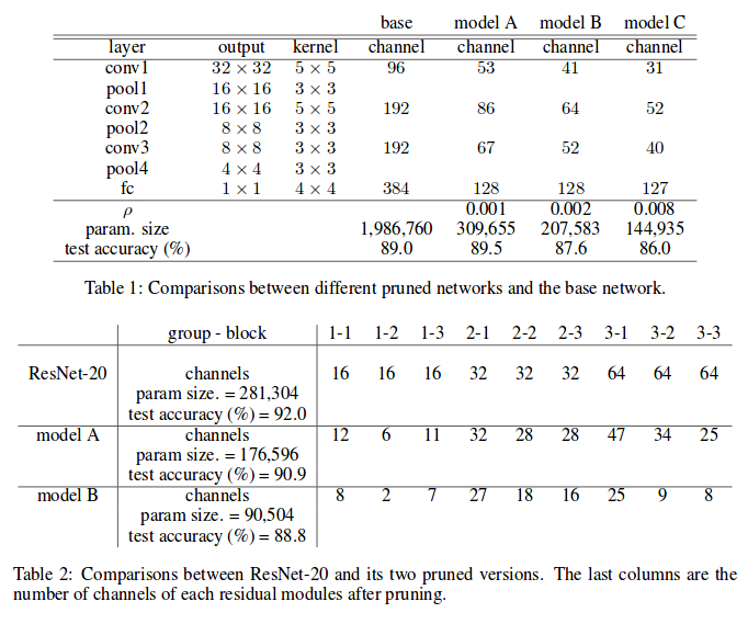
Model A is trained with a sparse penalty of [math]\displaystyle{ \rho = 0.0002 }[/math] for 30 thousand steps, and then increased to [math]\displaystyle{ \rho = 0.001 }[/math]. Model B is trained by taking Model A and increasing the sparse penalty up to 0.002. Similarly Model C is a continuation of Model B with a penalty of 0.008.
For the convNet, reducing the number of parameters in the base model increased the accuracy in model A. This suggests that the base model is over-parameterized. Otherwise, there would be a trade-off of accuracy and model efficiency.
ILSVRC2012 Experiment
The authors note that while ResNet-101 takes hundreds of epochs to train, pruning only takes 5-10, with fine-tuning adding another 2, giving an empirical example how long pruning might take in practice. Both models were trained with an aggressive sparsity penalty of 0.1.
Image Foreground-Background Segmentation Experiment
The authors note that it is common practice to take a network with pre-trained on a large task and fine-tune it to apply it to a different, smaller task. One might expect there might be some extra channels that while useful for the large task, can be omitted for the simpler task. This experiment replicated that use-case by taking a NN originally trained on multiple datasets and applying the proposed pruning method. The authors note that the pruned network actually improves over the original network in all but the most challenging test dataset, which is in line with the initial expectation. The model was trained with a sparsity penalty of 0.5 and the results are shown in table below
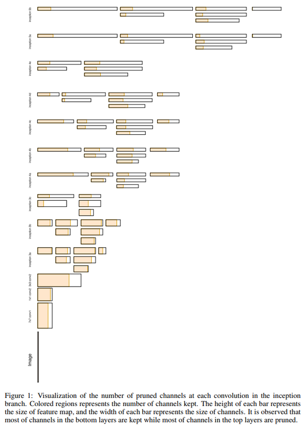
The neural network used in this experiment is composed of two branches:
- An inception branch that locates the foreground objects
- A DenseNet branch to regress the edges
It was found that the pruning primarily affected the inception branch as shown in Figure 1 below. This likely explains the poor performance on more challenging datasets as a result of a higher requirement on foreground objects, which has been impacted by the pruning of the inception branch.
Conclusion
Pruning large neural architectures to fit on low-power devices is an important task. For a real quantitative measure of efficiency, it would be interesting to conduct actual power measurements on the pruned models versus baselines; reduction in FLOPs doesn't necessarily correspond with vastly reduced power since memory accesses dominate energy consumption (Han et al., 2015). However, the reduction in the number of FLOPs and parameters is encouraging, so moderate power savings should be expected.
It would also be interesting to combine multiple approaches, or "throw the whole kitchen sink" at this task. Han et al. (2015) sparked much recent interest by successfully combining weight pruning, quantization, and Huffman coding without loss in accuracy. However, their approach introduced irregular sparsity in the convolutional layers, so a direct comparison cannot be made.
In conclusion, this novel, theoretically-motivated interpretation of channel pruning was successfully applied to several important tasks.
Implementation
A PyTorch implementation is available here: https://github.com/jack-willturner/batchnorm-pruning
References
- Krizhevsky, A., Sutskever, I., & Hinton, G. E. (2012). Imagenet classification with deep convolutional neural networks. In Advances in neural information processing systems (pp. 1097-1105).
- He, K., Zhang, X., Ren, S., & Sun, J. (2016). Deep residual learning for image recognition. In Proceedings of the IEEE conference on computer vision and pattern recognition (pp. 770-778).
- Cheng, Y., Wang, D., Zhou, P., & Zhang, T. (2017). A Survey of Model Compression and Acceleration for Deep Neural Networks. arXiv preprint arXiv:1710.09282.
- Ye, J., Lu, X., Lin, Z., & Wang, J. Z. (2018). Rethinking the Smaller-Norm-Less-Informative Assumption in Channel Pruning of Convolution Layers. arXiv preprint arXiv:1802.00124.
- Li, H., Kadav, A., Durdanovic, I., Samet, H., & Graf, H. P. (2016). Pruning filters for efficient convnets. arXiv preprint arXiv:1608.08710.
- Molchanov, P., Tyree, S., Karras, T., Aila, T., & Kautz, J. (2016). Pruning convolutional neural networks for resource efficient inference.
- Ioffe, S., & Szegedy, C. (2015, June). Batch normalization: Accelerating deep network training by reducing internal covariate shift. In International conference on machine learning (pp. 448-456).
- Gordon, G., & Tibshirani, R. (2012). Subgradient method. https://www.cs.cmu.edu/~ggordon/10725-F12/slides/06-sg-method.pdf
- Beck, A., & Teboulle, M. (2009). A fast iterative shrinkage-thresholding algorithm for linear inverse problems. SIAM journal on imaging sciences, 2(1), 183-202.
- Han, S., Mao, H., & Dally, W. J. (2015). Deep compression: Compressing deep neural networks with pruning, trained quantization and huffman coding. arXiv preprint arXiv:1510.00149


