stat946F18/differentiableplasticity
Differentiable Plasticity \usepackage{amsmath}
Presented by
1. Ganapathi Subramanian, Sriram
Motivation
1. Neural Networks which is the basis of the modern artificial intelligence techniques, is static in nature in terms of architecture. Once a Neural Network is trained the network architecture components (ex. network connections) cannot be changed and thus effectively learning stops with the training step. If a different task needs to be considered, then the agent must be trained again from scratch.
2. Plasticity is the characteristic of biological systems like humans, which is capable of changing the network connections over time. This enables lifelong learning in biological systems and thus is capable of adapting to dynamic changes in the environment with great sample efficiency in the data observed. This is called synaptic plasticity which is based on the Hebb's rule i.e. If a neuron repeatedly takes part in making another neuron fire, the connection between them is strengthened.
3. Differential plasticity is a step in this direction. The plastic connections' behavior is trained using gradient descent so that the previously trained networks can adapt to changing conditions.
Example: Using the current state of the art supervised learning examples, we can train Neural Networks to recognize specific letters that it has seen during training. Using lifelong learning the agent can know about any alphabet, including those that it has never been exposed to during training.
Objectives
The paper has the following objectives:
1. To tackle to problem of meta-learning (learning to learn).
2. To design neural networks with plastic connections with a special emphasis on gradient descent capability for backpropagation training.
3. To use Backpropagation to optimize both the base weights and the amount of plasticity in each connection.
4. To demonstrate the performance of such networks on three complex and different domains namely complex pattern memorization, one shot classification and reinforcement learning.
Related Work
Previous Approaches to solving this problem.
1. Train standard recurrent neural networks to incorporate past experience in their future responses within each episode. For the learning abilities, the RNN is attached with an external content-addressable memory bank. An attention mechanism within the controller network does the read-write to the memory bank and thus enables fast memorization.

2. Augment each weight with a plastic component that automatically grows and decays as a function of inputs and outputs. All connection have the same non-trainable plasticity and only the corresponding weights are trained. Recent approaches have tried fast-weights which augments recurrent networks with fast-changing Hebbian weights and computes activations at each step. The network has a high bias towards the recently seen patterns.

3. Optimize the learning rule itself instead of the connections. A parametrized learning rule is used where the structure of the network is fixed beforehand.

4. Have all the weight updates to be computed on the fly by the network itself or by a separate network at each time step. Pros are the flexibility and the cons are the large learning burden placed on the network.

5. Perform gradient descent via propagation during the episode. The meta-learning involves training the base network for it to be fine-tuned using additional gradient descent.

6. For classification tasks, a separate embedding is trained to discriminate between different classes. Classification is then a comparison between the embedding of the test and example instances.
The superiority of the trainable synaptic plasticity for the meta-learning approach in the paper:
1. Great potential for flexibility. Example, Memory Networks enforce a specific memory storage model in which memories must be embedded in fixed-size vectors and retrieved through some attentional mechanism. In contrast, trainable synaptic plasticity translates into very different forms of memory, the exact implementation of which can be determined by (trainable) network structure.
2. Fixed-weight recurrent networks, meanwhile, require neurons to be used for both storage and computation which increases the computational burdens on neurons. This is avoided in the approach suggested in the paper.
3. Non-trainable plasticity networks can exploit network connectivity for storage of short-term information, but their uniform, non-trainable plasticity imposes a stereotypical behavior on these memories. In the synaptic plasticity, the amount and rate of plasticity are actively molded by the mechanism itself. Also, it allows for more sustained memory.
Model
The formulation proposed in the paper is in such a way that the plastic and non-plastic components for each connection are kept separate, while multiple Hebbian rules can be easily defined.
Model Components:
1. A connection between any two neurons [math]\displaystyle{ i }[/math] and [math]\displaystyle{ j }[/math] has both a fixed component and a plastic component.
2. The fixed part is just a traditional connection weight [math]\displaystyle{ w_{i,j} }[/math] . The plastic part is stored in a Hebbian trace [math]\displaystyle{ H_{i,j} }[/math], which varies during a lifetime according to ongoing inputs and outputs.
3. The relative importance of plastic and fixed components in the connection is structurally determined by the plasticity coefficient [math]\displaystyle{ \alpha_{i,j} }[/math], which multiplies the Hebbian trace to form the full plastic component of the connection.
The network equations are as follows:
[math]\displaystyle{
x_j(t) = \sigma{\displaystyle \sum_{i \in \text{inputs}}[(w_{i,j}x_i(t-1) + \alpha_{i,j} H_{i,j}(t))x_i(t-1)] }
}[/math]
[math]\displaystyle{ H_{i,j}(t+1) = \eta x-i(t-1) x_j(t) + (1 - \eta) H_{i,j}(t) }[/math]
The [math]\displaystyle{ x_j(t) }[/math] is the output of neuron [math]\displaystyle{ j }[/math]. Here the first equation gives the activation function, where the [math]\displaystyle{ w_{i,j} }[/math] is a fixed component and the remaining term ([math]\displaystyle{ \alpha_{i,j} H_{i,j}(t))x_i(t-1) }[/math]) is a plastic component. The [math]\displaystyle{ \sigma }[/math] is a nonlinear function. It is always chosed to be tanh in this paper. The [math]\displaystyle{ H_{i,j} }[/math] in the second equation is updated as a function of ongoing inputs and outputs.
From first equation above, a connection can be fully fixed if [math]\displaystyle{ \alpha = 0 }[/math] or fully plastic if [math]\displaystyle{ w = 0 }[/math] or have both a fixed and plastic components.
The terms [math]\displaystyle{ w_{i,j} }[/math] and [math]\displaystyle{ \alpha_{i,j} }[/math] are the structural parameters trained by gradient descent. The [math]\displaystyle{ \eta }[/math] which denotes the learning rate is also an optimized parameter of the network. After this training, the agent can learn automatically from ongoing experience. In equation 2 above, the [math]\displaystyle{ \eta }[/math] could make the Hebbian traces to decay to 0 in the absence of input. So another form of the equation is as follows:
[math]\displaystyle{
H_{i,j}(t+1) = H_{i,j}(t) + \eta x_j(t)(x_i(t-1) - x_j(t)H_{i,j}(t)]
}[/math]
Experiment1 - Binary Pattern Memorization
This test involves quickly memorizing sets of arbitrary high-dimensional patterns and reconstructing the same while being exposed to partial, degraded versions of them. This is a very simple test as it is already known that hand designed recurrent networks with a Hebbian plastic connection can already solve it for binary patterns.
Steps in the experiment:
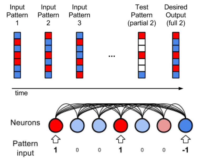
 1) The network is a set of five binary patterns in succession as shown in the above figure. Each of these patterns has 1000 elements each of which has one of the binary value (1 or -1). Here 1 corresponds to dark red and -1 corresponds to dark blue.
2) The few shot learning paradigm is followed, where each pattern is shown for 10-time steps, with 3-time steps of zero input between the presentations and the whole sequence of patterns is presented 3 times in random order.
3) One of the presented patterns is chosen in random order and degraded by setting half of its bits to 0.
4) This degraded pattern is then fed to the network. The network has to reproduce the correct full pattern in its output using its memory that it developed during training.
The architecture of the network is described as follows:
1) It is a fully connected RNN with one neuron per pattern element, plus one fixed-output neuron. There is a total of 1001 neurons.
2) Value of each neuron is clamped to the value of the corresponding element in the pattern if the value is not 0. If the value is 0, the corresponding neurons do not receive pattern input and must use what it gets from lateral connections and reconstruct the correct, expected output values.
3) Outputs are read from the activation of the neurons.
4) The performance evaluation is done by computing the loss between the final network output and the correct expected pattern.
5) The gradient of the error over the $w_{i,j}$ and the $\alpha_{i,j}$ coefficients is computed by backpropagation and optimized through Adam solver with learning rate 0.001.
6) The simple decaying Hebbian formula in Equation 2 is used to update the Hebbian traces. Each network has 2 trainable parameters $w$ and $\alpha$ for each connection, thus there are a total $1001 \times 1001 \times 2 = 2004002$ trainable parameters.
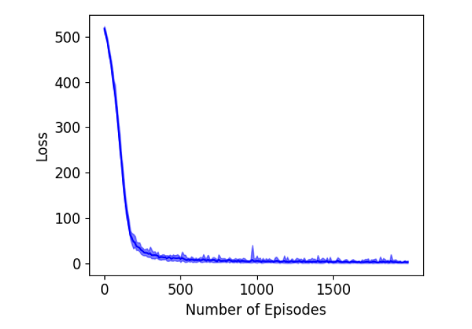
The results are shown in the above figure where 10 runs are considered. The error becomes quite low after about 200 episodes of training.
Comparison with Non-Plastic Networks:
1) Nonplastic networks can solve this task but require additional neurons to solve this task in principle. In practice, the authors say that the task is not solved using Non-plastic RNN or LSTM.
2) The results figure above also shows the results using non-plastic networks. The best results required the addition of 2000 extra neurons.
3) For non-plastic RNN, the error flattens around 0.13 which is quite high. Using LSTMs, the task can be solved albeit imperfectly and also the error rate reduces drastically t0 around 0.001.
4) The plastic network solves the task very quickly with the mean error going below 0.01 within 2000 episodes which are mentioned to be 250 times faster than the LSTM.
