stat946F18/Autoregressive Convolutional Neural Networks for Asynchronous Time Series
This page is a summary of the paper "Autoregressive Convolutional Neural Networks for Asynchronous Time Series" by Mikołaj Binkowski, Gautier Marti, Philippe Donnat. It was published at ICML in 2018. The code for this paper is provided here.
Introduction
In this paper, the authors propose a deep convolutional network architecture called Significance-Offset Convolutional Neural Network for regression of multivariate asynchronous time series. The model is inspired by standard autoregressive (AR) models and gating systems used in recurrent neural networks. The model is evaluated on various time series data including:
- Hedge fund proprietary dataset of over 2 million quotes for a credit derivative index,
- An artificially generated noisy auto-regressive series,
- A UCI household electricity consumption dataset.
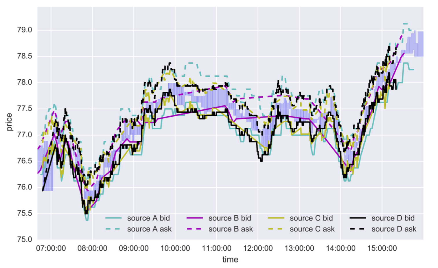
This paper focused on time series that have multivariate and noisy signals, especially financial data. Financial time series is challenging to predict due to their low signal-to-noise ratio and heavy-tailed distributions. For example, the same signal (e.g. price of a stock) is obtained from different sources (e.g. financial news, an investment bank, financial analyst etc.) asynchronously. Each source may have a different bias or noise. (Figure 1) The investment bank with more clients can update their information more precisely than the investment bank with fewer clients, which means the significance of each past observations may depend on other factors that change in time. Therefore, the traditional econometric models such as AR, VAR (Vector Autoregressive Model), VARMA (Vector Autoregressive Moving Average Model) [1] might not be sufficient. However, their relatively good performance could allow us to combine such linear econometric models with deep neural networks that can learn highly nonlinear relationships. This model is inspired by the gating mechanism which is successful in RNNs and Highway Networks.
Time series forecasting is focused on modeling the predictors of future values of time series given their past. As in many cases the relationship between past and future observations is not deterministic, this amounts to expressing the conditional probability distribution as a function of the past observations: The time series forecasting problem can be expressed as a conditional probability distribution below,
This forecasting problem has been approached almost independently by econometrics and machine learning communities. In this paper, the authors focus on modeling the predictors of future values of time series given their past values.
The reasons that financial time series are particularly challenging:
- Low signal-to-noise ratio and heavy-tailed distributions.
- Being observed different sources (e.g. financial news, analysts, portfolio managers in hedge funds, market-makers in investment banks) in asynchronous moments of time. Each of these sources may have a different bias and noise with respect to the original signal that needs to be recovered.
- Data sources are usually strongly correlated and lead-lag relationships are possible (e.g. a market-maker with more clients can update its view more frequently and precisely than one with fewer clients).
- The significance of each of the available past observations might be dependent on some other factors that can change in time. Hence, the traditional econometric models such as AR, VAR, VARMA might not be sufficient.
The predictability of financial dataset still remains an open problem and is discussed in various publications [2].

The paper also provides empirical evidence that their model which combines linear models with deep learning models could perform better than just DL models like CNN, LSTMs and Phased LSTMs.
Related Work
Time series forecasting
From recent proceedings in main machine learning venues i.e. ICML, NIPS, AISTATS, UAI, we can notice that time series are often forecasted using Gaussian processes[3,4], especially for irregularly sampled time series[5]. Though still largely independent, combined models have started to appear, for example, the Gaussian Copula Process Volatility model[6]. For this paper, the authors use coupling AR models and neural networks to achieve such combined models.
Although deep neural networks have been applied into many fields and produced satisfactory results, there still is little literature on deep learning for time series forecasting. More recently, the papers include Sirignano (2016)[7] that used 4-layer perceptrons in modeling price change distributions in Limit Order Books and Borovykh et al. (2017)[8] who applied more recent WaveNet architecture to several short univariate and bivariate time-series (including financial ones). Heaton et al. (2016)[9] claimed to use autoencoders with a single hidden layer to compress multivariate financial data. Neil et al. (2016)[10] presented augmentation of LSTM architecture suitable for asynchronous series, which stimulates learning dependencies of different frequencies through the time gate. The LSTM architecture has three "gates", the input gate, the forget gate, and the update gate. It performs well in practice because it allows the RNN architecture to be able to take into account events happened a long time ago. Traditionally, RNN architectures are heavily influenced by recent events, but LSTM overcomes that by updating the weights in the three newly introduced gates.
In this paper, the authors examine the capabilities of several architectures (CNN, residual network, multi-layer LSTM, and phase LSTM) on AR-like artificial asynchronous and noisy time series, household electricity consumption dataset, and on real financial data from the credit default swap market with some inefficiencies.
AR Model
An autoregressive (AR) model describes the next value in a time-series as a combination of previous values, scaling factors, a bias, and noise (source). It is a representation of a type of random process and is used to describe certain time varying processes. The AR model specifies that the output variable depends lienarly on tis own previous values and on a stochastic term which is imperfectly predictable. Tus the model is in the form of a stochastic difference equation. For a p-th order (relating the current state to the p last states), the equation of the model is:
[math]\displaystyle{ X_t = c + \sum_{i=1}^p \varphi_i X_{t-i}+ \varepsilon_t \, }[/math] (equation source)
With parameters/coefficients [math]\displaystyle{ \varphi_i }[/math], constant [math]\displaystyle{ c }[/math], and noise [math]\displaystyle{ \varepsilon_t }[/math] This can be extended to vector form to create the VAR model mentioned in the paper.
Gating and weighting mechanisms
Gating mechanism for neural networks has ability to overcome the problem of vanishing gradients, and can be expressed as [math]\displaystyle{ f(x)=c(x) \otimes \sigma(x) }[/math], where [math]\displaystyle{ f }[/math] is the output function, [math]\displaystyle{ c }[/math] is a "candidate output" (a nonlinear function of [math]\displaystyle{ x }[/math]), [math]\displaystyle{ \otimes }[/math] is an element-wise matrix product, and [math]\displaystyle{ \sigma : \mathbb{R} \rightarrow [0,1] }[/math] is a sigmoid non-linearity that controls the amount of output passed to the next layer. Different composition of functions of the same type as described above have proven to be an essential ingredient in popular recurrent architecture such as LSTM and GRU[11].
The main purpose of the proposed gating system is to weight the outputs of the intermediate layers within neural networks, and is most closely related to softmax gating used in MuFuRu(Multi-Function Recurrent Unit)[12], i.e. [math]\displaystyle{ f(x) = \sum_{l=1}^L p^l(x) \otimes f^l(x)\text{,}\ p(x)=\text{softmax}(\widehat{p}(x)), }[/math], where [math]\displaystyle{ (f^l)_{l=1}^L }[/math]are candidate outputs (composition operators in MuFuRu), [math]\displaystyle{ (\widehat{p}^l)_{l=1}^L }[/math]are linear functions of inputs.
This idea is also successfully used in attention networks[13] such as image captioning and machine translation. In this paper, the proposed method is similar as, the separate inputs (time series steps in this case) are weighted in accordance with learned functions of these inputs. The difference is that the functions are modelled using multi-layer CNNs. Another difference is that the proposed method is not using recurrent layers, which enables the network to remember parts of the sentence/image already translated/described.
Motivation
There are mainly five motivations that are stated in the paper by the authors:
- The forecasting problem in this paper has been done almost independently by econometrics and machine learning communities. Unlike in machine learning, research in econometrics is more likely to explain variables rather than improving out-of-sample prediction power. These models tend to 'over-fit' on financial time series, their parameters are unstable and have poor performance on out-of-sample prediction.
- It is difficult for the learning algorithms to deal with time series data where the observations have been made irregularly. Although Gaussian processes provide a useful theoretical framework that is able to handle asynchronous data, they are not suitable for financial datasets, which often follow heavy-tailed distribution .
- Predictions of autoregressive time series may involve highly nonlinear functions if sampled irregularly. For AR time series with higher order and have more past observations, the expectation of it [math]\displaystyle{ \mathbb{E}[X(t)|{X(t-m), m=1,...,M}] }[/math] may involve more complicated functions that in general may not allow closed-form expression.
- In practice, the dimensions of multivariate time series are often observed separately and asynchronously, such series at fixed frequency may lead to lose information or enlarge the dataset, which is shown in Figure 2(a). Therefore, the core of the proposed architecture SOCNN represents separate dimensions as a single one with dimension and duration indicators as additional features(Figure 2(b)).
- Given a series of pairs of consecutive input values and corresponding durations, [math]\displaystyle{ x_n = (X(t_n),t_n-t_{n-1}) }[/math]. One may expect that LSTM may memorize the input values in each step and weight them at the output according to the duration, but this approach may lead to an imbalance between the needs for memory and for linearity. The weights that are assigned to the memorized observations potentially require several layers of nonlinearity to be computed properly, while past observations might just need to be memorized as they are.

Model Architecture
Suppose there exists a multivariate time series [math]\displaystyle{ (x_n)_{n=0}^{\infty} \subset \mathbb{R}^d }[/math], we want to predict the conditional future values of a subset of elements of [math]\displaystyle{ x_n }[/math]
where [math]\displaystyle{ I=\{i_1,i_2,...i_{d_I}\} \subset \{1,2,...,d\} }[/math] is a subset of features of [math]\displaystyle{ x_n }[/math].
Let [math]\displaystyle{ \textbf{x}_n^{-M} = (x_{n-m})_{m=1}^M }[/math].
The estimator of [math]\displaystyle{ y_n }[/math] can be expressed as:
The estimate is the summation of the columns of the matrix in bracket. Here
- [math]\displaystyle{ F,S : \mathbb{R}^{d \times M} \rightarrow \mathbb{R}^{d_I \times M} }[/math] are neural networks.
- [math]\displaystyle{ S }[/math] is a fully convolutional network which is composed of convolutional layers only.
- [math]\displaystyle{ F(\textbf{x}_n^{-M}) = W \otimes [\text{off}(x_{n-m}) + x_{n-m}^I)]_{m=1}^M }[/math]
- [math]\displaystyle{ W \in \mathbb{R}^{d_I \times M} }[/math]
- [math]\displaystyle{ \text{off}: \mathbb{R}^d \rightarrow \mathbb{R}^{d_I} }[/math] is a multilayer perceptron.
- [math]\displaystyle{ \sigma }[/math] is a normalized activation function independent at each row, i.e. [math]\displaystyle{ \sigma ((a_1^T, ..., a_{d_I}^T)^T)=(\sigma(a_1)^T,..., \sigma(a_{d_I})^T)^T }[/math]
- for any [math]\displaystyle{ a_{i} \in \mathbb{R}^{M} }[/math]
- and [math]\displaystyle{ \sigma }[/math] is defined such that [math]\displaystyle{ \sigma(a)^{T} \mathbf{1}_{M}=1 }[/math] for any [math]\displaystyle{ a \in \mathbb{R}^M }[/math].
- [math]\displaystyle{ \otimes }[/math] is element-wise matrix multiplication (also known as Hadamard matrix multiplication).
- [math]\displaystyle{ A.,_m }[/math] denotes the m-th column of a matrix A.
Since [math]\displaystyle{ \sum_{m=1}^M W.,_m=W\cdot(1,1,...,1)^T }[/math] and [math]\displaystyle{ \sum_{m=1}^M S.,_m=S\cdot(1,1,...,1)^T }[/math], we can express [math]\displaystyle{ \hat{y}_n }[/math] as:
This is the proposed network, Significance-Offset Convolutional Neural Network, [math]\displaystyle{ \text{off} }[/math] and [math]\displaystyle{ S }[/math] in the equation are corresponding to Offset and Significance in the name respectively. Figure 3 shows the scheme of network.

The form of [math]\displaystyle{ \tilde{y}_n }[/math] ensures the separation of the temporal dependence (obtained in weights [math]\displaystyle{ W_m }[/math]). [math]\displaystyle{ S }[/math], which represents the local significance of observations, is determined by its filters which capture local dependencies and are independent of the relative position in time, and the predictors [math]\displaystyle{ \text{off}(x_{n-m}) }[/math] are completely independent of position in time. An adjusted single regressor for the target variable is provided by each past observation through the offset network. Since in asynchronous sampling procedure, consecutive values of x come from different signals and might be heterogeneous, therefore adjustment of offset network is important. In addition, significance network provides data-dependent weight for each regressor and sums them up in an autoregressive manner.
Relation to asynchronous data
One common problem of time series is that durations are varying between consecutive observations, the paper states two ways to solve this problem
- Data preprocessing: aligning the observations at some fixed frequency e.g. duplicating and interpolating observations as shown in Figure 2(a). However, as mentioned in the figure, this approach will tend to loss of information and enlarge the size of the dataset and model complexity.
- Add additional features: Treating the duration or time of the observations as additional features, it is the core of SOCNN, which is shown in Figure 2(b).
Loss function
The L2 error is a natural loss function for the estimators of expected value: [math]\displaystyle{ L^2(y,y')=||y-y'||^2 }[/math]
The output of the offset network is series of separate predictors of changes between corresponding observations [math]\displaystyle{ x_{n-m}^I }[/math] and the target value[math]\displaystyle{ y_n }[/math], this is the reason why we use auxiliary loss function, which equals to mean squared error of such intermediate predictions:
The total loss for the sample [math]\displaystyle{ \textbf{x}_n^{-M},y_n) }[/math] is then given by:
where [math]\displaystyle{ \widehat{y}_n }[/math] was mentioned before, [math]\displaystyle{ \alpha \geq 0 }[/math] is a constant.
Experiments
The paper evaluated SOCNN architecture on three datasets: artificially generated datasets, household electric power consumption dataset, and the financial dataset of bid/ask quotes provided by several market participants active in the credit derivatives market. Comparing its performance with simple CNN, single and multiplayer LSTM, Phased LSTM and 25-layer ResNet. Apart from the evaluation of the SOCNN architecture, the paper also discussed the impact of network components such as auxiliary loss and the depth of the offset sub-network. The code and datasets are available here.
Datasets
Artificial data: They generated 4 artificial series, [math]\displaystyle{ X_{K \times N} }[/math], where [math]\displaystyle{ K \in \{16,64\} }[/math]. Therefore there is a synchronous and an asynchronous series for each K value. Note that a series with K sources is K + 1-dimensional in synchronous case and K + 2-dimensional in asynchronous case. The base series in all processes was a stationary AR(10) series. Although that series has the true order of 10, in the experimental setting the input data included past 60 observations. The rationale behind that is twofold: not only is the data observed in irregular random times but also in real–life problems the order of the model is unknown.
Electricity data: This UCI dataset contains 7 different features excluding date and time. The features include global active power, global reactive power, voltage, global intensity, sub-metering 1, sub-metering 2 and sub-metering 3, recorded every minute for 47 months. The data has been altered so that one observation contains only one value of 7 features, while durations between consecutive observations are ranged from 1 to 7 minutes. The goal is to predict all 7 features for the next time step.
Non-anonymous quotes: The dataset contains 2.1 million quotes from 28 different sources from different market participants such as analysts, banks etc. Each quote is characterized by 31 features: the offered price, 28 indicators of the quoting source, the direction indicator (the quote refers to either a buy or a sell offer) and duration from the previous quote. For each source and direction, we want to predict the next quoted price from this given source and direction considering the last 60 quotes.

Training details
They applied grid search on some hyperparameters in order to get the significance of its components. The hyperparameters include the offset sub-network's depth and the auxiliary weight [math]\displaystyle{ \alpha }[/math]. For offset sub-network's depth, they use 1, 10,1 for artificial, electricity and quotes dataset respectively; and they compared the values of [math]\displaystyle{ \alpha }[/math] in {0,0.1,0.01}.
They chose LeakyReLU as activation function for all networks:
They use the same number of layers, same stride and similar kernel size structure in CNN. In each trained CNN, they applied max pooling with the pool size of 2 every 2 convolutional layers.
Table 1 presents the configuration of network hyperparameters used in comparison

Network Training
The training and validation data were sampled randomly from the first 80% of timesteps in each series, with a ratio of 3 to 1. The remaining 20% of the data was used as a test set.
All models were trained using Adam optimizer because the authors found that its rate of convergence was much faster than standard Stochastic Gradient Descent in early tests.
They used a batch size of 128 for artificial and electricity data, and 256 for quotes dataset, and applied batch normalization between each convolution and the following activation.
At the beginning of each epoch, the training samples were randomly sampled. To prevent overfitting, they applied dropout and early stopping.
Weights were initialized using the normalized uniform procedure proposed by Glorot & Bengio (2010).[14]
The authors carried out the experiments on Tensorflow and Keras and used different GPU to optimize the model for different datasets. The artificial and electricity data was optimized using one NVIDIA K20, while the quotes data used only an Intel Core i7-6700 CPU.
Results
Table 2 shows all results performed from all datasets.

We can see that SOCNN outperforms in all asynchronous artificial, electricity and quotes datasets. For synchronous data, LSTM might be slightly better, but SOCNN almost has the same results with LSTM. Phased LSTM and ResNet have performed really bad on an artificial asynchronous dataset and quotes dataset respectively. Notice that having more than one layer of offset network would have a negative impact on results. Also, the higher weights of auxiliary loss([math]\displaystyle{ \alpha }[/math]considerably improved the test error on an asynchronous dataset, see Table 3. However, for other datasets, its impact was negligible. This makes it hard to justify the introduction of the auxiliary loss function [math]\displaystyle{ L^{aux} }[/math].
Also, using artificial dataset as the experimental result is not a good practice in this paper. This is essentially an application paper, and such dataset makes results hard to reproduce, and cannot support the performance claim of the model.

In general, SOCNN has a significantly lower variance of the test and validation errors, especially in the early stage of the training process and for quotes dataset. This effect can be seen in the learning curves for Asynchronous 64 artificial dataset presented in Figure 5.

Finally, we want to test the robustness of the proposed model SOCNN, adding noise terms to asynchronous 16 datasets and check how these networks perform. The result is shown in Figure 6.

From Figure 6, the purple lines and green lines seem to stay at the same position in the training and testing process. SOCNN and single-layer LSTM are most robust and least prone to overfitting comparing to other networks.
Conclusion and Discussion
In this paper, the authors have proposed a new architecture called Significance-Offset Convolutional Neural Network, which combines AR-like weighting mechanism and convolutional neural network. This new architecture is designed for high-noise asynchronous time series and achieves outperformance in forecasting several asynchronous time series compared to popular convolutional and recurrent networks.
The SOCNN can be extended further by adding intermediate weighting layers of the same type in the network structure. Another possible extension but needs further empirical studies is that we consider not just [math]\displaystyle{ 1 \times 1 }[/math] convolutional kernels on the offset sub-network. Also, this new architecture might be tested on other real-life datasets with relevant characteristics in the future, especially on econometric datasets and more generally for time series (stochastic processes) regression.
Critiques
- The paper is most likely an application paper, and the proposed new architecture shows improved performance over baselines in the asynchronous time series.
- The quote data cannot be reached as they are proprietary. Also, only two datasets available.
- The 'Significance' network was described as critical to the model in paper, but they did not show how the performance of SOCNN with respect to the significance network.
- The transform of the original data to asynchronous data is not clear.
- The experiments on the main application are not reproducible because the data is proprietary.
- The way that train and test data were split is unclear. This could be important in the case of the financial data set.
- Although the auxiliary loss function was mentioned as an important part, the advantages of it was not too clear in the paper. Maybe it is better that the paper describes a little more about its effectiveness. It helped achieve more stable test error throughout training in many cases.
- It was not mentioned clearly in the paper whether the model training was done on a rolling basis for time series forecasting.
- The noise term used in section 5's model robustness analysis uses evenly distributed noise (see Appendix B). While the analysis is a good start, analysis with different noise distributions would make the findings more generalizable.
- The paper uses financial/economic data as one of its testing data set. Instead of comparing neural network models such as CNN which is known to work badly on time series data, it would be much better if the author compared to well-known econometric time series models such as GARCH and VAR.
- The paper does not specify how training and testing set are separated in detail, which is quite important in time-series problems. Moreover, rolling or online-based learning scheme should be used in comparison, since they are standard in time-series prediction tasks.
References
[1] Hamilton, J. D. Time series analysis, volume 2. Princeton university press Princeton, 1994.
[2] Fama, E. F. Efficient capital markets: A review of theory and empirical work. The journal of Finance, 25(2):383–417, 1970.
[3] Petelin, D., Sˇindela ́ˇr, J., Pˇrikryl, J., and Kocijan, J. Financial modeling using gaussian process models. In Intelligent Data Acquisition and Advanced Computing Systems (IDAACS), 2011 IEEE 6th International Conference on, volume 2, pp. 672–677. IEEE, 2011.
[4] Tobar, F., Bui, T. D., and Turner, R. E. Learning stationary time series using Gaussian processes with nonparametric kernels. In Advances in Neural Information Processing Systems, pp. 3501–3509, 2015.
[5] Hwang, Y., Tong, A., and Choi, J. Automatic construction of nonparametric relational regression models for multiple time series. In Proceedings of the 33rd International Conference on Machine Learning, 2016.
[6] Wilson, A. and Ghahramani, Z. Copula processes. In Advances in Neural Information Processing Systems, pp. 2460–2468, 2010.
[7] Sirignano, J. Extended abstract: Neural networks for limit order books, February 2016.
[8] Borovykh, A., Bohte, S., and Oosterlee, C. W. Conditional time series forecasting with convolutional neural networks, March 2017.
[9] Heaton, J. B., Polson, N. G., and Witte, J. H. Deep learning in finance, February 2016.
[10] Neil, D., Pfeiffer, M., and Liu, S.-C. Phased lstm: Accelerating recurrent network training for long or event-based sequences. In Advances In Neural Information Process- ing Systems, pp. 3882–3890, 2016.
[11] Chung, J., Gulcehre, C., Cho, K., and Bengio, Y. Empirical evaluation of gated recurrent neural networks on sequence modeling, December 2014.
[12] Weissenborn, D. and Rockta ̈schel, T. MuFuRU: The Multi-Function recurrent unit, June 2016.
[13] Cho, K., Courville, A., and Bengio, Y. Describing multi- media content using attention-based Encoder–Decoder networks. IEEE Transactions on Multimedia, 17(11): 1875–1886, July 2015. ISSN 1520-9210.
[14] Glorot, X. and Bengio, Y. Understanding the difficulty of training deep feedforward neural net- works. In In Proceedings of the International Con- ference on Artificial Intelligence and Statistics (AIS- TATSaˆ10). Society for Artificial Intelligence and Statistics, 2010.