stat841f14: Difference between revisions
RaniaIbrahim (talk | contribs) |
RaniaIbrahim (talk | contribs) (→Proof) |
||
| Line 770: | Line 770: | ||
<math> \sum_{i,j} w_{ij} * (f_i - f_j)^2 </math> | <math> \sum_{i,j} w_{ij} * (f_i - f_j)^2 </math> | ||
< | <br> | ||
we have 4 cases (<math> i \in A </math> & <math> j \in A </math>, <math> i \in A </math> & <math> j \in \bar{A} </math>, <math> i \in \bar{A} </math> & <math> j \in {A} </math>, <math> i \in \bar{A} </math> & <math> j \in \bar{A} </math>) | we have 4 cases (<math> i \in A </math> & <math> j \in A </math>, <math> i \in A </math> & <math> j \in \bar{A} </math>, <math> i \in \bar{A} </math> & <math> j \in {A} </math>, <math> i \in \bar{A} </math> & <math> j \in \bar{A} </math>) | ||
Revision as of 00:44, 10 October 2014
Editor Sign Up
Principal components analysis (Lecture 1: Sept. 10, 2014)
Introduction
Principal Component Analysis (PCA), first invented by Karl Pearson in 1901, is a statistical technique for data analysis. Its main purpose is to reduce the dimensionality of the data.
Suppose there is a set of data points in a d-dimensional space. The goal of PCA is to find a linear subspace with lower dimensionality p (p [math]\displaystyle{ \leq }[/math] d), such that maximum variance is retained in this lower-dimensional space. The linear subspace can be specified by d orthogonal vectors, such as [math]\displaystyle{ u_1 , u_2 , ... , u_d }[/math] which form a new coordinate system, called 'principle components'. In other words, PCA aims to reduce the dimensionality of the data, while preserving its information (or minimizing the loss of information). Information comes from variation. In other words, the more variation captured in the lower dimension, the more information preserved. For example, if all data points have the same value along one dimension, then that dimension does not carry any information. So, to preserve information, the subspace need to contain components (or dimensions) along which, data has most of its variability. However, finding a linear subspace with lower dimensionality which include all data points is not possible in practical problems and loss of information is inevitable. Through PCA, we try to reduce this loss and capture most of the features of data.
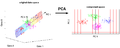
Figure below, demonstrates an example of PCA. Data is transformed from original 3D space to 2D coordinate system where each coordinate is a principal component.
-
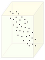
Data in original Space
-
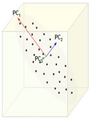
Extraction of the principal components
-
Reduction of dimensionality by keeping the first two principal components and removing the third one


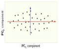
Now, consider the ability of two of the above examples' components (PC1 and PC2) to retain information from the original data. The data in the original space is projected onto each of these two components separately in the below figure. Notice that PC1 is better able to capture the variation in the original data than PC2 alone. If reducing the original d=3 dimensional data to p=1 dimension, PC1 is therefore preferable to PC2.

PCA Plot example
For example<ref> https://onlinecourses.science.psu.edu/stat857/sites/onlinecourses.science.psu.edu.stat857/files/lesson05/PCA_plot.gif </ref>, in the top left corner of the image below, the point [math]\displaystyle{ x_1 }[/math] showed in two-dimensional and it's coordinates are [math]\displaystyle{ (x_i, 1) }[/math] and [math]\displaystyle{ (x_i, 2) }[/math]
All the red points in the plot represented by their projected values on the two original coordinators (Feature 1, Feature 2).
In PCA technique, it uses new coordinators (showed in green). As coordinate system changed, the points also are shown by their new pair of coordinate values for example [math]\displaystyle{ (z_i, 1) }[/math] and [math]\displaystyle{ (z_i, 2) }[/math]. These values are determined by original vector, and the relation between the rotated coordinates and the original ones.

In the original coordinates the two vectors [math]\displaystyle{ x_1 }[/math] and [math]\displaystyle{ x_2 }[/math] are not linearly uncorrelated. In other words, after applying PCA, if there are two principal component, and use those as the new coordinates, then it is guaranteed that the data along the two coordinates have correlation = 0
By rotating the coordinates we performed an orthonormal transform on the data. After the transform, the correlation is removed - which is the whole point of PCA.
As an example of an extreme case where all of the points lie on a straight line, which in the original coordinates system it is needed two coordinates to describe these points.
In short, after rotating the coordinates, we need only one coordinate and clearly the value on the other one is always zero. This example shows PCA's dimension reduction in an extreme case while in real world points may not fit exactly on a line, but only approximately.
PCA applications
As mentioned, PCA is a method to reduce data dimension if possible to principal components such that those PCs cover as much data variation as possible. This technique is useful in different type of applications which involve data with a huge dimension like data pre-processing, neuroscience, computer graphics, meteorology, oceanography, gene expression, economics, and finance among of all other applications.
Data usually is represented by lots of variables. In data preprocessing, PCA is a technique to select a subset of variables in order to figure our best model for data. In neuroscience, PCA used to identify the specific properties of a stimulus that increase a neuron’s probability of generating an action potential.
Figures below show some example of PCA in real world applications. Click to enlarge.
-
Finding two principal components of original data in 2D space. Components of data are highly correlated in original space. So they can be substituted by just one principal component, PC1, which has more than %99 of total variance of data.
-
PCA in Neuroscience. Data in different classes in 3 dimensional space is mapped to a 2 dimensional space using PCA. The mapped data is clearly linearly sparable.

Mathematical details
PCA is a transformation from original space to a linear subspace with a new coordinate system. Each coordinate of this subspace is called a Principle Component. First principal component is the coordinate of this system along which the data points has the maximum variation. That is, if we project the data points along this coordinate, maximum variance of data is obtained (compared to any other vector in original space). Second principal component is the coordinate in the direction of the second greatest variance of the data, and so on.
Lets denote the basis of original space by [math]\displaystyle{ \mathbf{v_1} }[/math], [math]\displaystyle{ \mathbf{v_2} }[/math], ... , [math]\displaystyle{ \mathbf{v_d} }[/math]. Our goal is to find the principal components (coordinate of the linear subspace), denoted by [math]\displaystyle{ \mathbf{u_1} }[/math], [math]\displaystyle{ \mathbf{u_2} }[/math], ... , [math]\displaystyle{ \mathbf{u_p} }[/math] in the hope that [math]\displaystyle{ p \leq d }[/math]. First, we would like to obtain the first principal component [math]\displaystyle{ \mathbf{u_1} }[/math] or the components in the direction of maximum variance. This component can be treated as a vector in the original space and so is written as a linear combination of the basis in original space.
[math]\displaystyle{ \mathbf{u_1}=w_1\mathbf{v_1}+w_2\mathbf{v_2}+...+w_d\mathbf{v_d} }[/math]
Vector [math]\displaystyle{ \mathbf{w} }[/math] contains the weight of each basis in this combination.
[math]\displaystyle{ \mathbf{w}=\begin{bmatrix} w_1\\w_2\\w_3\\...\\w_d \end{bmatrix} }[/math]
Suppose we have n data points in the original space. We represent each data points by [math]\displaystyle{ \mathbf{x_1} }[/math], [math]\displaystyle{ \mathbf{x_2} }[/math], ..., [math]\displaystyle{ \mathbf{x_n} }[/math]. Projection of each point [math]\displaystyle{ \mathbf{x_i} }[/math] on the [math]\displaystyle{ \mathbf{u_1} }[/math] is [math]\displaystyle{ \mathbf{w}^T\mathbf{x_i} }[/math].
Let [math]\displaystyle{ \mathbf{S} }[/math] be the sample covariance matrix of data points in original space. The variance of the projected data points, denoted by [math]\displaystyle{ \Phi }[/math] is
[math]\displaystyle{ \Phi = Var(\mathbf{w}^T \mathbf{x_i}) = \mathbf{w}^T \mathbf{S} \mathbf{w} }[/math]
we would like to maximize [math]\displaystyle{ \Phi }[/math] over set of all vectors [math]\displaystyle{ \mathbf{w} }[/math] in original space. But, this problem is not yet well-defined, because for any choice of [math]\displaystyle{ \mathbf{w} }[/math], we can increase [math]\displaystyle{ \Phi }[/math] by simply multiplying [math]\displaystyle{ \mathbf{w} }[/math] in a positive scalar greater than one. So, we add the following constraint to the problem to bound the length of vector [math]\displaystyle{ \mathbf{w} }[/math]:
[math]\displaystyle{ max \Phi = \mathbf{w}^T \mathbf{S} \mathbf{w} }[/math]
subject to : [math]\displaystyle{ \mathbf{w}^T \mathbf{w} =1 }[/math]
Using Lagrange Multiplier technique we have:
[math]\displaystyle{ L(\mathbf{w} , \lambda ) = \mathbf{w}^T \mathbf{S} \mathbf{w} - \lambda (\mathbf{w}^T \mathbf{w} - 1 ) }[/math]
By taking derivative of [math]\displaystyle{ L }[/math] w.r.t. primary variable [math]\displaystyle{ \mathbf{w} }[/math] we have:
[math]\displaystyle{ \frac{\partial L}{\partial \mathbf{w}}=( \mathbf{S}^T + \mathbf{S})\mathbf{w} -2\lambda\mathbf{w}= 2\mathbf{S}\mathbf{w} -2\lambda\mathbf{w}= 0 }[/math]
Note that [math]\displaystyle{ \mathbf{S} }[/math] is symmetric so [math]\displaystyle{ \mathbf{S}^T = \mathbf{S} }[/math].
From the above equation we have:
[math]\displaystyle{ \mathbf{S} \mathbf{w} = \lambda\mathbf{w} }[/math].
So [math]\displaystyle{ \mathbf{w} }[/math] is the eigenvector and [math]\displaystyle{ \lambda }[/math] is the eigenvalue of the matrix [math]\displaystyle{ \mathbf{S} }[/math] .(Taking derivative of [math]\displaystyle{ L }[/math] w.r.t. [math]\displaystyle{ \lambda }[/math] just regenerate the constraint of the optimization problem.)
By multiplying both sides of the above equation to [math]\displaystyle{ \mathbf{w}^T }[/math] and considering the constraint, we obtain:
[math]\displaystyle{ \Phi = \mathbf{w}^T \mathbf{S} \mathbf{w} = \mathbf{w}^T \lambda \mathbf{w} = \lambda \mathbf{w}^T \mathbf{w} = \lambda }[/math]
The interesting result is that objective function is equal to eigenvalue of the covariance matrix. So, to obtain the first principle component, which maximizes the objective function, we just need the eigenvector corresponding to the largest eigenvalue of [math]\displaystyle{ \mathbf{S} }[/math]. Subsequently, the second principal component is the eigenvector corresponding to the second largest eigenvalue, and so on.
Principal component extraction using singular value decomposition
Singular Value Decomposition (SVD), is a well-known way to decompose any kind of matrix [math]\displaystyle{ \mathbf{A} }[/math] (m by n) into three useful matrices.
[math]\displaystyle{ \mathbf{A} = \mathbf{U}\mathbf{\Sigma}\mathbf{V}^T }[/math].
where [math]\displaystyle{ \mathbf{U} }[/math] is m by m unitary matrix, [math]\displaystyle{ \mathbf{UU^T} = I_m }[/math], each column of [math]\displaystyle{ \mathbf{U} }[/math] is an eigenvector of [math]\displaystyle{ \mathbf{AA^T} }[/math]
[math]\displaystyle{ \mathbf{\Sigma} }[/math] is m by n diagonal matrix, non-zero elements of this matrix are square roots of eigenvalues of [math]\displaystyle{ \mathbf{AA^T} }[/math].
[math]\displaystyle{ \mathbf{V} }[/math] is n by n unitary matrix, [math]\displaystyle{ \mathbf{VV^T} = I_n }[/math], each column of [math]\displaystyle{ \mathbf{V} }[/math] is an eigenvector of [math]\displaystyle{ \mathbf{A^TA} }[/math]
Now, comparing the concepts of PCA and SVD, one may find out that we can perform PCA using SVD.
Let's construct a matrix p by n with our n data points such that each column of this matrix represent one data point in p-dimensional space:
[math]\displaystyle{ \mathbf{X} = [\mathbf{x_1} \mathbf{x_2} .... \mathbf{x_n} ] }[/math]
and make another matrix [math]\displaystyle{ \mathbf{X}^* }[/math] simply by subtracting the mean of data points from [math]\displaystyle{ \mathbf{X} }[/math].
[math]\displaystyle{ \mathbf{X}^* = \mathbf{X} - \mu_X }[/math]
Then we will get a zero-mean version of our data points for which [math]\displaystyle{ \mathbf{X^*} \mathbf{X^{*^T}} }[/math] is the covariance matrix.
So, [math]\displaystyle{ \mathbf{\Sigma} }[/math] and [math]\displaystyle{ \mathbf{U} }[/math] give us the eigenvalues and corresponding eigenvectors of covariance matrix, respectively. We can then easily extract the desired principal components.
MATLAB example
In this example we use different pictures of a man's face with different facial expressions. But, these pictures are noisy. So the face is not easily recognizable. The data set consists of 1965 pictures each 20 by 28. So dimensionality is 20*28= 560.
Our goal is to remove noise using PCA and of course by means of SVD function in matlab. We know that noise is not the main feature that makes these pictures look different, so noise is among least variance components. We first extract the principal components and then remove those which correspond to the least values of eigenvalues of covariance matrix. Here, eigenvalues are sorted in a descending order from column to column of matrix S. For example, the first column of matrix U, which corresponds to the first element in S, is the first principal component.
We then reconstruct the picture using first d principal components. If d is too large, we can not completely remove the noise. If it is too small, we will lose some information from the original data. For example we may lose the facial expression (smile, sadness and etc.). We can change d until we achieve a reasonable balance between noise reduction and information loss.
 >> % loading the noisy data, file "noisy" stores our variable X which contains the pictures
 >> load noisy;
 >>
 >>
 >> % show a sample image in column 1 of matrix X
 >> imagesc(reshape(X(:,1),20,28)')
 >>
 >> % set the color of image to grayscale
 >> colormap gray
 >>
 >> % perform SVD, if X matrix if full rank, will obtain 560 PCs
 >> [U S V] = svd(X);
 >>
 >> d= 10;
 >>
 >> % reconstruct X using only the first d principal components and removing noise
 >> XX = U(:, 1:d)* S(1:d,1:d)*V(:,1:d)' ;
 >>
 >> % show image in column 1 of XX which is a noise reduced version
 >> imagesc(reshape(XX(:,1),20,28)')
PCA continued, Lagrange multipliers, singular value decomposition (SVD) (Lecture 2: Sept. 15, 2014)
Principal component analysis (continued)
PCA is a method to reduce dimensions in data or to extract features from data.
Given a data point in vector form x the goal of PCA is to map x to y where x [math]\displaystyle{ \isin }[/math] [math]\displaystyle{ \real }[/math]d and y [math]\displaystyle{ \isin }[/math] [math]\displaystyle{ \real }[/math]p such that p is much less than d. For example we could map a two-dimensional data point onto any one-dimensional vector in the original 2D space or we could map a three-dimensional data point onto any 2D plane in the original 3D space.
The transformation from [math]\displaystyle{ d }[/math]-dimensional space to [math]\displaystyle{ p }[/math] dimensional space is chosen in such a way that maximum variance is retained in the lower dimensional subspace. This is useful because variance represents the main differences between the data points, which is exactly what we are trying to capture when we perform data visualization. For example, when taking 64-dimensional images of hand-written digits, projecting them onto 2-dimensional space using PCA captures a significant amount of the structure we care about.
-
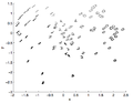
Note that the x-axis captures the value of the number, where 1s are on the left, 2s in the middle and 0s on the right. The y-axis captures tilt.

In terms of data visualization, it is fairly clear why PCA is important. High dimensional data is sometimes impossible to visualize. Even a 3D space can be fairly difficult to visualize, while a 2D space, which can be printed on a piece of paper, is much easier to visualize. If a higher dimensional dataset can be reduced to only 2 dimensions, it can be easily represented by plots and graphs.
In the case of many data points xi in d-dimensional space:
Xdxn = [x1 x2 ... xn]
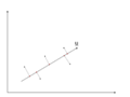
There is an infinite amount of vectors in [math]\displaystyle{ \real }[/math]p to which the points in X can be mapped. When mapping these data points to lower dimensions information will be lost. To preserve as much information as possible the points are mapped to a vector in [math]\displaystyle{ \real }[/math]p which will preserve as much variation in the data as possible. In other words, the data is mapped to the vector in [math]\displaystyle{ \real }[/math]p that will have maximum variance. In the images below, the data points mapped onto u in Mapping 1 have greater variance than in Mapping 2, and thus preserves more information in the data.
-
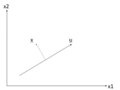
Two dimensional point mapped onto one dimensional vector
-
Mapping 1: Mapping of a two dimensional data set onto a one dimensional vector
-
Mapping 2: Mapping of a two dimensional data set onto a one dimensional vector


The projection of a single data point x on u is uTx (a scalar).
To project n data points onto u compute Y = uTX.
The variance of Y = uTX can be calculated easily as Y is a 1 by n vector.
In higher dimensional space [math]\displaystyle{ \real }[/math]q where q > 1 the concept is Covariance.
The variance of projected points in the direction of vector u is given by:
Var(uTX) = uTSu where S is the sample covariance matrix of X.
In finding the first principal component the objective is to find the direction u which will have the greatest variance of the points projected onto it. This can be expressed as the following optimization problem:
maxu uTSu
s.t. uTu = 1
The restriction uTu = 1 is to bound the problem. If the length of u were not restricted, uTSu would go to infinity as the magnitude of u goes to infinity. The selection of 1 as the bound is arbitrary.
Lagrange multipliers
The Lagrange multiplier is a method for solving optimization problems. After constraining the principal component analysis output vector to an arbitrary size the task of maximizing variance in lower dimensional spaces becomes an optimization problem.
Lagrange multipler theorem
The method of Lagrange multipliers states that given the optimization problem:
   [math]\displaystyle{ max\ f(x,y) }[/math]
      [math]\displaystyle{ s.t.\ g(x,y) = c  }[/math]
The Lagrangian is defined by:
[math]\displaystyle{ \ L(x,y,\lambda)= f(x,y) - \lambda(g(x,y)-c) }[/math]
Which implies, where [math]\displaystyle{ \bigtriangledown\ }[/math] is the gradient, that:
[math]\displaystyle{ \bigtriangledown\ f(x,y) = \lambda \bigtriangledown g(x,y) }[/math]
[math]\displaystyle{ \bigtriangledown\ f(x,y) - \lambda \bigtriangledown g(x,y) = 0 }[/math]
In practice,
[math]\displaystyle{ \bigtriangledown\ L }[/math] is calculated by computing the three partial derivatives of [math]\displaystyle{ \ L }[/math] with respect to [math]\displaystyle{ \ x, y, \lambda }[/math], setting them to 0, and solving the resulting system of equations.
That is to say, the solution is given by taking the solution of:
[math]\displaystyle{ \ \bigtriangledown L = \begin{bmatrix} \frac{\partial L}{\partial x}\\\frac{\partial L}{\partial y}\\\frac{\partial L}{\partial \lambda}\end{bmatrix}= 0 }[/math]
which maximize the objective function f(x,y).
Intuitive explanation
The Lagrange multiplier utilizes gradients to find maximum values subject to constraints. A gradient [math]\displaystyle{ \bigtriangledown }[/math] is a vector which collects all of the partial derivatives of a function. Intuitively, this can be thought of as a vector which contains the slopes of all of a graph's tangent lines, or the direction which each point on the graph points.
Finding a point where the gradient of f(x,y) and g(x,y) differ by a factor lambda: [math]\displaystyle{ \bigtriangledown f(x,y) = \lambda \bigtriangledown g(x,y) }[/math] defines a point where our restraint and objective functions are both pointing in the same direction. This is important because if our objective function is pointing in a higher direction than g, increasing our objective function will increase our output, meaning we are not at a maximum. If the restraint is pointing in a higher direction than f, then reducing our input value will yield a higher output. The factor lambda is important because it is adjusted to ensure that the constraint is satisfied and maximized at our current location.
Lagrange multiplier example
Consider the function [math]\displaystyle{ f(x,y) = x - y }[/math] such that [math]\displaystyle{ g(x,y) = x^2 + y^2 = 1 }[/math]. We would like to maximize this objective function.
Calculating the Lagrangian gives
- [math]\displaystyle{ \text{L}(x,y,\lambda) = x - y - \lambda g(x,y) = x - y - \lambda (x^2 + y^2 - 1) }[/math]
This gives three partial derivatives:
- [math]\displaystyle{ \frac{\partial L}{\partial x} = 1 - 2\lambda x = 0, \frac{\partial L}{\partial y} = -1 - 2\lambda y = 0, \frac{\partial L}{\partial \lambda} = x^2 + y - 1 = 0 }[/math]
This gives two solutions:
- [math]\displaystyle{ x = \frac{\sqrt{2}}{2}, y = \frac{-\sqrt{2}}{2}, \lambda = \frac{1}{\sqrt{2}} }[/math]
- [math]\displaystyle{ x = \frac{-\sqrt{2}}{2}, y = \frac{\sqrt{2}}{2}, \lambda = \frac{1}{\sqrt{2}} }[/math]
Both solutions give extreme values of our objective function. Because this is an optimization problem we are interested in the solution which gives the maximum output, which is solution 1.
Singular value decomposition revisited
Any matrix X can be decomposed to the three matrices: [math]\displaystyle{ \ U \Sigma V^T }[/math] where:
[math]\displaystyle{ \ U }[/math] is an m x m matrix of the eigenvector XXT
[math]\displaystyle{ \ \Sigma }[/math] is an m x n matrix containing singular values along the diagonal and zeroes elsewhere
[math]\displaystyle{ \ V^T }[/math] is an orthogonal transpose of a n x n matrix of the eigenvector XTX
Connection of Singular Value Decomposition to PCA
If X is centered (has a mean of 0) then XXT is the covariance matrix.
Using the SVD of X we get:
[math]\displaystyle{ \ XX^T = (U \Sigma V^T)(U \Sigma V^T)^T }[/math]
[math]\displaystyle{ \ XX^T = (U \Sigma V^T)(V \Sigma U^T) }[/math]
[math]\displaystyle{ \ XX^T = U \Sigma V^T V \Sigma U^T }[/math]
[math]\displaystyle{ \ XX^T = U \Sigma I \Sigma U^T }[/math] (By the definition of V)
[math]\displaystyle{ \ XX^T = U \Sigma^2 U^T }[/math]
It is important to remember that U and V are unitary matricies, i.e.: [math]\displaystyle{ U^TU=UU^T=I }[/math] and [math]\displaystyle{ V^TV=VV^T=I }[/math], each equality using the appropriate dimensional identity matrix..
It is also interesting that the nonsquare matrix formed by taking a subset of the eigenvectors contained in [math]\displaystyle{ U }[/math] or [math]\displaystyle{ V }[/math] has the property that [math]\displaystyle{ V^TV=I }[/math] (the appropriate lower dimensional identity matrix)
Matlab example of dimensionality reduction using PCA
The following example shows how principal component analysis can be used to identify between a handwritten 2 and a handwritten 3. In the example the original images are each 64 pixels and thus 64 dimensional. By reducing the dimensionality to 2D the 2's and 3's are visualized on a 2D plot and can it could be estimated as to which digit one was.
 >> % load file containing 200 handwritten 2's and 200 handwritten 3's
 >> load 2_3;
 >>
 >> who?
 >> % displays that X is 64x400 matrix containing the handwritten digits
 >>
 >> imagesc(reshape(X(:,1),8,8)')
 >> colormap gray
 >> % displays first image, a handwritten 2
 >>
 >> M = mean(X,2)*ones(1,400);
 >> Xb = X-M
 >> % M is the matrix of the mean of column vectors repeated 400 times
 >> % Xb is data centred about mean
 >>
 >> % Now use SVD to find eigenvectors, eigenvalues of Xb
 >> [U S V] = svd(Xb);
 >>
 >> % 2D projection on points
 >> Y = U(:,1:2)'*X;
 >>
 >> % 2D projections of 2's
 >> plot(Y(1,1:200),Y(2,1:200),'.')
 >>
 >> % 2D projections of 3's
 >> plot(Y(1,201:400),Y(2,201:400),'.')
PCA Algorithm, Dual PCA, and Kernel PCA (Lecture 3: Sept. 17, 2014)
PCA Algorithm (Algorithm 1)
Recover basis
To find the basis for PCA we first center the data by removing the mean of the sample, then calculate the covariance:
- [math]\displaystyle{ XX^T = \sum_{i=1}^n x_i x_i^T }[/math]
Let [math]\displaystyle{ U }[/math] be the eigenvectors of [math]\displaystyle{ XX^T }[/math] corresponding to the top [math]\displaystyle{ \,d }[/math] eigenvalues.
Encode training data
To encode our data using PCA we let
- [math]\displaystyle{ \,Y = U^TX }[/math]
where [math]\displaystyle{ Y }[/math] is an encoded matrix of the original data
Reconstruct training data
To project our data back to the higher dimension
- [math]\displaystyle{ \hat{X} = UY = UU^T X }[/math]
Encode test example
- [math]\displaystyle{ \,y = U^T x }[/math]
where [math]\displaystyle{ \,y }[/math] is an encoding of [math]\displaystyle{ \,x }[/math]
Reconstruct test example
- [math]\displaystyle{ \hat{x} = Uy = UU^T x }[/math]
Dual principal component analysis
Motivation
In some cases the dimension of our data can be much larger than the number of data points [math]\displaystyle{ ( d \gt \gt n ) }[/math]. For example, suppose we are interested in weekly closing rates of the Dow Jones Industrial Average, S&P 500 Index, and the NASDAQ Composite Index over the past forty years. In this example we only have three data points [math]\displaystyle{ ( n = 3 ) }[/math], but our dimension is over two thousand! [math]\displaystyle{ ( d \approx 2080 ) }[/math] Consequently, the matrix [math]\displaystyle{ XX^T }[/math] used to find the basis [math]\displaystyle{ U }[/math] is [math]\displaystyle{ 2080\times2080 }[/math], which is computationally heavy to calculate. As another example is studying genes for patients since the number of genes studied is likely much larger than the number of patients. When the data's dimensionality is high, a less compute-intensive way of recovering the basis is desirable.
Recall from Lecture 2 how we used singular value decomposition for PCA:
- [math]\displaystyle{ \,X = U \Sigma V^T }[/math]
Multiply both sides by V to get:
- [math]\displaystyle{ \,X V = U \Sigma V^T V }[/math]
Since [math]\displaystyle{ V^T V = I }[/math] (the identity matrix) the SVD can be rearranged as
- [math]\displaystyle{ \,X V = U \Sigma }[/math]
Then, multiply both sides by [math]\displaystyle{ \Sigma }[/math]-1 to get:
- [math]\displaystyle{ \,U = X V \Sigma }[/math]-1
And so [math]\displaystyle{ U }[/math] can be calculated in terms of [math]\displaystyle{ V }[/math] and [math]\displaystyle{ \Sigma }[/math]. [math]\displaystyle{ V }[/math] is the eigenvectors of [math]\displaystyle{ X^T X_{n \times n} }[/math], so it is much easier to find than [math]\displaystyle{ U }[/math] because [math]\displaystyle{ n\lt \lt d }[/math].
Algorithm
We can replace all instances of [math]\displaystyle{ \,U }[/math] in Algorithm 1 with the dual form, [math]\displaystyle{ \,U = X V \Sigma^{-1} }[/math], to obtain the algorithm for Dual PCA.
Recover Basis:
For the basis of Dual PCA, we calculate
- [math]\displaystyle{ XX^T }[/math]
then let [math]\displaystyle{ V }[/math] be the eigenvectors of [math]\displaystyle{ XX^T }[/math] with respect to the top [math]\displaystyle{ d }[/math] eigenvalues. Finally we let [math]\displaystyle{ \Sigma }[/math] be the diagonal matrix of square roots of the top [math]\displaystyle{ d }[/math] eigenvalues.
Encode Training Data:
Using Dual PCA to encode the data, let
- [math]\displaystyle{ \,Y = U^TX = \Sigma V^T }[/math]
where [math]\displaystyle{ Y }[/math] is an encoded matrix of the original data
Reconstruct Training Data:
Project the data back to the higher dimension by
- [math]\displaystyle{ \hat{X} = UY = U \Sigma V^T = X V \Sigma^{-1} \Sigma V^T = X V V^T }[/math]
Encode Test Example:
- [math]\displaystyle{ \,y = U^T x = \Sigma^{-1} V^T X^T x = \Sigma^{-1} V^T X^T x }[/math]
where [math]\displaystyle{ \,y }[/math] is an encoding of [math]\displaystyle{ \,x }[/math]
Reconstruct Test Example:
- [math]\displaystyle{ \hat{x} = Uy = UU^T x = X V \Sigma^{-2} V^T X^T x = X V \Sigma^{-2} V^T X^T x }[/math]
Note that the steps of Reconstructing training data and Reconstructioning test example still depend on [math]\displaystyle{ d }[/math], and therefore still will be impractical in the case that the original dimensionality of the data ([math]\displaystyle{ d }[/math]) is very large
Kernel principle component analysis
Kernel methods
Kernel methods are a class of algorithms used for analyzing patterns and measuring similarity. They are used for finding relations within a data set. Kernel methods map data into a higher-dimensional space to make it easier to find these relations. While PCA is designed for linear variabilities, a lot of higher-dimensional data are nonlinear. This is where Kernel PCA can be useful to help model the data variability when it comes to a nonlinear manifold. Generally speaking, Kernels is a measure of "similarity" between data points without explicitly performing the dot product between data points pairs. This can be done using different methods. For example, the dot product looks at whether vectors are orthogonal. The Gaussian kernel looks at whether two objects are similar on a scale of 0 to 1. Kernels also measure similarity between trees. We will not go in too much detail at the moment.
Some common examples of kernels include:
- Linear kernel:
[math]\displaystyle{ k_{ij} = \lt x_{i},x_{j}\gt }[/math] - Polynomial kernel:
[math]\displaystyle{ k_{ij} = (1+\lt x_{i},x_{j}\gt )^P }[/math] - Gaussian kernel:
[math]\displaystyle{ k_{ij} = exp(||x_{i}-x_{j}||^2/2\sigma^2) }[/math]
Other kernel examples can be found here:

Kernel PCA
With the Kernel PCA, we take the original or observed space and map it to the feature space and then map the feature space to the embedded space of a lower dimension.
- [math]\displaystyle{ X_{observed space} \rightarrow \Eta_{feature space} \rightarrow Y_{embedded space} }[/math]
In the Kernel PCA algorithm, we can use the same argument as PCA and again use the Singular Value Decomposition (SVD) where:
- [math]\displaystyle{ \Phi(X) = U \Sigma V^T }[/math]
where [math]\displaystyle{ U }[/math] contains the eigenvectors of [math]\displaystyle{ \Phi(X)\Phi(X)^T }[/math]
The algorithm is similar to the Dual PCA algorithm except that the training and the test data cannot be reconstructed since [math]\displaystyle{ \Phi(X) }[/math] is unknown.
Algorithm
Recover Basis:
For the basis of Kernel PCA, we calculate
- [math]\displaystyle{ K = \Phi(X)^T \Phi(X) }[/math]
using the kernel [math]\displaystyle{ K }[/math] and let [math]\displaystyle{ V }[/math] be the eigenvectors of [math]\displaystyle{ \Phi(X)^T \Phi(X) }[/math] with respect to the top [math]\displaystyle{ p }[/math] eigenvalues. Finally we let [math]\displaystyle{ \Sigma }[/math] be the diagonal matrix of square roots of the top [math]\displaystyle{ p }[/math] eigenvalues.
Encode Training Data:
Using Kernel PCA to encode the data, let
- [math]\displaystyle{ \,Y = U^T \Phi(X) = \Sigma V^T }[/math]
Recall [math]\displaystyle{ U = \Phi(X) V \Sigma^{-1} }[/math]:
- [math]\displaystyle{ \,Y = U^T \Phi(X) = \Sigma^{-1} V^T \Phi(X)^T \Phi(X) = \Sigma^{-1} V^T K(X,X) }[/math]
where [math]\displaystyle{ Y }[/math] is an encoded matrix of the image of the original data in the function [math]\displaystyle{ \Phi }[/math]. [math]\displaystyle{ Y }[/math] is computable without knowledge of [math]\displaystyle{ \Phi(X) }[/math] via the kernel function.
Reconstruct Training Data:
- [math]\displaystyle{ \hat{\Phi(X)} = UY = UU^T\Phi(X)=\Phi(X)V\Sigma^{-1}\Sigma V^T=\Phi(X) V V^T }[/math]
- [math]\displaystyle{ \hat{X} = \Phi^{-1}(\hat{\Phi(X)}) }[/math]
However, [math]\displaystyle{ \Phi(X) }[/math] is unknown so we cannot reconstruct the data.
Encode Test Example:
- [math]\displaystyle{ \,y = U^T \Phi(x) = \Sigma^{-1} V^T \Phi(X)^T \Phi(x) = \Sigma^{-1} V^T K(X,x) }[/math]
This is possible because we know that [math]\displaystyle{ \Phi(X)^T \Phi(X) = K(X,x) }[/math].
Recall
[math]\displaystyle{ U = \Phi(X) V \Sigma^{-1} }[/math]:
[math]\displaystyle{ \Phi(X) }[/math] is the transformation of the training data [math]\displaystyle{ X_{d \times n} }[/math] while [math]\displaystyle{ \Phi(x) }[/math] is the transformation of the test example [math]\displaystyle{ x_{d \times 1} }[/math]
Reconstruct Test Example:
- [math]\displaystyle{ \hat{\Phi(x)} = Uy = UU^T \Phi(x) = \Phi(X) V \Sigma^{-2} V^T \Phi(X)^T \Phi(x) = \Phi(X) V \Sigma^{-2} V^T K(X,x) }[/math]
Once again, since [math]\displaystyle{ \Phi(X) }[/math] is unknown, we cannot reconstruct the data.
Centering for kernel PCA and multidimensional scaling (Lecture 4: Sept. 22, 2014)
Centering for kernel PCA
In the derivation of kernel PCA we assumed that [math]\displaystyle{ \sum_{i=1}^n\Phi(x_i)=0 }[/math] which is improbable for a random data set and an arbitrary mapping [math]\displaystyle{ \Phi }[/math]. We must be able to ensure this condition though we don't know [math]\displaystyle{ \Phi }[/math].
Let [math]\displaystyle{ \mu=\frac{1}{n}\sum_{j=1}^n\Phi(x_j) }[/math]
Define the centered transformation (not computable)
- [math]\displaystyle{ \tilde{\Phi}:x\mapsto(\Phi(x)-\mu) }[/math]
and the centered kernel (computable)
- [math]\displaystyle{ \tilde{K}:(x,y)\mapsto \tilde{\Phi}(x)^T \tilde{\Phi}(y) }[/math]
Then
- [math]\displaystyle{ \tilde{K}(x,y) = (\Phi(x)-\mu)^T (\Phi(y)-\mu)=\Phi(x)^T\Phi(y)-\mu^T\Phi(x)-\mu^T\Phi(y)+\mu^T\mu }[/math]
[math]\displaystyle{ =K(x,y)-\frac{1}{n}\sum_{j=1}^n\Phi(x_j)^T\Phi(x)-\frac{1}{n}\sum_{j=1}^n\Phi(x_j)^T\Phi(y)+\frac{1}{n^2}\sum_{j=1}^n\sum_{i=1}^n\Phi(x_j)^T\Phi(x_i) }[/math]
[math]\displaystyle{ =K(x,y)-\frac{1}{n}\sum_{j=1}^n K(x_j,x)-\frac{1}{n}\sum_{j=1}^n K(x_j,y)+\frac{1}{n^2}\sum_{j=1}^n\sum_{i=1}^n K(x_j,x_i) }[/math]
[math]\displaystyle{ =K(x,y)-\frac{1}{n}\bold{1}^TK(X,x)-\frac{1}{n}\bold{1}^TK(X,y)+\frac{1}{n^2}\bold{1}^TK(X,X)\bold{1} }[/math]
where [math]\displaystyle{ \bold{1}=([1,1,...,1]_{1\times n})^T }[/math]
Here [math]\displaystyle{ X_{d\times n} }[/math] and [math]\displaystyle{ \{x_j\}_{j=1}^n }[/math] denote the data set matrix and elements respectively and [math]\displaystyle{ x,y }[/math] represent test elements at which the centered kernel is evaluated.
In practice, with [math]\displaystyle{ X = [x_1 | x_2 | ... | x_n] }[/math] as the data matrix, the Kernel Matrix, denoted by [math]\displaystyle{ K }[/math], will have elements [math]\displaystyle{ [K]_{ij} = K(x_i,x_j) }[/math].
We evaluate [math]\displaystyle{ \tilde{K} = K - \frac{1}{n}\bold{1}^TK-\frac{1}{n}K\bold{1}+\frac{1}{n^2}\bold{1}^TK\bold{1} }[/math], and find the eigenvectors/eigenvalues of this matrix for Kernel PCA.
Multidimensional scaling
Multidimensional Scaling (MDS) is a dimension reduction method that attempts to preserve the pair-wise distance, [math]\displaystyle{ d_{ij} }[/math], between data points. For example, suppose we want to map a set of points X, [math]\displaystyle{ x \in \mathbb{R}^d }[/math], to a set of points Y, [math]\displaystyle{ y \in \mathbb{R}^p }[/math]. We want to preserve the pair-wise distances such that [math]\displaystyle{ d(x_i, x_j) }[/math] is approximately the same as [math]\displaystyle{ d(y_i, y_j) }[/math].
MDS example
We can map points in 2 dimensions to points in 1 dimension by projecting the points onto a straight line:

Note that the pair-wise distances are relatively preserved. However, the triangle inequality is not preserved:
- [math]\displaystyle{ d(x_1,x_2)+d(x_2,x_3) \gt d(x_1, x_3) }[/math], but [math]\displaystyle{ d(y_1,y_2)+d(y_2,y_3) = d(y_1, y_3) }[/math]
Another example of when it's crucial to preserve the distances between data points in lower dimension space (MDS) is when dealing with "distances between cities", as shown in here
Distance matrix
Given a [math]\displaystyle{ d x n }[/math] matrix, [math]\displaystyle{ X }[/math], the distance matrix is defined by:
- [math]\displaystyle{ D^X_{n \times n} = \begin{bmatrix} d^{(X)}_{11} & d^{(X)}_{12} & ... & d^{(X)}_{1n}\\d^{(X)}_{21} & d^{(X)}_{22} & ... & d^{(X)}_{2n}\\...\\d^{(X)}_{n1} & d^{(X)}_{n2} & ... & d^{(X)}_{nn} \end{bmatrix} }[/math]
Where [math]\displaystyle{ d^{(X)}_{ij} }[/math] is defined as the euclidean distance between points [math]\displaystyle{ x_i }[/math] and [math]\displaystyle{ x_j }[/math] in [math]\displaystyle{ \mathbb{R}^d }[/math]
Important properties:
- The matrix is symmetric
- ie [math]\displaystyle{ d^{(X)}_{ij} = d^{(X)}_{ji} \; \forall \; 1 \leq i,j \leq n }[/math]
- The matrix is always non-negative
- ie [math]\displaystyle{ d^{(X)}_{ij} \ge 0 \; \forall \; 1 \leq i,j \leq n }[/math]
- The diagonal of the matrix is always 0
- ie [math]\displaystyle{ d^{(X)}_{ii}= 0 \; \forall \; 1 \leq i \leq n }[/math]
- If [math]\displaystyle{ x_i }[/math]'s don't overlap, then all elements that are not on the diagonal are positive
Triangle inequality: [math]\displaystyle{ d_{ab} + d_{bc} \gt = d_{ac} }[/math] whenever [math]\displaystyle{ a, b, c }[/math] are three different indices
For any mapping to matrix [math]\displaystyle{ Y_{p \times n} }[/math], we can calculate the corresponding distance matrix
- [math]\displaystyle{ D^Y_{n \times n} = \begin{bmatrix} d^{(Y)}_{11} & d^{(Y)}_{12} & ... & d^{(Y)}_{1n}\\d^{(Y)}_{21} & d^{(Y)}_{22} & ... & d^{(Y)}_{2n}\\...\\d^{(Y)}_{n1} & d^{(Y)}_{n2} & ... & d^{(Y)}_{nn} \end{bmatrix} }[/math]
Where [math]\displaystyle{ d^{(Y)}_{ij} }[/math] is defined as the euclidean distance between points [math]\displaystyle{ y_i }[/math] and [math]\displaystyle{ y_j }[/math] in [math]\displaystyle{ \mathbb{R}^p }[/math]
Note that a kernel matrix is a positive semidefinite matrix.
Finding the optimal Y
MDS minimizes the metric
- [math]\displaystyle{ \text{min}_Y \sum_{i=1}^n{\sum_{j=1}^n{(d_{ij}^{(X)}-d_{ij}^{(Y)})^2}} }[/math]
Where [math]\displaystyle{ d_{ij}^{(X)} = ||x_i - x_j|| }[/math], and [math]\displaystyle{ d_{ij}^{(Y)} = ||y_i - y_j|| }[/math]
The distance matrix [math]\displaystyle{ D^{(X)} }[/math] can be converted to a kernel matrix:
- [math]\displaystyle{ K = -\frac{1}{2}HD^{(X)}H }[/math]
Where [math]\displaystyle{ H = I - \frac{1}{n}ee^T }[/math] and [math]\displaystyle{ e=\begin{bmatrix} 1 \\ 1 \\ ... \\ 1 \end{bmatrix} }[/math]
Here, K is a kernel matrix implies that K is positive semi-definite, so [math]\displaystyle{ x^TKx \geq 0 }[/math] [math]\displaystyle{ \forall x }[/math]
In fact, there is a one-to-one correspondence between symmetric matrices and kernel matrices
Theorem
If [math]\displaystyle{ D^{(X)} }[/math] is a distance matrix and if [math]\displaystyle{ K=-\frac{1}{2}HD^{(X)}H }[/math], then [math]\displaystyle{ D^{(X)} }[/math] is Euclidean iff [math]\displaystyle{ K }[/math] is Positive Semi-Definite,
where [math]\displaystyle{ H=I-\frac{1}{n}\bold{1}^T\bold{1} }[/math] and [math]\displaystyle{ \bold{1}=([1,1,...,1]_{1\times n})^T }[/math]
Relation between MDS and PCA
As has already been shown, the goal of MDS is to obtain [math]\displaystyle{ Y }[/math] by minimizing [math]\displaystyle{ \text{min}_Y \sum_{i=1}^n{\sum_{j=1}^n{(d_{ij}^{(X)}-d_{ij}^{(Y)})^2}} }[/math]
K is positive semi-definite so it can be written [math]\displaystyle{ K=X^TX }[/math] . So
- [math]\displaystyle{ \text{min}_Y \sum_{i=1}^n{\sum_{j=1}^n{(d_{ij}^{(X)}-d_{ij}^{(Y)})^2}} =\text{min}_Y(\sum_{i=1}^n\sum_{j=1}^n(x_i^Tx_j-y_i^Ty_j)^2) }[/math]
and
- [math]\displaystyle{ \text{min}_Y(\sum_{i=1}^n\sum_{j=1}^n(x_i^Tx_j-y_i^Ty_j)^2)=\text{min}_Y(\text{Tr}((X^TX-Y^TY)^2)) }[/math]
From SVD we may make the decompositions [math]\displaystyle{ X^TX=V\Lambda V^T }[/math] and [math]\displaystyle{ Y^TY=Q\hat{\Lambda}Q^T }[/math]
- [math]\displaystyle{ \text{min}_Y(\text{Tr}((X^TX-Y^TY)^2))=\text{min}_Y(\text{Tr}((V\Lambda V^T-Q\hat{\Lambda}Q^T)^2))=\text{min}_Y(\text{Tr}((\Lambda-V^TQ\hat{\Lambda}Q^TV)^2)) }[/math]
Let [math]\displaystyle{ G=Q^TV }[/math]
- [math]\displaystyle{ \text{min}_{G,\hat{\Lambda}}(\text{Tr}((X^TX-Y^TY)^2))=\text{min}_{G,\hat{\Lambda}}(\text{Tr}((\Lambda-G^T\hat{\Lambda}G)^2))=\text{min}_{G,\hat{\Lambda}}(\text{Tr}(\Lambda^2+G^T\hat{\Lambda}GG^T\hat{\Lambda}G-2\Lambda G^T\hat{\Lambda}G)) }[/math]
[math]\displaystyle{ =\text{min}_{G,\hat{\Lambda}}(\text{Tr}(\Lambda^2+G^T\hat{\Lambda}^2G-2\Lambda G^T\hat{\Lambda}G)) }[/math]
It can be shown that for fixed [math]\displaystyle{ \hat{\Lambda} }[/math] that the minimum over [math]\displaystyle{ G }[/math] occurs at [math]\displaystyle{ G=I }[/math], which implies that
- [math]\displaystyle{ \text{min}_{G,\hat{\Lambda}}(\text{Tr}((X^TX-Y^TY)^2))=\text{min}_{\hat{\Lambda}}(\text{Tr}(\Lambda^2-2\Lambda\hat{\Lambda}+\hat{\Lambda}^2)=\text{min}_{\hat{\Lambda}}(\text{Tr}((\Lambda-\hat{\Lambda})^2) }[/math]
Since [math]\displaystyle{ \Lambda }[/math] and [math]\displaystyle{ \hat{\Lambda} }[/math] are diagonal matrices containing the eigenvalues of [math]\displaystyle{ X^TX,\text{ and } Y^TY }[/math] respectively, and all said eigenvalues are positive, then the min is clearly obtained when the [math]\displaystyle{ p }[/math] nonzero diagonal elements in [math]\displaystyle{ Y^TY }[/math] are the [math]\displaystyle{ p }[/math] largest eigenvalues in [math]\displaystyle{ X^TX }[/math]
Finishing comments on MDS and Introduction to ISOMAP and LLE (Lecture of Sept 29)
Isomap
In Multidimensional scaling we seek to find a low dimensional embedding [math]\displaystyle{ Y }[/math] for some high dimensional data [math]\displaystyle{ X }[/math], minimizing [math]\displaystyle{ \|D^X - D^Y\|^2 }[/math] where [math]\displaystyle{ D^Y }[/math] is a matrix of euclidean distances of points on [math]\displaystyle{ Y }[/math] (same with [math]\displaystyle{ D^X }[/math]). In Isomap we assume the high dimensional data in [math]\displaystyle{ X }[/math] lie on a low dimensional manifold, and we'd like to replace the euclidean distances in [math]\displaystyle{ D^X }[/math] with the distance on this manifold. Obviously we don't have information about this manifold, so we approximate it by forming the k-nearest-neighbour graph between points in the dataset. The distance on the manifold can then be approximated by the shortest path between points. This is called the geodesic distance, denoted [math]\displaystyle{ D^G }[/math], and is useful because it allows for nonlinear patterns to be accounted for in the lower dimensional space. From this point the rest of the algorithm is the same as MDS.
It is important to note that k determines "locality". Isomap captures local structure and "unfolds" the manifold.
The swiss roll manifold is a commonly discussed example of this. Note that the Euclidean distance between points A and B drastically differs from the Geodesic distance.

LLE
Local Linear Embedding (LLE) is another technique for dimensionality reduction that tries to find a mapping from high dimensional space to low dimensional space such that local distances between points are preserved. LEE reconstructs each point based on its k-nearest neighbour. It optimizes the equation [math]\displaystyle{ x_i~w_1x_{i1}+w_2x_{i2}+...+w_kx_{ik} }[/math] for each [math]\displaystyle{ x_i \in X }[/math] with corresponding k-th nearest neighbour set [math]\displaystyle{ {x_{i1},x_{i2},...,x_{ik}} }[/math]. LLE is therefore an optimization problem for:
[math]\displaystyle{ \text{min}_W \sum_{i=1}^n{(x_i-\sum_{j=1}^n{w_{ij}x_j)^2}} }[/math]
LLE Algorithm
- Find the k-nearest neighbour for each data point
- Compute [math]\displaystyle{ W_{nxn} }[/math] through [math]\displaystyle{ \text{min}_W \sum_{i=1}^n{(x_i-\sum_{j=1}^n{W_{ij}y_j)^2}} }[/math] where [math]\displaystyle{ x_j }[/math] are the k-nearest neighbours of [math]\displaystyle{ x_i }[/math]
- Let [math]\displaystyle{ V_i = [x_j | x_j \;is\; a \;neighbour \;of\; x_i ]_{dxk} }[/math]
Let [math]\displaystyle{ w(i) }[/math] be all k weights of point [math]\displaystyle{ x_i }[/math] (ie row i of W with all zeroes removed)
Then [math]\displaystyle{ V_i*w(i) = \sum_{j=1}^n{w_{ij}x_j} }[/math]
and hence we need to optimize [math]\displaystyle{ \text{min}_{w(i)} |x_i-V_i*w(i)|^2 }[/math] under the constraint [math]\displaystyle{ \sum_{j=1}^n{w_{ij}}=1 }[/math]
which can be simplified by:
[math]\displaystyle{ min|x_ie_k^Tw(i)-V_iw(i)|^2 }[/math]
[math]\displaystyle{ =(x_ie^Tw(i)-V_iw(i))^T(x_ie^Tw(i)-V_iw(i)) }[/math]
[math]\displaystyle{ = w(i)^T(x_ie^T-V_i)^T(x_ie^T-V_i)w(i) }[/math] where [math]\displaystyle{ (x_ie^T-V_i)^T(x_ie^T-V_i) = G }[/math]
Therefore we can instead simplify [math]\displaystyle{ min \;w(i)^TGw(i) }[/math] under the constraint [math]\displaystyle{ w(i)^Te=1 }[/math] - Use Lagrange Multipliers to optimize the above equation:
[math]\displaystyle{ L(w(i),\lambda)=w(i)^TGw(i)-\lambda(w(i)^Te-1) }[/math]
[math]\displaystyle{ \frac{\partial L}{\partial \mathbf{w(i)}}=2Gw(i)-\lambda e=0 }[/math] which implies [math]\displaystyle{ Gw(i)=\frac{\lambda}{2}e }[/math] and hence [math]\displaystyle{ w(i)=\frac{\lambda}{2}G^{-1}e }[/math]
Note, we do not need to compute [math]\displaystyle{ \lambda }[/math], but can just compute [math]\displaystyle{ G^{-1}e }[/math], then rescale so [math]\displaystyle{ w(i)^Te=1 }[/math] - Finally, solve [math]\displaystyle{ \text{min}_Y \sum_{i=1}^n{(y_i-\sum_{j=1}^t{w_{ij}y_j)^2}} }[/math] where w is known and y is unknown
LLE continued, introduction to maximum variance unfolding (MVU) (Lecture 6: Oct. 1, 2014)
LLE
Recall the steps of LLE can be summarized as follows:
- For each data point, find its [math]\displaystyle{ k }[/math] nearest neighbours for some fixed [math]\displaystyle{ k }[/math].
- Find reconstruction weights [math]\displaystyle{ W }[/math], minimizing
[math]\displaystyle{ \sum_{i=1}^n ||X_i - \sum_{j=1}^n W_{ij}X_j||^2 }[/math]. - Reconstruct the low dimensional embedding with respect to these weights. That is, find low dimensional [math]\displaystyle{ Y }[/math] minimizing
[math]\displaystyle{ \sum_{i=1}^n||Y_i - \sum_{j=1}^nW_{ij}Y_j||^2 }[/math].
Finding the weights [math]\displaystyle{ W }[/math] was covered in the previous lecture. Here we cover finding the low-dimensional embedding [math]\displaystyle{ Y }[/math]. First, to prevent the trivial solution of the 0-matrix, we add the constraint that [math]\displaystyle{ \frac{1}{n}Y^TY = I }[/math]. Now, the objective can be rewritten as minimizing:
- [math]\displaystyle{ ||Y^T - WY^T||^2_F }[/math]
where the above norm is the Frobenius norm, which takes the square root of the sum of squares of all the entries in the matrix. Recall this norm can be written in terms of the trace operator:
- [math]\displaystyle{ ||Y^T - WY^T||^2_F = Tr(Y^T(I-W)(I-W)^TY) }[/math]
Thus let [math]\displaystyle{ M=(I-W)(I-W)^T }[/math]. This minimization has a well-known solution: We can set the rows of [math]\displaystyle{ Y }[/math] to be the [math]\displaystyle{ d }[/math] lowest eigenvectors of [math]\displaystyle{ M }[/math], where [math]\displaystyle{ d }[/math] is the dimension of the reduced space.
Maximum variance unfolding
In maximum variance unfolding (MVU), as in isomap and LLE, we assume that the data is sampled from a low-dimensional manifold that is embedded within a higher-dimensional Euclidean space. The aim is to "unfold" this manifold in a lower-dimensional Euclidean space such that the local structure of each point is preserved. We would like to preserve the distance from any point to each of its [math]\displaystyle{ k }[/math] nearest neighbours, while maximizing the pairwise variance for all points which are not its neighbours. The MVU algorithm uses semidefinite programming to find such a kernel.
Optimization constraints
For a kernel [math]\displaystyle{ \Phi }[/math] such that [math]\displaystyle{ x \mapsto \phi(x) }[/math], we have the constraint that for [math]\displaystyle{ i, j }[/math] such that [math]\displaystyle{ x_i, x_j }[/math] are neighbours, we require that [math]\displaystyle{ \Phi }[/math] satisfies
- [math]\displaystyle{ | x_i - x_j |^2 = |\phi(x_i) - \phi(x_j)|^2 }[/math]
- [math]\displaystyle{ = [\phi(x_i) - \phi(x_j)]^T [\phi(x_i) - \phi(x_j)] }[/math]
- [math]\displaystyle{ =\phi(x_i)^T \phi(x_i) - \phi(x_i)^T \phi(x_j) - \phi(x_j)^T \phi(x_i) + \phi(x_j)^T \phi(x_j) }[/math]
- [math]\displaystyle{ =k_{ii} - k_{ij} - k_{ji} + k_{jj} }[/math]
- [math]\displaystyle{ =k_{ii} -2k_{ij} + k_{jj} }[/math]
where [math]\displaystyle{ K=\phi^T \phi }[/math] is the [math]\displaystyle{ n \times n }[/math] kernel matrix. We can summarize this constraint as
- [math]\displaystyle{ n_{ij} ||x_i - x_j||^2 = n_{ij} || \phi(x_i) - \phi(x_J) ||^2 }[/math]
where [math]\displaystyle{ n_{ij} }[/math] is the neighbourhood indicator, that is, [math]\displaystyle{ n_{ij} = 1 }[/math] if [math]\displaystyle{ x_i, x_j }[/math] are neighbours and [math]\displaystyle{ 0 }[/math] otherwise.
We also have a constraint that [math]\displaystyle{ \Phi }[/math] is centred, i.e. [math]\displaystyle{ \sum\limits_{i,j} k_{ij} = 0 }[/math].
Furthermore, [math]\displaystyle{ k }[/math] should be positive semi-definite, i.e. [math]\displaystyle{ k \succeq 0 }[/math].
Optimization problem
The ideal optimization problem would be to minimize the rank of the matrix K, but unfortunately that is not a convex problem so we cannot solve it. Recall that the eigenvalue corresponding to an eigenvector represents the variance in the direction of the eigenvector. So the total variance is the sum of the eigenvalues, which equals the trace of K. Since we would like to maximize the variance of non-neighbour points, we can use the objective function
- [math]\displaystyle{ \,\text{max tr}(K) }[/math]
and thus the problem can be solved using semidefinite programming.
Action Respecting Embedding and Spectral Clustering (Lecture 7: Oct. 6, 2014)
Action Respecting Embedding
When we are dealing with temporal data, in which the order of data is important, we could consider a technique called Action Respecting Embedding. Examples include stock prices, which are time series, or a robot that moves around and takes pictures at different positions. Usually there are actions between data points. There can be many types of actions. For example, in consider a robot taking pictures at different positions. Actions include stepping forward, stepping backward, stepping right, turning, etc. Consider a financial time series. Actions include stock splits, interest rate reduction, etc. Consider a patient under a treatment. Actions include taking a specific step in the treatment or taking a specific drug, which affects blood sugar level, cholesterol, etc.
Some information cannot be captured in the form of similarities.
Action Respecting Embedding takes a set of data points [math]\displaystyle{ x_{1},...,x_{n} }[/math] along with associated discrete actions [math]\displaystyle{ a_{1},...,a_{n-1} }[/math]. The data points are assumed to be in temporal order, where [math]\displaystyle{ a_{i} }[/math] was taken between [math]\displaystyle{ x_{i} }[/math] and [math]\displaystyle{ x_{i+1} }[/math].
Now we realize that intuitively, if two points have the same action, then the distance between them should not change after the action. There are only three types of transformations that do not change the distance between points. They are rotation, reflection, and translation. Since rotation and reflection have the same properties, we will call both of these rotation for our purposes. Any other transformation does not preserve distances. Note that we are able to model any action in low dimensional space by rotation or translation.
Optimization Problem
Recall that [math]\displaystyle{ |\phi(x_i) - \phi(x_j)|^2 = | x_i - x_j |^2 }[/math] if [math]\displaystyle{ x_{i} }[/math] and [math]\displaystyle{ x_{j} }[/math] are neighbours. Now, [math]\displaystyle{ |\phi(x_i) - \phi(x_j)|^2 = |\phi(x_i+1) - \phi(x_j+1)|^2 }[/math].
The maximum variance unfolding problem is
- [math]\displaystyle{ \text{max tr}(K) }[/math]
- such that [math]\displaystyle{ |\phi(x_i) - \phi(x_j)|^2 = k_{ii} -2k_{ij} + k_{jj} }[/math]
- [math]\displaystyle{ \sum\limits_{i,j} k_{ij} = 0 }[/math]
- [math]\displaystyle{ k \succeq 0 }[/math]
The Action Respecting Embedding problem is similar to the maximum variance unfolding problem, with another constraint:
For all i, j, [math]\displaystyle{ a_{i} = a_{j} }[/math],
[math]\displaystyle{ \,k_{(i+1)(i+1)} - 2k_{(i+1)(j+1)} + k_{(j+1)(j+1)} = k_{ii} - 2k_{ij} + k_{jj} }[/math]
A Simple Example
For example, consider a robot moving around taking pictures with some action between them. The input is a series of pictures with actions between them. Note that there are no semantics for the actions, only labels.
We could look at the position on manifold vs. time for a robot that took 40 steps forward and 20 steps backward. We could also look at the same analysis for a robot that took 40 steps forward and 20 steps backward that are twice as big.
Sometimes it's very hard for humans to recognize what happened by merely looking at the data, but this algorithm will make it easier for you to see exactly what happened.
Types of Applications
A common type of application is planning. This is when we need to find a sequence of decisions which achieve a desired goal, for example, coming up with an optimal sequence of actions to get from one point to another.
For example, what type of treatment should I give a patient in order to get from a particular state to a desired state?
For each action [math]\displaystyle{ a }[/math], we have a collection of data points [math]\displaystyle{ (y_{t},y_{t+1}) }[/math] such that [math]\displaystyle{ y_{t} }[/math] -> [math]\displaystyle{ y_{t+1} }[/math].
Through the algorithm, we learn [math]\displaystyle{ f_{a} }[/math]: [math]\displaystyle{ f_{a}(y_{t}) = A_{a}y_{t} + b_{a} = y_{t+1} }[/math] where [math]\displaystyle{ A_{a} }[/math] is that rotation matrix, and [math]\displaystyle{ b_{a} }[/math] is the translation vector. We can estimate [math]\displaystyle{ A_{a} }[/math] and [math]\displaystyle{ b_{a} }[/math]. These can be solved in closed form.
Spectral Clustering
Clustering is the task of grouping data in such a way so that elements in the same group are more similar to each other. In spectral clustering, we represent the data as a graph and then we do clustering. For the time being, we consider the case where there are only two clusters. Given: [math]\displaystyle{ \{x_i\}^{n}_{i=1} }[/math] and notation of similarity or dissimilarity, we can represent the data as a weighted undirected graph [math]\displaystyle{ \,G=(V,E) }[/math] where V represents vertices and E represents edges.
The goal is to minimize the sum of the weights of the edges that we cut (i.e. edges we remove from G until we have a disconnected graph)
[math]\displaystyle{ cut(A,B)=\sum_{i\in A, j\in B} w_{ij} }[/math]
where A is one portion and B is another portion. [math]\displaystyle{ \,w_{ij} }[/math] is the weight between point i and j.
There is a potential problem with using cut(A,B) because this may cause an imbalance. For example, if there is a data point that is very dissimilar to the rest of the data.
We define ratio-cut as: [math]\displaystyle{ ratiocut = \frac{cut(A, \bar{A})}{|A|} + \frac{cut(\bar{A}, A)}{|\bar{A}|} }[/math] where [math]\displaystyle{ \,|A| }[/math] is the number of points in set [math]\displaystyle{ \,A }[/math] and [math]\displaystyle{ \bar{A} }[/math] is the complement of [math]\displaystyle{ \,A }[/math].
This equation will be minimized if there is a balance between set [math]\displaystyle{ \,A }[/math] and [math]\displaystyle{ \bar{A} }[/math]. This, however, is an NP Hard problem; will later relax the constraints to arrive at an acceptable solution.
Let [math]\displaystyle{ f \in \mathbb{R}^n }[/math] such that
[math]\displaystyle{ f_{i} = \left\{ \begin{array}{lr} \sqrt{\frac{|\bar{A}|}{|A|}} & : i \in A\\ -\sqrt{\frac{|A|}{|\bar{A}|}} & : i \in \bar{A} \end{array} \right. }[/math]
We will later show that minimizing [math]\displaystyle{ \sum_{ij}w_{ij}(f_{i}-f_{j})^2 }[/math] is equivalent to minimizing the ratio-cut.
Spectral Clustering (Lecture 8: Oct. 8, 2014)
Spectral Clustering
[math]\displaystyle{ \,G=(V,E) }[/math] where V is the set of vertices and E is the set of Edges.
[math]\displaystyle{ cut (A, B) = \sum_{i \in A, j \in B} w_{ij} }[/math]
which is a combinatorial problem to solve.
[math]\displaystyle{ ratiocut (A, \bar{A}) = \frac{cut(A, \bar{A})} {|A|} + \frac{cut(\bar{A}, A)} {|\bar{A}|} }[/math]
which result in a more balanced subgraphs in terms of the size of each subgraph.
[math]\displaystyle{ f \in \mathbb{R}^n }[/math] [math]\displaystyle{ f_i = \left\{ \begin{array}{lr} \sqrt{\frac{|\bar{A}|}{|A|}} & : i \in A\\ -\sqrt{\frac{|A|}{|\bar{A}|}} & : i \in \bar{A} \end{array} \right. }[/math]
The previous function gives any point i that belongs to A a positive value, while it gives any point j that belongs to [math]\displaystyle{ \bar{A} }[/math] a negative number. if [math]\displaystyle{ |A| = |\bar{A}| }[/math] then the values for i will be +1 and values for j will be -1.
Proof
Minimizing [math]\displaystyle{ \sum_{i,j} w_{ij} * (f_i - f_j)^2 }[/math] is equivalent to minimizing [math]\displaystyle{ ratiocut(A, \bar{A}) }[/math]
[math]\displaystyle{ \sum_{i,j} w_{ij} * (f_i - f_j)^2 }[/math]
we have 4 cases ([math]\displaystyle{ i \in A }[/math] & [math]\displaystyle{ j \in A }[/math], [math]\displaystyle{ i \in A }[/math] & [math]\displaystyle{ j \in \bar{A} }[/math], [math]\displaystyle{ i \in \bar{A} }[/math] & [math]\displaystyle{ j \in {A} }[/math], [math]\displaystyle{ i \in \bar{A} }[/math] & [math]\displaystyle{ j \in \bar{A} }[/math])
[math]\displaystyle{ \sum_{i,j} w_{ij} * (f_i - f_j)^2 }[/math]
[math]\displaystyle{ = \sum_{i \in A, j \in \bar{A}} w_{ij} * (\sqrt{\frac{|\bar{A}|}{|A|}} + \sqrt{\frac{|A|}{|\bar{A}|}}) ^ 2 + \sum_{i \in \bar{A}, j \in A} w_{ij} * (- \sqrt{\frac{|A|}{|\bar{A}|}} - \sqrt{\frac{|\bar{A}|}{|A|}}) ^ 2 }[/math]
where [math]\displaystyle{ \sum_{i \in A, j \in A} and \sum_{i \in \bar{A}, j \in \bar{A}} = 0 }[/math]
[math]\displaystyle{ \sum_{i \in A, j \in \bar{A}} w_{ij} * (\frac{|\bar{A}|}{|A|} + \frac{|A|}{|\bar{A}|} + 2 * \sqrt {\frac{|\bar{A}|} {|A|} * \frac{|A|} {|\bar{A}|}}) + \sum_{i \in \bar{A}, j \in A} w_{ij} * ( \frac{|A|}{|\bar{A}|} + \frac{|\bar{A}|}{|A|} + 2 * \sqrt {\frac{|A|} {|\bar{A}|} * \frac{|\bar{A}|} {|A|}}) }[/math]
Note that [math]\displaystyle{ 2 = \frac{|A|} {|A|} + \frac {|\bar{A}|} {|\bar{A}|} }[/math]
[math]\displaystyle{ \sum_{i \in A, j \in \bar{A}} w_{ij} * (\frac{|\bar{A}|+|A|}{|A|} + \frac{|A| + |\bar{A}|}{|\bar{A}|}) + \sum_{i \in \bar{A}, j \in A} w_{ij} * ( \frac{|A|+|\bar{A}|}{|\bar{A}|} + \frac{|\bar{A}| + |A|}{|A|} ) }[/math]
[math]\displaystyle{ = (\frac{|\bar{A}|+|A|}{|A|} + \frac{|A| + |\bar{A}|}{|\bar{A}|}) * \sum_{i \in A, j \in \bar{A}} w_{ij} + (\frac{|\bar{A}|+|A|}{|A|} + \frac{|A| + |\bar{A}|}{|\bar{A}|}) * \sum_{i \in \bar{A}, j \in A} w_{ij} }[/math]
Note that [math]\displaystyle{ \sum_{i \in A, j \in \bar{A}} w_{ij} = cut (A, \bar{A}) }[/math] and [math]\displaystyle{ \sum_{i \in \bar{A}, j \in A} w_{ij} = cut (\bar{A}, A) }[/math] . Therefore, it becomes:
[math]\displaystyle{ (\frac{|\bar{A}|+|A|}{|A|} + \frac{|A| + |\bar{A}|}{|\bar{A}|}) * cut (A, \bar{A}) + (\frac{|\bar{A}|+|A|}{|A|} + \frac{|A| + |\bar{A}|}{|\bar{A}|}) * cut (\bar{A}, A) }[/math]
As [math]\displaystyle{ cut(A, \bar{A}) = cut(\bar{A}, A) }[/math], then:
[math]\displaystyle{ (\frac{|\bar{A}|+|A|}{|A|} + \frac{|A| + |\bar{A}|}{|\bar{A}|}) * 2 * cut (A, \bar{A}) }[/math]
As [math]\displaystyle{ n = |\bar{A}| + |A| }[/math], then:
[math]\displaystyle{ (\frac{n}{|A|} + \frac{n}{|\bar{A}|}) * 2 * cut (A, \bar{A}) }[/math]
[math]\displaystyle{ = 2 * n * (\frac{cut(A, \bar{A})}{|A|} + \frac{cut(\bar{A}, A)}{|\bar{A}|}) }[/math]
[math]\displaystyle{ = 2 * n * ratiocut(A, \bar{A}) }[/math]
As minimizing ratiocut is equivalent to minimizing 2 * n * ratiocut. Therefore, [math]\displaystyle{ \sum_{i,j} w_{ij} * (f_i - f_j)^2 }[/math] is equivalent to minimizing [math]\displaystyle{ ratiocut(A, \bar{A}) }[/math]