stat841f14: Difference between revisions
(→Proof) |
m (Conversion script moved page Stat841f14 to stat841f14: Converting page titles to lowercase) |
||
| (469 intermediate revisions by 31 users not shown) | |||
| Line 6: | Line 6: | ||
Principal Component Analysis (PCA), first invented by [http://en.wikipedia.org/wiki/Karl_Pearson Karl Pearson] in 1901, is a statistical technique for data analysis. Its main purpose is to reduce the dimensionality of the data. | Principal Component Analysis (PCA), first invented by [http://en.wikipedia.org/wiki/Karl_Pearson Karl Pearson] in 1901, is a statistical technique for data analysis. Its main purpose is to reduce the dimensionality of the data. | ||
Suppose there is a set of data points in a d-dimensional space. The goal of PCA is to find a linear subspace with lower dimensionality p ( | Suppose there is a set of data points in a d-dimensional space. The goal of PCA is to find a linear subspace with lower dimensionality <math> \, p </math> (<math>p \leq d </math>), such that maximum variance is retained in this lower-dimensional space. The linear subspace can be specified by p orthogonal vectors, such as <math>\, u_1 , u_2 , ... , u_p</math>, which form a new coordinate system. Ideally <math>\, p \ll d </math> (worst case would be to have <math>\, p = d </math>). These vectors are called the ''''Principal Components''''. In other words, PCA aims to reduce the dimensionality of the data, while preserving its information (or minimizing the loss of information). Information comes from variation. In other words, capturing more variation in the lower dimensional subspace means that more information about the original data is preserved. | ||
For example, if all data points have the same value along one dimension (as depicted in the figures below), then that dimension does not carry any information. To preserve the original information in a lower dimensional subspace, the subspace needs to contain components (or dimensions) along which data has most of its variability. In this case, we can ignore the dimension where all data points have the same value. | |||
In practical problems, however, finding a linear subspace of lower dimensionality, where no information about the data is lost, is not possible. Thus the loss of information is inevitable. Through PCA, we try to reduce this loss and capture most of the features of data. | |||
The figure below demonstrates an example of PCA. Data is transformed from original 3D space to 2D coordinate system where each coordinate is a principal component. | |||
<gallery> | <gallery> | ||
| Line 17: | Line 20: | ||
Now, consider the ability of two of the above | Now, consider the ability of the two of the above example components (PC<sub>1</sub> and PC<sub>2</sub>) to retain information from the original data. The data in the original space is projected onto each of these two components separately in the figures below. Notice that PC<sub>1</sub> is better able to capture the variation in the original data than PC<sub>2</sub>. If the goal was to reduce the original d=3 dimensional data to p=1 dimension, PC<sub>1</sub> would be preferable to PC<sub>2</sub>. | ||
[[Image:PCA 4.png|thumb|center|350px|Comparison of two different components used for dimensionality reduction]] | [[Image:PCA 4.png|thumb|center|350px|Comparison of two different components used for dimensionality reduction]] | ||
| Line 25: | Line 28: | ||
For example<ref> | For example<ref> | ||
https://onlinecourses.science.psu.edu/stat857/sites/onlinecourses.science.psu.edu.stat857/files/lesson05/PCA_plot.gif | https://onlinecourses.science.psu.edu/stat857/sites/onlinecourses.science.psu.edu.stat857/files/lesson05/PCA_plot.gif | ||
</ref>, in the top left corner of the image below, the point <math> x_1 </math> | </ref>, in the top left corner of the image below, the point <math> x_1 </math> is shown in a two-dimensional space and it's coordinates are <math>(x_i, 1)</math> and <math>(x_i, 2) </math> | ||
All the red points in the plot represented by their projected values on the two original coordinators (Feature 1, Feature 2). | All the red points in the plot represented by their projected values on the two original coordinators (Feature 1, Feature 2). | ||
| Line 54: | Line 57: | ||
Image:PCA in Neuroscience.png|PCA in Neuroscience. Data in different classes in 3 dimensional space is mapped to a 2 dimensional space using PCA. The mapped data is clearly linearly sparable. | Image:PCA in Neuroscience.png|PCA in Neuroscience. Data in different classes in 3 dimensional space is mapped to a 2 dimensional space using PCA. The mapped data is clearly linearly sparable. | ||
</gallery> | </gallery> | ||
Tracking the useful features based on PCA: | |||
Since in real world application, we need to know which features are important after dimensionality reduction. Then we can use those features as our new data set to continuous our project. To do this, we need to check the principal components have been chosen. Values of principal components or eigenvectors represent the weight of features within that specific principal component. Based on these weights we can tell the importance of features in the principal component. Then choose several most importance features from the original data instead of using all. | |||
=== Mathematical details === | === Mathematical details === | ||
PCA is a transformation from original space to a linear subspace with a new coordinate system. Each coordinate of this subspace is called a '''Principle Component'''. First principal component is the coordinate of this system along which the data points has the maximum variation. That is, if we project the data points along this coordinate, maximum variance of data is obtained (compared to any other vector in original space). Second principal component is the coordinate in the direction of the second greatest variance of the data, and so on. | PCA is a transformation from original (d-dimensional) space to a linear subspace with a new (p-dimensional) coordinate system. Each coordinate of this subspace is called a '''Principle Component'''. First principal component is the coordinate of this system along which the data points has the maximum variation. That is, if we project the data points along this coordinate, maximum variance of data is obtained (compared to any other vector in original space). Second principal component is the coordinate in the direction of the second greatest variance of the data, and so on. | ||
For example, if we are mapping from 3 dimensional space to 2 dimensions, the first principal component is the 2 dimensional plane which has the maximum variance of data when each 3D data point is mapped to its nearest 2D point on the 2D plane. | |||
Lets denote the basis of original space by <math> \mathbf{v_1}</math>, <math>\mathbf{v_2}</math>, ... , <math>\mathbf{v_d}</math>. Our goal is to find the principal components (coordinate of the linear subspace), denoted by <math>\mathbf{u_1}</math>, <math>\mathbf{u_2}</math>, ... , <math>\mathbf{u_p}</math> in the hope that <math> p \leq d </math>. First, we would like to obtain the first principal component <math>\mathbf{u_1}</math> or the components in the direction of maximum variance. This component can be treated as a vector in the original space and so is written as a linear combination of the basis in original space. | Lets denote the basis of original space by <math> \mathbf{v_1}</math>, <math>\mathbf{v_2}</math>, ... , <math>\mathbf{v_d}</math>. Our goal is to find the principal components (coordinate of the linear subspace), denoted by <math>\mathbf{u_1}</math>, <math>\mathbf{u_2}</math>, ... , <math>\mathbf{u_p}</math> in the hope that <math> p \leq d </math>. First, we would like to obtain the first principal component <math>\mathbf{u_1}</math> or the components in the direction of maximum variance. This component can be treated as a vector in the original space and so is written as a linear combination of the basis in original space. | ||
| Line 75: | Line 84: | ||
<math> \Phi = Var(\mathbf{w}^T \mathbf{x_i}) = \mathbf{w}^T \mathbf{S} \mathbf{w} </math> | <math> \Phi = Var(\mathbf{w}^T \mathbf{x_i}) = \mathbf{w}^T \mathbf{S} \mathbf{w} </math> | ||
we would like to maximize <math> \Phi </math> over set of all vectors <math> \mathbf{w} </math> in original space. But, this problem is not yet well-defined, because for any choice of <math> \mathbf{w} </math>, we can increase <math> \Phi </math> by simply multiplying <math> \mathbf{w} </math> | we would like to maximize <math> \Phi </math> over set of all vectors <math> \mathbf{w} </math> in original space. But, this problem is not yet well-defined, because for any choice of <math> \mathbf{w} </math>, we can increase <math> \Phi </math> by simply multiplying <math> \mathbf{w} </math> by a positive scalar greater than one. And the maximum will goes to infinity which is not the proper solution for our problem. So, we add the following constraint to the problem to bound the length of vector <math> \mathbf{w} </math>: | ||
<math> | <math> max_w \Phi = \mathbf{w}^T \mathbf{S} \mathbf{w} </math> | ||
subject to : <math>\mathbf{w}^T \mathbf{w} =1 </math> | subject to : <math>\mathbf{w}^T \mathbf{w} =1 </math> | ||
This constraint makes <math> \mathbf{w} </math> the unit vector in d-dimensional euclidian space and as a result the optimization problem is no longer unconstrained. | |||
Using [http://en.wikipedia.org/wiki/Lagrange_multiplier Lagrange Multiplier] technique we have: | Using [http://en.wikipedia.org/wiki/Lagrange_multiplier Lagrange Multiplier] technique we have: | ||
| Line 129: | Line 140: | ||
and make another matrix <math> \mathbf{X}^* </math> simply by subtracting the mean of data points from <math> \mathbf{X} </math>. | and make another matrix <math> \mathbf{X}^* </math> simply by subtracting the mean of data points from <math> \mathbf{X} </math>. | ||
<math> \mathbf{X}^* = \mathbf{X} - \mu_X | <math> \mathbf{X}^* = \mathbf{X} - \mu_X[1, 1, ... , 1], \mu_X = \frac{1}{n} \sum_{i=1}^n x_i </math> | ||
Then we will get a zero-mean version of our data points for which <math> \mathbf{X^*} \mathbf{X^{*^T}} </math> is the covariance matrix. | Then we will get a zero-mean version of our data points for which <math> \mathbf{X^*} \mathbf{X^{*^T}} </math> is the covariance matrix. | ||
| Line 190: | Line 200: | ||
<gallery> | <gallery> | ||
Image:PCA2_1.png| Two dimensional point mapped onto one dimensional vector | Image:PCA2_1.png| Figure 1. Two dimensional point mapped onto one dimensional vector | ||
Image:PCA2_2a.png| Mapping 1: Mapping of a two dimensional data set onto a one dimensional vector | Image:PCA2_2a.png| Figure 2. Mapping 1: Mapping of a two dimensional data set onto a one dimensional vector | ||
Image:PCA2_2b.png| Mapping 2: Mapping of a two dimensional data set onto a one dimensional vector | Image:PCA2_2b.png| Figure 3. Mapping 2: Mapping of a two dimensional data set onto a one dimensional vector | ||
</gallery> | </gallery> | ||
Notice(Figure 1.) the projection of a single data point '''x''' on '''u''' is '''p''' = '''u'''<sup>T</sup>'''x''' (a scalar), thus the projection of multiple data points(Figure 2.) onto '''u''' is computed by '''Y''' = '''u'''<sup>T</sup>'''X''', where '''X''' is the matrix representing multiple data points. The variance of '''Y''' can be calculated easily as Y is a 1 by n vector. | |||
The variance of | |||
Var('''u'''<sup>T</sup>X) = '''u'''<sup>T</sup>S'''u''' where S is the sample covariance matrix of X. | Expand to higher dimensional space <math>\,\real</math><sup>q</sup> where q > 1, [http://en.wikipedia.org/wiki/Covariance Covariance] is used to find the variance of '''Y'''. The formula is given by: Var('''u'''<sup>T</sup>X) = '''u'''<sup>T</sup>S'''u''' where '''S''' is the sample covariance matrix of '''X'''. | ||
In finding the first principal component the objective is to find the direction '''u''' which will have the greatest variance of the points projected onto it. This can be expressed as the following optimization problem: | In finding the first principal component the objective is to find the direction '''u''' which will have the greatest variance of the points projected onto it. This can be expressed as the following optimization problem: | ||
| Line 213: | Line 215: | ||
The restriction '''u'''<sup>T</sup>'''u''' = 1 is to bound the problem. If the length of '''u''' were not restricted, '''u'''<sup>T</sup>S'''u''' would go to infinity as the magnitude of '''u''' goes to infinity. The selection of 1 as the bound is arbitrary. | The restriction '''u'''<sup>T</sup>'''u''' = 1 is to bound the problem. If the length of '''u''' were not restricted, '''u'''<sup>T</sup>S'''u''' would go to infinity as the magnitude of '''u''' goes to infinity. The selection of 1 as the bound is arbitrary. | ||
Also from the three images above, we can see that the first principal component is the "line of best fit" that passes through the multi-dimensional mean of all data points, that minimizes the sum of distance squared from data points to the vector. Tho not illustrated but if the above example is doing dimensional reduction from R3 to R1, then the second principal component will have the same fashion as first component, with correlation between the first component and data points removed. | |||
=== Lagrange multipliers === | === Lagrange multipliers === | ||
| Line 227: | Line 231: | ||
<math>\ L(x,y,\lambda)= f(x,y) - \lambda(g(x,y)-c)</math> | <math>\ L(x,y,\lambda)= f(x,y) - \lambda(g(x,y)-c)</math> | ||
,where <math>\ \lambda </math> term may be either added or subtracted. | |||
Which implies, where <math> \bigtriangledown\ </math> is the gradient, that: | Which implies, where <math> \bigtriangledown\ </math> is the gradient, that: | ||
| Line 252: | Line 258: | ||
==== Lagrange multiplier example ==== | ==== Lagrange multiplier example ==== | ||
Consider the function <math>f(x,y) = x - y</math> such that <math>g(x,y) = x^2 + y^2 = 1</math>. We would like to maximize this objective function. | Consider the function <math>\ f(x,y) = x - y</math> such that <math>\ g(x,y) = x^2 + y^2 = 1</math>. We would like to maximize this objective function. | ||
Calculating the Lagrangian gives | Calculating the Lagrangian gives | ||
:<math>\text{L}(x,y,\lambda) = x - y - \lambda g(x,y) = x - y - \lambda (x^2 + y^2 - 1)</math> | :<math>\ \text{L}(x,y,\lambda) = x - y - \lambda g(x,y) = x - y - \lambda (x^2 + y^2 - 1)</math> | ||
This gives three partial derivatives: | This gives three partial derivatives: | ||
:<math>\frac{\partial L}{\partial x} = 1 - 2\lambda x = 0, \frac{\partial L}{\partial y} = -1 - 2\lambda y = 0, \frac{\partial L}{\partial \lambda} = x^2 + y - 1 = 0</math> | :<math>\frac{\partial L}{\partial x} = 1 - 2\lambda x = 0, \frac{\partial L}{\partial y} = -1 - 2\lambda y = 0, \frac{\partial L}{\partial \lambda} = - (x^2 + y^2 - 1) = 0</math> | ||
This gives two solutions: | This gives two solutions: | ||
| Line 279: | Line 285: | ||
==== Connection of Singular Value Decomposition to PCA==== | ==== Connection of Singular Value Decomposition to PCA==== | ||
If <math>X</math> is centered (has a mean of 0) then <math>XX^T</math> is the covariance matrix. | If <math>\,X</math> is centered (has a mean of 0) then <math>\,XX^T</math> is the covariance matrix. | ||
Recall that for a square, symmetric matrix <math>A</math>, we can have <math> A = W \Lambda W^T </math> where columns of <math>W</math> are eigenvectors of <math>A</math>, and <math> \Lambda </math> is a diagonal matrix containing the eigenvalues. | Recall that for a square, symmetric matrix <math>\,A</math>, we can have <math> \,A = W \Lambda W^T </math> where columns of <math>\,W</math> are eigenvectors of <math>\,A</math>, and <math> \,\Lambda </math> is a diagonal matrix containing the eigenvalues. | ||
Using the SVD of <math>X</math> we get <math>X=U \Sigma V^T</math>. Then consider <math>XX^T</math>: | Using the SVD of <math>\,X</math> we get <math>\,X=U \Sigma V^T</math>. Then consider <math>\,XX^T</math>: | ||
<math> \ XX^T = (U \Sigma V^T)(U \Sigma V^T)^T</math> | <math> \ XX^T = (U \Sigma V^T)(U \Sigma V^T)^T</math> | ||
| Line 295: | Line 301: | ||
<math> \ XX^T = U \Sigma^2 U^T</math> | <math> \ XX^T = U \Sigma^2 U^T</math> | ||
Thus <math>U</math> is the matrix containing eigenvectors of the covariance matrix <math>XX^T</math>. | Thus <math>\,U</math> is the matrix containing eigenvectors of the covariance matrix <math>\,XX^T</math>. | ||
It is important to remember that <math>U</math> and <math>V</math> are unitary matricies, i.e.: <math> U^TU=UU^T=I</math> and <math>V^TV=VV^T=I</math>, each equality using the appropriate dimensional identity matrix. | It is important to remember that <math>\,U</math> and <math>\,V</math> are unitary matricies, i.e.: <math>\, U^TU=UU^T=I</math> and <math>\,V^TV=VV^T=I</math>, each equality using the appropriate dimensional identity matrix. | ||
It is also interesting that the nonsquare matrix formed by taking a subset of the eigenvectors contained in <math>U</math> or <math>V</math> has the property that <math>V^TV=I</math> (the appropriate lower dimensional identity matrix). | It is also interesting that the nonsquare matrix formed by taking a subset of the eigenvectors contained in <math>\,U</math> or <math>\,V</math> has the property that <math>\,V^TV=I</math> (the appropriate lower dimensional identity matrix). | ||
=== Matlab example of dimensionality reduction using PCA === | === Matlab example of dimensionality reduction using PCA === | ||
| Line 337: | Line 343: | ||
=== PCA Algorithm (Algorithm 1) === | === PCA Algorithm (Algorithm 1) === | ||
:'''Recover basis''' | |||
To find the basis for PCA we first center the data by removing the mean of the sample, then calculate the covariance: | ::To find the basis for PCA we first center the data by removing the mean of the sample, then calculate the covariance: | ||
<div class="center"><math>XX^T = \sum_{i=1}^n x_i x_i^T </math></div> | |||
Let '''<math>U</math>''' be the eigenvectors of '''<math>XX^T</math>''' corresponding to the top '''<math>\,d</math>''' eigenvalues. | ::Let '''<math>U</math>''' be the eigenvectors of '''<math>XX^T</math>''' corresponding to the top '''<math>\,d</math>''' eigenvalues. | ||
:'''Encode training data''' | |||
To encode our data using PCA we let | ::To encode our data using PCA we let | ||
<div class="center"><math>\,Y = U^TX</math></div> | |||
where '''<math>Y</math>''' is an encoded matrix of the original data | ::where '''<math>Y</math>''' is an encoded matrix of the original data | ||
:''' Reconstruct training data''' | |||
To project our data back to the higher dimension | ::To project our data back to the higher dimension | ||
<div class="center"><math>\hat{X} = UY = UU^T X </math></div> | |||
:''' Encode test example''' | |||
<div class="center"><math>\,y = U^T x</math></div> | |||
where <math>\,y</math> is an encoding of <math>\,x</math> | ::where <math>\,y</math> is an encoding of <math>\,x</math> | ||
:'''Reconstruct test example''' | |||
<div class="center"><math>\hat{x} = Uy = UU^T x</math></div> | |||
=== Dual principal component analysis === | === Dual principal component analysis === | ||
:''' Motivation''' | |||
In some cases the dimension of our data can be much larger than the number of data points '''<math>( d >> n )</math>'''. | ::<p>In some cases the dimension of our data can be much larger than the number of data points '''<math>( d >> n )</math>'''. For example, suppose we are interested in weekly closing rates of the Dow Jones Industrial Average, S&P 500 Index, and the NASDAQ Composite Index over the past forty years. In this example we only have three data points '''<math>( n = 3 )</math>''', but our dimension is over two thousand! <math>( d \approx 2080 )</math> Consequently, the matrix '''<math> XX^T</math>''' used to find the basis '''<math>U</math>''' is <math>2080\times2080</math>, which is computationally heavy to calculate. As another example is studying genes for patients since the number of genes studied is likely much larger than the number of patients. When the data's dimensionality is high relative to the number of data points collected, a less compute-intensive way of recovering the basis is desirable. Calculating dual PCA is more efficient than PCA when the number of data points is lower relative to the dimensionality of the data. This is intuitive because it allows us to model our optimization problem as a decomposition of our data, rather than our dimensions.</p> | ||
For example, suppose we are interested in weekly closing rates of the Dow Jones Industrial Average, S&P 500 Index, and the NASDAQ Composite Index over the past forty years. In this example we only have three data points '''<math>( n = 3 )</math>''', but our dimension is over two thousand! <math>( d \approx 2080 )</math> Consequently, the matrix '''<math> XX^T</math>''' used to find the basis '''<math>U</math>''' is <math>2080\times2080</math>, which is computationally heavy to calculate. As another example is studying genes for patients since the number of genes studied is likely much larger than the number of patients. When the data's dimensionality is high, a less compute-intensive way of recovering the basis is desirable. | |||
Recall from Lecture 2 how we used singular value decomposition for PCA: | ::Recall from Lecture 2 how we used singular value decomposition for PCA: | ||
<div class="center"><math>\,X = U \Sigma V^T </math></div> | |||
Multiply both sides by '''V''' to get: | ::Multiply both sides by '''V''' to get: | ||
<div class="center"><math>\,X V = U \Sigma V^T V </math></div> | |||
Since '''<math> V^T V = I </math>''' (the identity matrix) the SVD can be rearranged as | ::Since '''<math> V^T V = I </math>''' (the identity matrix) the SVD can be rearranged as | ||
<div class="center"><math>\,X V = U \Sigma </math></div> | |||
Then, multiply both sides by '''<math> \Sigma </math><sup>-1</sup>''' to get: | ::Then, multiply both sides by '''<math> \Sigma </math><sup>-1</sup>''' to get: | ||
<div class="center"><math>\,U = X V \Sigma</math><sup>-1</sup></div> | |||
And so '''<math>U</math>''' can be calculated in terms of '''<math>V</math>''' and '''<math>\Sigma</math>'''. '''<math>V</math>''' is the eigenvectors of <math>X^T X_{n \times n}</math>, so it is much easier to find than '''<math>U</math>''' because '''<math>n<<d</math>'''. | ::And so '''<math>U</math>''' can be calculated in terms of '''<math>V</math>''' and '''<math>\Sigma</math>'''. '''<math>V</math>''' is the eigenvectors of <math>X^T X_{n \times n}</math>, so it is much easier to find than '''<math>U</math>''' because '''<math>n<<d</math>'''. | ||
:'''Algorithm''' | |||
We can replace all instances of <math>\,U</math> in Algorithm 1 with the dual form, <math>\,U = X V \Sigma^{-1} </math>, to obtain the algorithm for Dual PCA. | :We can replace all instances of <math>\,U</math> in Algorithm 1 with the dual form, <math>\,U = X V \Sigma^{-1} </math>, to obtain the algorithm for Dual PCA. | ||
<b>Recover Basis:</b><br /> | :<b>Recover Basis:</b><br /> | ||
For the basis of Dual PCA, we calculate | ::For the basis of Dual PCA, we calculate | ||
<div class="center">'''<math>\,XX^T</math>''' </div> | |||
then let '''<math>\,V</math>''' be the eigenvectors of '''<math>\,XX^T</math>''' with respect to the top d eigenvalues. Finally we let '''<math>\,\Sigma</math>''' be the diagonal matrix of square roots of the top d eigenvalues. | ::then let '''<math>\,V</math>''' be the eigenvectors of '''<math>\,XX^T</math>''' with respect to the top d eigenvalues. Finally we let '''<math>\,\Sigma</math>''' be the diagonal matrix of square roots of the top d eigenvalues. | ||
<b>Encode Training Data:</b> <br /> | :<b>Encode Training Data:</b> <br /> | ||
Using Dual PCA to encode the data, let | ::Using Dual PCA to encode the data, let | ||
<div class="center"><math>\,Y = U^TX = \Sigma V^T</math></div> | |||
where '''<math>Y</math>''' is an encoded matrix of the original data | ::where '''<math>Y</math>''' is an encoded matrix of the original data | ||
<b>Reconstruct Training Data:</b> <br /> | :<b>Reconstruct Training Data:</b> <br /> | ||
Project the data back to the higher dimension by | ::Project the data back to the higher dimension by | ||
<div class="center"><math>\hat{X} = UY = U \Sigma V^T = X V \Sigma^{-1} \Sigma V^T = X V V^T</math></div> | |||
<b>Encode Test Example:</b> <br /> | :<b>Encode Test Example:</b> <br /> | ||
<div class="center"><math>\,y = U^T x = \Sigma^{-1} V^T X^T x = \Sigma^{-1} V^T X^T x</math></div> | |||
where <math>\,y</math> is an encoding of <math>\,x</math> | ::where <math>\,y</math> is an encoding of <math>\,x</math> | ||
<b>Reconstruct Test Example:</b> | :<b>Reconstruct Test Example:</b> | ||
<div class="center"><math>\hat{x} = Uy = UU^T x = X V \Sigma^{-2} V^T X^T x = X V \Sigma^{-2} V^T X^T x</math></div> | |||
Note that the steps of '''Reconstructing training data''' and '''Reconstructioning test example''' still depend on '''<math>d</math>''', and therefore still will | ::Note that the steps of '''Reconstructing training data''' and '''Reconstructioning test example''' still depend on '''<math>d</math>''', and therefore still will | ||
be impractical in the case that the original dimensionality of the data '''(<math>d</math>)''' is very large | be impractical in the case that the original dimensionality of the data '''(<math>d</math>)''' is very large | ||
=== Kernel Principal Component Analysis === | === Kernel Principal Component Analysis === | ||
:'''Kernel methods''' | |||
Kernel methods are a class of algorithms used for analyzing patterns and measuring similarity. They are used for finding relations within a data set. Kernel methods map data into a higher-dimensional space to make it easier to find these relations. While PCA is designed for linear variabilities, a lot of higher-dimensional data are nonlinear. This is where Kernel PCA can be useful to help model the data variability when it comes to a nonlinear manifold. Generally speaking, Kernels is a measure of "similarity" between data points without explicitly performing the dot product between data points pairs. This can be done using different methods. For example, the dot product looks at whether vectors are orthogonal. The Gaussian kernel looks at whether two objects are similar on a scale of 0 to 1. Kernels also measure similarity between trees. We will not go in too much detail at the moment. | ::<p>Kernel methods are a class of algorithms used for analyzing patterns and measuring similarity. They are used for finding relations within a data set. Kernel methods map data into a higher-dimensional space to make it easier to find these relations. While PCA is designed for linear variabilities, a lot of higher-dimensional data are nonlinear. This is where Kernel PCA can be useful to help model the data variability when it comes to a nonlinear manifold. Generally speaking, Kernels is a measure of "similarity" between data points without explicitly performing the dot product between data points pairs. This can be done using different methods. For example, the dot product looks at whether vectors are orthogonal. The Gaussian kernel looks at whether two objects are similar on a scale of 0 to 1. Kernels also measure similarity between trees. We will not go in too much detail at the moment.</p> | ||
Some common examples of kernels include: | :Some common examples of kernels include: | ||
# Linear kernel:<br/><math>\, k_{ij} = <x_{i},x_{j}></math> | # Linear kernel:<br/><math>\, k_{ij} = <x_{i},x_{j}></math> | ||
| Line 434: | Line 439: | ||
# Gaussian kernel:<br /><math>\, k_{ij} = exp(||x_{i}-x_{j}||^2/2\sigma^2)</math> | # Gaussian kernel:<br /><math>\, k_{ij} = exp(||x_{i}-x_{j}||^2/2\sigma^2)</math> | ||
Other kernel examples can be found [http://crsouza.blogspot.ca/2010/03/kernel-functions-for-machine-learning.html here]: | Where <math>\ x_{i},x_{j} ,\isin</math> <math>\,\real</math><sup>d</sup> | ||
The kernel matrix <math>\, K_{n \times n} </math> is the matrix where <math>\, k_{ij} </math> is the chosen kernel between d-dimensional points <math>\ x_{i}</math> and <math>\ x_{j}</math> | |||
:Other kernel examples can be found [http://crsouza.blogspot.ca/2010/03/kernel-functions-for-machine-learning.html here]: | |||
[[File:Kernel_pca1.png|frame|center|alt=Kernel PCA|Source:http://mlpy.sourceforge.net/docs/3.2/dim_red.html]] | [[File:Kernel_pca1.png|frame|center|alt=Kernel PCA|Source:http://mlpy.sourceforge.net/docs/3.2/dim_red.html]] | ||
: '''Kernel PCA''' | |||
With the Kernel PCA, we take the original or observed space and map it to the feature space and then map the feature space to the embedded space of a lower dimension. | ::With the Kernel PCA, we take the original or observed space and map it to the feature space and then map the feature space to the embedded space of a lower dimension. | ||
<div class="center"><math> X_{observed space} \rightarrow \Eta_{feature space} \rightarrow Y_{embedded space} </math></div> | |||
In the Kernel PCA algorithm, we can use the same argument as PCA and again use the Singular Value Decomposition (SVD) where: | ::In the Kernel PCA algorithm, we can use the same argument as PCA and again use the Singular Value Decomposition (SVD) where: | ||
<div class="center"><math>\, \Phi(X) = U \Sigma V^T </math></div> | |||
where <math> U </math> contains the eigenvectors of '''<math> \Phi(X)\Phi(X)^T </math>''' | ::where <math> U </math> contains the eigenvectors of '''<math> \Phi(X)\Phi(X)^T </math>''' | ||
The algorithm is similar to the Dual PCA algorithm except that the training and the test data cannot be reconstructed since '''<math>\Phi(X)</math>''' is unknown. | ::The goal is to reduce the dimensionality from the space X to the dimensionality of space Y by passing through H without having to know '''<math>\Phi(X)</math>''' exactly. | ||
::The algorithm is similar to the Dual PCA algorithm except that the training and the test data cannot be reconstructed since '''<math>\Phi(X)</math>''' is unknown. | |||
:'''Algorithm''' | |||
:<b>Recover Basis:</b><br /> | |||
::For the basis of Kernel PCA, we calculate | |||
< | <div class="center"><math>\, K = \Phi(X)^T \Phi(X)</math> </div> | ||
:<math> | ::using the kernel '''<math>K</math>''' and let '''<math>V</math>''' be the eigenvectors of '''<math>\Phi(X)^T \Phi(X)</math>''' with respect to the top '''<math>p</math>''' eigenvalues. Finally we let '''<math>\Sigma</math>''' be the diagonal matrix of square roots of the top '''<math>p</math>''' eigenvalues. | ||
:<b>Encode Training Data:</b> <br /> | |||
::Using Kernel PCA to encode the data, let | |||
< | <div class="center"><math>\,Y = U^T \Phi(X) = \Sigma V^T </math></div> | ||
:<math> | ::Recall '''<math> U = \Phi(X) V \Sigma^{-1} </math>''': | ||
<div class="center"><math>\,Y = U^T \Phi(X) = \Sigma^{-1} V^T \Phi(X)^T \Phi(X) = \Sigma^{-1} V^T K(X,X) </math></div> | |||
:<math> | ::where '''<math>Y</math>''' is an encoded matrix of the image of the original data in the function <math>\Phi</math>. '''<math>Y</math>''' is computable without knowledge of '''<math>\Phi(X)</math>''' via the kernel function. | ||
:<b>Reconstruct Training Data:</b> <br /> | |||
< | <div class="center"><math>\hat{\Phi(X)} = UY = UU^T\Phi(X)=\Phi(X)V\Sigma^{-1}\Sigma V^T=\Phi(X) V V^T</math> | ||
<math>\hat{X} = \Phi^{-1}(\hat{\Phi(X)})</math></div> | |||
: | ::However, '''<math>\Phi(X)</math>''' is unknown so we cannot reconstruct the data. | ||
:<math> | |||
:<b>Encode Test Example:</b> <br /> | |||
<div class="center"><math>\,y = U^T \Phi(x) = \Sigma^{-1} V^T \Phi(X)^T \Phi(x) = \Sigma^{-1} V^T K(X,x)</math></div> | |||
::This is possible because we know that '''<math>\Phi(X)^T \Phi(X) = K(X,x)</math>'''. | |||
:<math> | |||
:'''R'''ecall | |||
::'''<math> U = \Phi(X) V \Sigma^{-1} </math>''': | |||
''' | ::'''<math>\Phi(X)</math>''' is the transformation of the training data <math>X_{d \times n}</math> while '''<math>\Phi(x)</math>''' is the transformation of the test example <math>x_{d \times 1}</math> | ||
'''<math> U = \Phi(X) V \Sigma^{-1} </math>''': | |||
'''<math>\Phi(X)</math>''' is the transformation of the training data <math>X_{d \times n}</math> while '''<math>\Phi(x)</math>''' is the transformation of the test example <math>x_{d \times 1}</math> | |||
<b>Reconstruct Test Example:</b> | :<b>Reconstruct Test Example:</b> | ||
<div class="center"><math>\hat{\Phi(x)} = Uy = UU^T \Phi(x) = \Phi(X) V \Sigma^{-2} V^T \Phi(X)^T \Phi(x) = \Phi(X) V \Sigma^{-2} V^T K(X,x)</math></div> | |||
Once again, since '''<math>\Phi(X)</math>''' is unknown, we cannot reconstruct the data. | ::Once again, since '''<math>\Phi(X)</math>''' is unknown, we cannot reconstruct the data. | ||
==Centering for kernel PCA and multidimensional scaling (Lecture 4: Sept. 22, 2014)== | ==Centering for kernel PCA and multidimensional scaling (Lecture 4: Sept. 22, 2014)== | ||
| Line 507: | Line 515: | ||
:<math>\tilde{K}:(x,y)\mapsto \tilde{\Phi}(x)^T \tilde{\Phi}(y)</math> | :<math>\tilde{K}:(x,y)\mapsto \tilde{\Phi}(x)^T \tilde{\Phi}(y)</math> | ||
Then | Then | ||
:<math>\tilde{K}(x,y) = (\Phi(x)-\mu)^T (\Phi(y)-\mu)=\Phi(x)^T\Phi(y)-\mu^T\Phi( | :<math>\tilde{K}(x,y) = (\Phi(x)-\mu)^T (\Phi(y)-\mu)=\Phi(x)^T\Phi(y)-\mu^T\Phi(y)-\Phi(x)^T\mu+\mu^T\mu</math><br /> | ||
<math>=K(x,y)-\frac{1}{n}\sum_{j=1}^n\Phi(x_j)^T\Phi( | <math>=K(x,y)-\frac{1}{n}\sum_{j=1}^n\Phi(x_j)^T\Phi(y)-\frac{1}{n}\sum_{j=1}^n\Phi(x_j)^T\Phi(x)+\frac{1}{n^2}\sum_{j=1}^n\sum_{i=1}^n\Phi(x_j)^T\Phi(x_i)</math><br /> | ||
<math>=K(x,y)-\frac{1}{n}\sum_{j=1}^n K(x_j,x)-\frac{1}{n}\sum_{j=1}^n K(x_j,y)+\frac{1}{n^2}\sum_{j=1}^n\sum_{i=1}^n K(x_j,x_i)</math><br /> | <math>=K(x,y)-\frac{1}{n}\sum_{j=1}^n K(x_j,x)-\frac{1}{n}\sum_{j=1}^n K(x_j,y)+\frac{1}{n^2}\sum_{j=1}^n\sum_{i=1}^n K(x_j,x_i)</math><br /> | ||
<math>=K(x,y)-\frac{1}{n}\bold{1}^TK(X,x)-\frac{1}{n}\bold{1}^TK(X,y)+\frac{1}{n^2}\bold{1}^TK(X,X)\bold{1}</math><br /> | <math>=K(x,y)-\frac{1}{n}\bold{1}^TK(X,x)-\frac{1}{n}\bold{1}^TK(X,y)+\frac{1}{n^2}\bold{1}^TK(X,X)\bold{1}</math><br /> | ||
where <math>\bold{1}=([1,1,...,1]_{1\times n})^T</math><br /> | where <math>\bold{1}=([1,1,...,1]_{1\times n})^T</math><br /> | ||
Here <math>X_{d\times n}</math> and <math>\{x_j\}_{j=1}^n</math> | Here <math>X_{d\times n}</math> and <math>\{x_j\}_{j=1}^n</math> denotes the data set matrix and elements respectively and <math>x,y</math> represent test elements at which the centered kernel is evaluated. | ||
In practice, with <math>\, X = [x_1 | x_2 | ... | x_n] </math> as the data matrix, the Kernel Matrix, denoted by '''<math>K</math>''', will have elements <math>\, [K]_{ij} = K(x_i,x_j)</math>. | In practice, with <math>\, X = [x_1 | x_2 | ... | x_n] </math> as the data matrix, the Kernel Matrix, denoted by '''<math>K</math>''', will have elements <math>\, [K]_{ij} = K(x_i,x_j)</math>. | ||
| Line 519: | Line 527: | ||
We evaluate <math>\tilde{K} = K - \frac{1}{n}\bold{1}^TK-\frac{1}{n}K\bold{1}+\frac{1}{n^2}\bold{1}^TK\bold{1} </math>, and find the eigenvectors/eigenvalues of this matrix for Kernel PCA. | We evaluate <math>\tilde{K} = K - \frac{1}{n}\bold{1}^TK-\frac{1}{n}K\bold{1}+\frac{1}{n^2}\bold{1}^TK\bold{1} </math>, and find the eigenvectors/eigenvalues of this matrix for Kernel PCA. | ||
===Multidimensional | ===Metric Multidimensional Scaling=== | ||
Multidimensional Scaling (MDS) is another dimension reduction method that attempts to preserve the pair-wise distance, '''<math>d_{ij}</math>''', between data points. MDS helps with the problem of making a configuration of points in Euclidean space by using the distance information between the patterns. For example, suppose we want to map a set of points '''X''', <math>x \in \mathbb{R}^d</math>, to a set of points '''Y''', <math>y \in \mathbb{R}^p</math>. We want to preserve the pair-wise distances such that '''<math>d(x_i, x_j)</math>''' is approximately the same as '''<math>d(y_i, y_j)</math>'''. | Multidimensional Scaling (MDS) is another dimension reduction method that attempts to preserve the pair-wise distance, '''<math>\,d_{ij}</math>''', between data points. MDS helps with the problem of making a configuration of points in Euclidean space by using the distance information between the patterns. For example, suppose we want to map a set of points '''X''', <math>x \in \mathbb{R}^d</math>, to a set of points '''Y''', <math>y \in \mathbb{R}^p</math>. We want to preserve the pair-wise distances such that '''<math>\,d(x_i, x_j)</math>''' is approximately the same as '''<math>\,d(y_i, y_j)</math>'''. | ||
====MDS example==== | ====MDS example==== | ||
| Line 550: | Line 558: | ||
* If '''<math>x_i</math>''''s don't overlap, then all elements that are not on the diagonal are positive | * If '''<math>x_i</math>''''s don't overlap, then all elements that are not on the diagonal are positive | ||
'''Triangle inequality''': '''<math>d_{ab} + d_{bc} >= d_{ac}</math>''' whenever '''<math>a, b, c</math>''' are three different indices | * Triangle inequality holds for all distance | ||
** '''Triangle inequality''': '''<math>d_{ab} + d_{bc} >= d_{ac}</math>''' whenever '''<math>a, b, c</math>''' are three different indices | |||
'''Example:'''<br /> | |||
For:<br /> | |||
<math>x_1 = (0,1)</math>'''<br /> | |||
<math>x_2 = (1,0)</math>'''<br /> | |||
<math>x_3 = (1,1)</math>'''<br /> | |||
Or:<br /> | |||
:<math>X = \begin{bmatrix} 0 & 1 & 1\\1 & 0 & 1 \end{bmatrix}</math> | |||
The distance matrix is: | |||
:<math>D^X_{3 \times 3} = \begin{bmatrix} 0 & \sqrt{2} & 1\\\sqrt{2} & 0 & 1\\1 & 1 & 0 \end{bmatrix}</math> | |||
For any mapping to matrix <math>Y_{p \times n}</math>, we can calculate the corresponding distance matrix | For any mapping to matrix <math>Y_{p \times n}</math>, we can calculate the corresponding distance matrix | ||
| Line 574: | Line 598: | ||
====Theorem==== | ====Theorem==== | ||
If '''<math>D^{(X)}</math>''' is a distance matrix and if <math>K=-\frac{1}{2}HD^{(X)}H</math>, then '''<math>D^{(X)}</math>''' is Euclidean | If '''<math>D^{(X)}</math>''' is a distance matrix and if <math>K=-\frac{1}{2}HD^{(X)}H</math>, then '''<math>D^{(X)}</math>''' is Euclidean if and only if '''<math>K</math>''' is Positive Semi-Definite, <br/> | ||
where <math>H=I-\frac{1}{n}\bold{ | where <math>H=I-\frac{1}{n}\bold{e}\bold{e} ^T</math> and <math>\bold{e}=([1,1,...,1]_{1\times n})^T</math> | ||
====Relation between MDS and PCA==== | ====Relation between MDS and PCA==== | ||
It has been shown that the goal of MDS is to obtain '''<math> Y </math>''' by minimizing <math>\text{min}_Y \sum_{i=1}^n{\sum_{j=1}^n{(d_{ij}^{(X)}-d_{ij}^{(Y)})^2}}</math><br /> | |||
'''K''' is positive semi-definite so it can be written '''<math>K = X^TX</math>'''. | '''K''' is positive semi-definite so it can be written as '''<math>K = X^TX</math>'''. | ||
Thus | |||
: <math>\text{min}_Y \sum_{i=1}^n{\sum_{j=1}^n{(d_{ij}^{(X)}-d_{ij}^{(Y)})^2}} =\text{min}_Y(\sum_{i=1}^n\sum_{j=1}^n(x_i^Tx_j-y_i^Ty_j)^2) </math> | : <math>\text{min}_Y \sum_{i=1}^n{\sum_{j=1}^n{(d_{ij}^{(X)}-d_{ij}^{(Y)})^2}} =\text{min}_Y(\sum_{i=1}^n\sum_{j=1}^n(x_i^Tx_j-y_i^Ty_j)^2) </math> | ||
and | and | ||
| Line 599: | Line 623: | ||
'''Approximation to MDS Algorithm''' <ref> http://www.cmap.polytechnique.fr/~peyre/cours/x2005signal/dimreduc_landmarks.pdf </ref> | '''Approximation to MDS Algorithm''' <ref> http://www.cmap.polytechnique.fr/~peyre/cours/x2005signal/dimreduc_landmarks.pdf </ref> | ||
The problem with the MDS algorithm is that the matrices <math>D^X</math> and <math>K</math> are not sparse. It is therefore expensive to compute eigen-decompositions when the number of data points is very large. To reduce the computational work required we can use Landmark | The problem with the MDS algorithm is that the matrices <math>D^X</math> and <math>K</math> are not sparse. It is therefore expensive to compute eigen-decompositions when the number of data points is very large. To reduce the computational work required we can use Landmark Multidimensional Scaling (LMDS). LMDS is an algorithm designed to run classical MDS to embed a chosen subset of data, landmark points, and then located the remaining data points within this space given knowledge of its distance to the landmark points. The following paper has details on [http://research.microsoft.com/en-us/um/people/jplatt/nystrom2.pdf FastMap, MetricMap, and Landmark MDS] and unifies the mathematical foundation of the three presented MDS algorithms. | ||
== | ==ISOMAP and LLE (Lecture 5: Sept. 29, 2014)== | ||
===ISOMAP=== | ===ISOMAP=== | ||
Isomap is a nonlinear dimensionality reduction method. In Multidimensional scaling we seek to find a low dimensional embedding '''<math>\,Y</math>''' for some high dimensional data '''<math>\,X</math>''', minimizing <math>\,\|D^X - D^Y\|^2</math> where <math>\, D^Y</math> is a matrix of euclidean distances of points on '''<math> \,Y</math>''' (same with '''<math> \,D^X</math>'''). In Isomap we assume the high dimensional data in <math> X</math> lie on a low dimensional manifold, and we'd like to replace the euclidean distances in '''<math>\, D^X</math>''' with the distance on this manifold. | Isomap is a nonlinear dimensionality reduction method. In Multidimensional scaling we seek to find a low dimensional embedding '''<math>\,Y</math>''' for some high dimensional data '''<math>\,X</math>''', minimizing <math>\,\|D^X - D^Y\|^2</math> where <math>\, D^Y</math> is a matrix of euclidean distances of points on '''<math> \,Y</math>''' (same with '''<math> \,D^X</math>'''). In Isomap we assume the high dimensional data in <math> X</math> lie on a low dimensional manifold, and we'd like to replace the euclidean distances in '''<math>\, D^X</math>''' with the distance on this manifold. We don't have information about this manifold, so we approximate it by forming the k-nearest-neighbour graph between points in the dataset. The distance on the manifold can then be approximated by the shortest path between points. This is called the geodesic distance, which is a generalization of the notion of straight line to curved spaces and is denoted by '''<math>\, D^G</math>'''. This is useful because it allows for nonlinear patterns to be accounted for in the lower dimensional space. From this point, the rest of the algorithm is the same as MDS. The approach of Isomap is capable of discovering nonlinear degrees of freedom that underlie the complex nature of the data. This algorithm efficiently computes a globally optimal solution which is guaranteed to converge asymptotically to the true underlying structure. (Further Reading: A Global Geometric Framework for Nonlinear Dimensionality Reduction, by Joshua B. Tenenbaum, Vin de Silva, John C. Langford) | ||
'''The Isomap Algorithm can thus be described through the following steps:''' | '''The Isomap Algorithm can thus be described through the following steps:''' | ||
| Line 615: | Line 636: | ||
<blockquote> | <blockquote> | ||
Determine which points are neighbours on manifold M based on distances <math>d_{i,j}^{(X)}</math> between pairs of points i and j in the input space X. | Determine which points are neighbours on manifold M based on distances <math>d_{i,j}^{(X)}</math> between pairs of points i and j in the input space X. | ||
To do this, can use: | To do this, we can use one of the two methods below: | ||
<br /> | <br /> | ||
<br /> | <br /> | ||
b) <math>{\epsilon}</math> | a) '''K-Nearest Neighbours:''' For each point i, select the k points with the minimum distance to point i as neighbours. | ||
<br /> | |||
b) '''<math>{\epsilon}</math>-Radius Neighbourhood:''' For each point i, the set of neighbours is given by <math>\, \{ j : d_{i,j}^{ (X) } < \epsilon \} </math> | |||
<br /> | |||
<br /> | <br /> | ||
The neighbourhood relations are represented as a weighted graph G over the data points, with edges of weight <math>d_{i,j}^{(X)}</math> between the neighbouring points. | The neighbourhood relations are represented as a weighted graph G over the data points, with edges of weight <math>d_{i,j}^{(X)}</math> between the neighbouring points. | ||
| Line 648: | Line 671: | ||
==== ISOMAP Results ==== | ==== ISOMAP Results ==== | ||
[http://web.mit.edu/cocosci/Papers/sci_reprint.pdf A Global Geometric Framework for Nonlinear Dimensionality Reduction] paper proposed ISOMAP, the below figures show some images for ISOMAP results. The first image | [http://web.mit.edu/cocosci/Papers/sci_reprint.pdf A Global Geometric Framework for Nonlinear Dimensionality Reduction] is the paper that proposed ISOMAP, the below figures show some images for ISOMAP results. The first image shows the different orientation of the face images dataset, as shown in the figure the x axis captures the horizontal orientation, while the y axis captures the vertical orientation and the bar captures the lightning direction. The second image shows the 2 handwritten digits and ISOMAP results in this dataset. | ||
<gallery> | <gallery> | ||
| Line 665: | Line 688: | ||
The method optimizes the equation <math>\mathbf{x_i-w_1x_{i1}+w_2x_{i2}+...+w_kx_{ik}}</math> for each <math>x_i \in X</math> with corresponding k-th nearest neighbour set <math>\mathbf{\, {x_{i1},x_{i2},...,x_{ik}}}</math>. LLE is therefore an optimization problem for: <br/> | The method optimizes the equation <math>\mathbf{x_i-w_1x_{i1}+w_2x_{i2}+...+w_kx_{ik}}</math> for each <math>x_i \in X</math> with corresponding k-th nearest neighbour set <math>\mathbf{\, {x_{i1},x_{i2},...,x_{ik}}}</math>. LLE is therefore an optimization problem for: <br/> | ||
<div class="center" style="width: auto; margin-left: auto; margin-right: auto;"><math>\mathbf{ \text{min}_W \sum_{i=1}^n{(x_i-\sum_{j=1}^n{w_{ij}x_j)^2}}} </math> such that <math> \mathbf{\sum_{j=1}^n w_{ij} = 1} </math> and also <math> \mathbf{w_{ij} = 0} </math> if <math>\mathbf{x_i} </math> and<math>\mathbf{x_j} </math>are not neighbors </div> | <div class="center" style="width: auto; margin-left: auto; margin-right: auto;"><math>\mathbf{ \text{min}_W \sum_{i=1}^n{(x_i-\sum_{j=1}^n{w_{ij}x_j)^2}}} </math> such that <math> \mathbf{\sum_{j=1}^n w_{ij} = 1} </math> and also <math> \mathbf{w_{ij} = 0} </math> if <math>\mathbf{x_i} </math> and <math>\mathbf{x_j} </math> are not neighbors </div> | ||
==== Algorithm ==== | ==== Algorithm ==== | ||
| Line 688: | Line 711: | ||
'''Notes: ''' | '''Notes: ''' | ||
<math>G_{d*d}</math> is invertible under some conditions depending on <math>k</math>, as it must have rank <math>d</math> so <math>k</math> must be greater than or equal <math>d</math> | <math>\, G_{d*d} </math> is invertible under some conditions depending on <math>\, k</math>, as it must have rank <math>\, d </math> so <math>\, k</math> must be greater than or equal <math>\, d </math> | ||
LLE doesn't work for out of sample case there are extensions for it to handle this as in this [http://cseweb.ucsd.edu/~saul/papers/smdr_ssl05.pdf] | LLE doesn't work for out of sample case there are extensions for it to handle this as in this [http://cseweb.ucsd.edu/~saul/papers/smdr_ssl05.pdf] | ||
| Line 694: | Line 717: | ||
If we want to reduce the dimensionality to p, we need to choose the p+1 smallest eigenvectors. | If we want to reduce the dimensionality to p, we need to choose the p+1 smallest eigenvectors. | ||
==LLE continued, introduction to maximum variance unfolding (MVU) (Lecture 6: Oct. 1, 2014)== | |||
'''Pros of Isomap:''' | |||
# Calculation is based on eigenvalue and eigenvectors, thus overall stability and optimality is maintained. | |||
# Only need one pre-determined parameter: k(nearest neighbours) or <math>\, {\epsilon} </math> (neighbourhood radius) | |||
# Able to determine intrinsic dimension of signal from residual. | |||
'''Cons of Isomap''' | |||
# It is slow - it requires comparing all possible paths between each N(N-1)/2 pairs of points and determining which is shortest. (But this can be fixed via the Nystrom approximation which we will see later.) | |||
# It is not obvious how to handle out of sample data | |||
'''Pros of LLE:''' | |||
# LLE is capable of retain the structure and characterstic of original data. | |||
# LLE requires little parameters to calculate | |||
# Combining 1 & 2, LLE is good for trouble shooting and error dignostics, since it can retain most from original data and needs minimal amount of parameter to calculate. | |||
# Much faster than ISOMAP, often with comparable or better performance | |||
'''Cons of LLE''' | |||
# It is not obvious how to handle out of sample data | |||
# There is no way of knowing if reducing the data to p dimensions is the optimal reduction. | |||
==LLE continued, introduction to maximum variance unfolding (MVU) (Lecture 6: Oct. 1, 2014)== | |||
===LLE=== | ===LLE=== | ||
| Line 714: | Line 757: | ||
Note that: <math>I_{i:} Y^T = y_i^T</math> where <math>I_{i:}</math> is the <math>i^{th}</math> row from the identity matrix | Note that: <math>I_{i:} Y^T = y_i^T</math> where <math>I_{i:}</math> is the <math>i^{th}</math> row from the identity matrix | ||
Similarly, <math>\sum w_{ij} y_i = | Similarly, <math>\sum w_{ij} y_i = W_{i:} Y^T</math> | ||
So the objective is equivalent to minimizing <math>\sum_{i=1}^n||I_{i:} Y^T - W_{i:}Y^T||^2 = ||IY^T - WY^T||^2</math> | So the objective is equivalent to minimizing <math>\sum_{i=1}^n||I_{i:} Y^T - W_{i:}Y^T||^2 = ||IY^T - WY^T||^2</math> | ||
| Line 729: | Line 772: | ||
By letting <math>\, M=(I-W)(I-W)^T</math>, the objective function will become | By letting <math>\, M=(I-W)(I-W)^T</math>, the objective function will become | ||
:<math>\min_Y Tr(Y^T M Y)</math> | :<math>\, \min_Y Tr(Y^T M Y)</math> | ||
This minimization has a well-known solution: We can set the rows of '''<math>Y</math>''' to be the '''<math>d</math>''' lowest eigenvectors of '''<math>M</math>''', where '''<math>d</math>''' is the dimension of the reduced space. | This minimization has a well-known solution: We can set the rows of '''<math>Y</math>''' to be the '''<math>d</math>''' lowest eigenvectors of '''<math>M</math>''', where '''<math>d</math>''' is the dimension of the reduced space. | ||
| Line 752: | Line 795: | ||
\end{bmatrix} </math> | \end{bmatrix} </math> | ||
If we want to reduce the dimensions to p, we need to choose p + 1 smallest eigenvectors. This is because | If we want to reduce the dimensions to p, we need to choose p + 1 smallest eigenvectors. This is because the first eigenvalue of the matrix is equal to 1 since it is a Laplacian (the number of <math>0</math> eigenvalues of a Laplacian is the number of connected components). | ||
Note that for LLE, the bottom d+1 eigenvectors of the matrix M represents a free translation mode of eigenvalue 0. By discarding this eigenvector, we enforce the constraint of <math>\sum_{i=1}^n = y_i=0</math> since it means that the components of the other eigenvectors must sum to 0, because of orthogonality. The remaining d eigenvectors form the d embedding coordinates found by LLE. | Note that for LLE, the bottom d+1 eigenvectors of the matrix M represents a free translation mode of eigenvalue 0. By discarding this eigenvector, we enforce the constraint of <math>\sum_{i=1}^n = y_i=0</math> since it means that the components of the other eigenvectors must sum to 0, because of orthogonality. The remaining d eigenvectors form the d embedding coordinates found by LLE. | ||
=== Comparison between Dimensionality Reduction Approaches (Unified Framework) === | === Comparison between Dimensionality Reduction Approaches (Unified Framework) === | ||
{| class="wikitable" style="text-align:center;width:800px; height:200px;background-color:white;" | {| class="wikitable" style="text-align:center;width:800px; height:200px;background-color:white;" | ||
| Line 769: | Line 810: | ||
|- | |- | ||
! scope="row" | MDS | ! scope="row" | MDS | ||
| <math> \boldsymbol{ - \frac{1}{2} (I - \frac{1}{n} e e^T) D (I - \frac{1}{n} e e^T) }</math> a.k.a. <math> \boldsymbol{H D H}</math> where <math> \boldsymbol{H=(I - \frac{1}{n} e e^T)}</math> | | <math> \boldsymbol{ - \frac{1}{2} (I - \frac{1}{n} e e^T) D (I - \frac{1}{n} e e^T) }</math> a.k.a. <math> \boldsymbol{-\frac{1}{2} H D H}</math> where <math> \boldsymbol{H=(I - \frac{1}{n} e e^T)}</math> | ||
|- | |- | ||
! scope="row" | ISOMAP | ! scope="row" | ISOMAP | ||
| Line 781: | Line 822: | ||
|} | |} | ||
From the above table we can interpret all of these algorithms as kernel PCA | From the above table we can interpret all of these algorithms as variations of kernel PCA. More details are presented in this paper: [http://www.kyb.mpg.de/fileadmin/user_upload/files/publications/pdfs/pdf2326.pdf A kernel view of the dimensionality reduction of manifolds]. | ||
Note that PCA, MDS, ISOMAP and KPCA choose the largest eigenvalue/eigenvector pairs for embedding while LLE chooses the smallest pair. However, in LLE, if we let <math>\lambda_{max}</math> be the largest eigenvalue of <math>\mathbf{L = (I-W)^T(I-W)}</math> and replace the matrix <math>\mathbf{ (I - W)(I - W)^T }</math> with <math>\mathbf{ \lambda_{max}I - (I - W)(I - W)^T }</math>, the largest eigenvalue/eigenvector pairs will be chosen instead. | Note that PCA, MDS, ISOMAP and KPCA choose the largest eigenvalue/eigenvector pairs for embedding while LLE chooses the smallest pair(For MDS, D is Euclidean distance). However, in LLE, if we let <math>\lambda_{max}</math> be the largest eigenvalue of <math>\mathbf{L = (I-W)^T(I-W)}</math> and replace the matrix <math>\mathbf{ (I - W)(I - W)^T }</math> with <math>\mathbf{ \lambda_{max}I - (I - W)(I - W)^T }</math>, the largest eigenvalue/eigenvector pairs will be chosen instead. | ||
=== Relationship between LLE and Kernel PCA on LLE kernel === | === Relationship between LLE and Kernel PCA on LLE kernel === | ||
| Line 791: | Line 831: | ||
The eigenvector corresponding to this eigenvalue is <math>\,c[1,1,1,....1,1,1]</math>. | The eigenvector corresponding to this eigenvalue is <math>\,c[1,1,1,....1,1,1]</math>. | ||
So when we do LLE we find eigenvectors corresponding to smallest p+1 | So when we do LLE we find eigenvectors corresponding to smallest p+1 eigenvalues and discard the first eigenvector which is <math>\,c[1,1,1,....1,1,1]</math>. | ||
Now, If we construct a new matrix, a so-called deflated matrix by multiplying <math>\,\Phi(x)=I-W </math> with a factor <math>\,(I-\frac{1}{n}ee^T)</math>, we will get a new kernel with rank d-1. | |||
i.e. <math>\,\hat{K} = \hat{\phi(x)}^T \hat{\phi(x)} = (I-\frac{1}{n}ee^T)K(I-\frac{1}{n}ee^T)</math> has the eigenvector <math>\,c[1,1,1,....1,1,1]</math> removed. | |||
Next we only need to find eigenvectors corresponding to smallest p eigenvalues and do not need to discard the first one, since it has been moved already. | |||
However, we realize that <math>\,(I-\frac{1}{n}ee^T)</math> equals the centering matrix <math>\,H</math>. | |||
So what we do in LLE is similar to what we do in Kernel PCA. | |||
In fact doing LLE is equivalent to perform Kernel PCA on LLE kernel up to a scaling factor. | |||
''' Supervised Locally Linear Embedding''' | |||
[http://www.iipl.fudan.edu.cn/~zhangjp/literatures/MLF/manifold%20learning/icann03.pdf Dick et al] (2003) proposed a supervised LLE. The big difference between LLE and SLLE is that in SLLE, the class information of data would be considered to get the nearest neighbors. | |||
===Maximum variance unfolding=== | ===Maximum variance unfolding=== | ||
| Line 802: | Line 856: | ||
# '''<math>\Phi</math>''' must be centred, i.e. <math>\sum\limits_{i,j} k_{ij} = 0</math>. | # '''<math>\Phi</math>''' must be centred, i.e. <math>\sum\limits_{i,j} k_{ij} = 0</math>. | ||
# '''<math> k </math>''' should be positive semi-definite, i.e. <math>k \succeq 0 </math>. | # '''<math> k </math>''' should be positive semi-definite, i.e. <math>k \succeq 0 </math>. | ||
# The local distance should be maintained between data and its embedding. <br/> This means that for '''<math>i, j</math>''' such that '''<math>x_i, x_j</math>''' are neighbours, we require that '''<math>\Phi</math>''' satisfies <br/> | # The local distance should be maintained between data and its embedding. <br/> This means that for '''<math>i, j</math>''' such that '''<math>x_i, x_j</math>''' are neighbours, we require that '''<math>\Phi</math>''' satisfies <br/> <math>\, | x_i - x_j |^2 = |\phi(x_i) - \phi(x_j)|^2</math> <br/> | ||
<math>\, = [\phi(x_i) - \phi(x_j)]^T [\phi(x_i) - \phi(x_j)] </math> <br/> <math>\, =\phi(x_i)^T \phi(x_i) - \phi(x_i)^T \phi(x_j) - \phi(x_j)^T \phi(x_i) + \phi(x_j)^T \phi(x_j)</math> <br/> <math>\, =k_{ii} - k_{ij} - k_{ji} + k_{jj}</math> <br/> <math>\, =k_{ii} -2k_{ij} + k_{jj}</math> <br/> where <math>\, K=\phi^T \phi</math> is the <math>n \times n</math> kernel matrix. <br/> We can summarize this third constraint as: <br/> <math>\, n_{ij} ||x_i - x_j||^2 = n_{ij} || \phi(x_i) - \phi(x_J) ||^2</math> <br/> where '''<math> n_{ij}</math>''' is the neighbourhood indicator, that is, '''<math> n_{ij} = 1</math>''' if '''<math>x_i, x_j</math>''' are neighbours and <math>0</math> otherwise. | |||
====Optimization problem==== | ====Optimization problem==== | ||
| Line 816: | Line 870: | ||
which is a semidefinite program. | which is a semidefinite program. | ||
====MVU (Maximum Variance | ====MVU (Maximum Variance Unfolding) Method==== | ||
# Construct the neighbourhood graph using k-nearest neighbours | # Construct the neighbourhood graph using k-nearest neighbours | ||
# Find the kernel K by solving the SDP problem: max <math>Tr(K)</math> such that <br/><math>K_{ii}+K_{jj}-2K_{ij} = D_{ij}, \sum_{ij} K_{ij} = 0, K \succeq 0</math> | # Find the kernel K by solving the SDP problem: max <math>Tr(K)</math> such that <br/><math>K_{ii}+K_{jj}-2K_{ij} = D_{ij}, \sum_{ij} K_{ij} = 0, K \succeq 0</math> | ||
# Apply Kernel PCA on the learned kernel K | # Apply Kernel PCA on the learned kernel K | ||
Maximum Variance Unfolding is a useful non-linear interpretation of the PCA intuition. MVU is robust and will preserve the nearest neighbours of the original data in any mapping. | |||
To categorize dimension reduction methods we have learnt so far | |||
{| class="wikitable" | |||
|- | |||
! | |||
! '''Locality''' Preserving methods | |||
! '''Globality''' Preserving methods | |||
|- | |||
| '''Linear''' methods | |||
| '''LLE''' | |||
| '''MDS, PCA''' | |||
|- | |||
| '''Non-linear''' methods | |||
| '''ISOMAP, LPP'''(locality preserving projection) | |||
| '''MVU, KPCA''' | |||
|} | |||
==Action Respecting Embedding and Spectral Clustering (Lecture 7: Oct. 6, 2014)== | ==Action Respecting Embedding and Spectral Clustering (Lecture 7: Oct. 6, 2014)== | ||
| Line 825: | Line 897: | ||
=== SDE Paper Notes === | === SDE Paper Notes === | ||
[http://www.cis.upenn.edu/~ungar/Datamining/ReadingGroup/papers/sdp.pdf Unsupervised Learning of Image Manifolds by Semidefinite Programming] introduced the maximum variance unfolding technique. The results of the paper compare the proposed technique against existing dimensionality reduction techniques. The first figure compares SDE against PCA in the "faces" dataset. To maintain the entire dataset variation we need 5 dimensions using SDE, while we need 10 dimensions using PCA. The second figure compares SDE against ISOMAP in a non-convex dataset. To maintain the whole dataset variation we need only 2 dimensions using SDE, while we need more than 5 dimensions using ISOMAP. The two figures show that SDE can represent data variation using a much smaller number of eigenvectors than PCA or ISOMAP. | [http://www.cis.upenn.edu/~ungar/Datamining/ReadingGroup/papers/sdp.pdf Unsupervised Learning of Image Manifolds by Semidefinite Programming] introduced the maximum variance unfolding technique. The results of the paper compare the proposed technique against existing dimensionality reduction techniques. The first figure compares SDE against PCA in the "faces" dataset. To maintain the entire dataset variation we need 5 dimensions using SDE, while we need 10 dimensions using PCA. The second figure compares SDE against ISOMAP in a non-convex dataset. To maintain the whole dataset variation we need only 2 dimensions using SDE, while we need more than 5 dimensions using ISOMAP. The two figures show that SDE can represent data variation using a much smaller number of eigenvectors than PCA or ISOMAP. Also, if two points take the same action, the distance between theses two points should not change( this is important ). Rotation and transaction matrix are the only way to remain the distance. | ||
<gallery> | <gallery> | ||
| Line 831: | Line 903: | ||
Image:SDE2.png|Results of SDE against ISOMAP. The figure is taken from [http://www.cis.upenn.edu/~ungar/Datamining/ReadingGroup/papers/sdp.pdf here] | Image:SDE2.png|Results of SDE against ISOMAP. The figure is taken from [http://www.cis.upenn.edu/~ungar/Datamining/ReadingGroup/papers/sdp.pdf here] | ||
</gallery> | </gallery> | ||
SDE against ISOMAP showcases a known problem that ISOMAP can struggle against non-convex data. | |||
=== Action Respecting Embedding === | === Action Respecting Embedding === | ||
When we are dealing with temporal data | When we are dealing with temporal data (data in which the order is important) we could consider a technique called Action Respecting Embedding. Examples include stock prices, which are time series, or a robot that moves around and takes pictures at different positions. Usually there are various actions that transform one data point into the next data point. For example, consider a robot taking pictures at different positions: actions include stepping forward, stepping backward, stepping right, turning, etc. After each action, the robot takes a picture at its current position, then undertakes another action, continuing until a set of data points is collected. Or consider a financial time series, where actions include stock splits, interest rate reduction, etc. Or consider a patient under a treatment, where actions include taking a specific step in the treatment or taking a specific drug, which could affect blood sugar level, cholesterol, etc. | ||
Some information cannot be captured in the form of similarities. | Some information cannot be captured in the form of similarities. | ||
| Line 840: | Line 914: | ||
Action Respecting Embedding takes a set of data points <math>\, x_{1},...,x_{n}</math> along with associated discrete actions <math>\, a_{1},...,a_{n-1}</math>. The data points are assumed to be in temporal order, where <math>\, a_{i}</math> was taken between <math>\ x_{i}</math> and <math>\ x_{i+1}</math>. | Action Respecting Embedding takes a set of data points <math>\, x_{1},...,x_{n}</math> along with associated discrete actions <math>\, a_{1},...,a_{n-1}</math>. The data points are assumed to be in temporal order, where <math>\, a_{i}</math> was taken between <math>\ x_{i}</math> and <math>\ x_{i+1}</math>. | ||
Contain all actions to be distance preserving transformations in the feature space. | |||
Now we realize that intuitively, if two points have the same action, then the distance between them should not change after the action. There are only three types of transformations that do not change the distance between points. They are rotation, reflection, and translation. Since rotation and reflection have the same properties, we will call both of these rotation for our purposes. Any other transformation does not preserve distances. Note that we are able to model any action in low dimensional space by rotation, translation or any | Now we realize that intuitively, if two points have the same action, then the distance between them should not change after the action. There are only three types of transformations that do not change the distance between points. They are rotation, reflection, and translation. Since rotation and reflection have the same properties, we will call both of these rotation for our purposes. Any other transformation does not preserve distances. Note that we are able to model any action in low dimensional space by rotation, translation or any affine combination of them. | ||
Action Respecting Embedding has similar algorithm to SDE[http://www.machinelearning.org/proceedings/icml2005/papers/009_Action_BowlingEtAl.pdf]<br /> | |||
'''Algorithm''' | |||
1) Construct a neighbourhood representation | |||
2) Solve to find maximum variance subject to constraints | |||
3) Construct lower dimensional embedding from eigenvectors of the kernel | |||
Differences: | |||
1) Constructing neighbourhoods based on action pairs | |||
2) Adding action constraints | |||
=== | === Optimization Problem === | ||
Consider the two examples presented in the ARE paper [http://www.machinelearning.org/proceedings/icml2005/papers/009_Action_BowlingEtAl.pdf] of a robot moving around taking pictures with some action between them. The input is a series of pictures with actions between them. Note that there are no semantics for the actions, only labels | Recall that kernel function satisfies the property: <math>\, |\phi(x_i) - \phi(x_j)|^2 = | x_i - x_j |^2 </math>. | ||
We can formulate the idea of distance preserving mathematically as <math>\, |\phi(x_i) - \phi(x_j)|^2 = |\phi(x_i+1) - \phi(x_j+1)|^2 </math>, if <math>\, x_i, x_j</math> are points that perform the same type of transformations. | |||
The maximum variance unfolding problem is | |||
<div class="center"><math>\, \text{max tr}(K)</math></div> | |||
:,such that | |||
<div class="center"><math>\, |\phi(x_i) - \phi(x_j)|^2 = k_{ii} -2k_{ij} + k_{jj}</math> | |||
<math>\sum\limits_{i,j} k_{ij} = 0</math> | |||
<math>k \succeq 0 </math></div> | |||
The Action Respecting Embedding problem is similar to the maximum variance unfolding problem, with another constraint: | |||
For all '''i, j, <math>a_{i} = a_{j}</math>''', | |||
<div class="center"><math>\,k_{(i+1)(i+1)} - 2k_{(i+1)(j+1)} + k_{(j+1)(j+1)} = k_{ii} - 2k_{ij} + k_{jj}</math></div> | |||
=== A Simple Example === | |||
Consider the two examples presented in the ARE paper [http://www.machinelearning.org/proceedings/icml2005/papers/009_Action_BowlingEtAl.pdf] of a robot moving around taking pictures with some action between them. The input is a series of pictures with actions between them. Note that there are no semantics for the actions, only labels | |||
The first example is a robot that takes 40 steps forward then takes a 20 steps backward. The following figure (which is taken from ARE paper [http://www.machinelearning.org/proceedings/icml2005/papers/009_Action_BowlingEtAl.pdf] shows the action taking by the robot and the results of ARE and SDE. We can see that ARE captures the trajectory of the robot. Although ARE doesn't have semantics for each action it captured an essential property of these actions that they are opposite in direction and equal in magnitude. | The first example is a robot that takes 40 steps forward then takes a 20 steps backward. The following figure (which is taken from ARE paper [http://www.machinelearning.org/proceedings/icml2005/papers/009_Action_BowlingEtAl.pdf] shows the action taking by the robot and the results of ARE and SDE. We can see that ARE captures the trajectory of the robot. Although ARE doesn't have semantics for each action it captured an essential property of these actions that they are opposite in direction and equal in magnitude. | ||
We could look at the position on manifold vs. time for a robot that took 40 steps forward and 20 steps backward. We could also look at the same analysis for a robot that took 40 steps forward and 20 steps backward that are twice as big. | We could look at the position on manifold vs. time for a robot that took 40 steps forward and 20 steps backward. We could also look at the same analysis for a robot that took 40 steps forward and 20 steps backward that are twice as big. | ||
<div class="center"> | |||
<gallery> | <gallery> | ||
Image:AREaction1.PNG|Action taken by robot | Image:AREaction1.PNG|Action taken by robot | ||
Image:AREplot1.PNG|Results by ARE and SDE | Image:AREplot1.PNG|Results by ARE and SDE | ||
</gallery> | </gallery> | ||
</div> | |||
Another complicated action and the result of ARE and SDE are shown in the next figure (taken from ARE paper [http://www.machinelearning.org/proceedings/icml2005/papers/009_Action_BowlingEtAl.pdf]), where we can see that ARE captured the trajectory of the robot. | Another complicated action and the result of ARE and SDE are shown in the next figure (taken from ARE paper [http://www.machinelearning.org/proceedings/icml2005/papers/009_Action_BowlingEtAl.pdf]), where we can see that ARE captured the trajectory of the robot. | ||
<div class="center"> | |||
<gallery> | <gallery> | ||
Image:AREaction2 .PNG|Action taken by robot | Image:AREaction2 .PNG|Action taken by robot | ||
Image:AREplot2 .PNG|Results by ARE and SDE | Image:AREplot2 .PNG|Results by ARE and SDE | ||
</gallery> | </gallery> | ||
</div> | |||
Sometimes it's very hard for humans to recognize what happened by merely looking at the data, but this algorithm will make it easier for you to see exactly what happened. | Sometimes it's very hard for humans to recognize what happened by merely looking at the data, but this algorithm will make it easier for you to see exactly what happened. | ||
| Line 886: | Line 981: | ||
=== Types of Applications === | === Types of Applications === | ||
Action-respecting embeddings are very useful for many AI applications, especially those that involve robotics, because actions can be defined as simple transformations that are easy to understand. Another common type of application is planning, that is, when we need to find a sequence of decisions which achieve a desired goal, e.g. coming up with an optimal sequence of actions to get from one point to another. | |||
For example, what type of treatment should I give a patient in order to get from a particular state to a desired state? | For example, what type of treatment should I give a patient in order to get from a particular state to a desired state? | ||
| Line 895: | Line 990: | ||
===Spectral Clustering=== | ===Spectral Clustering=== | ||
Clustering is the task of grouping data | Clustering is the task of grouping data such that elements in the same group are more similar (or dissimilar) to each other compared to the elements in other groups. In spectral clustering, we represent the data as a graph first and then perform clustering. | ||
For the time being, we will only consider the case where there are two clusters. <br/> | For the time being, we will only consider the case where there are two clusters. <br/> | ||
| Line 902: | Line 997: | ||
Using intuition, we can see that the goal is to minimize the sum of the weights of the edges that we cut (i.e. edges we remove from G until we have a disconnected graph)<br/> | Using intuition, we can see that the goal is to minimize the sum of the weights of the edges that we cut (i.e. edges we remove from G until we have a disconnected graph)<br/> | ||
<math>cut(A,B)=\sum_{i\in A, j\in B} w_{ij}</math> | <div class="center"><math>cut(A,B)=\sum_{i\in A, j\in B} w_{ij}</math></div> | ||
where '''A''' and '''B''' are the partitions of the vertices in G made by a cut, and <math>\,w_{ij}</math> is the weight between points '''i''' and '''j'''. | where '''A''' and '''B''' are the partitions of the vertices in G made by a cut, and <math>\,w_{ij}</math> is the weight between points '''i''' and '''j'''. | ||
| Line 918: | Line 1,013: | ||
We define ratio-cut as: | We define ratio-cut as: | ||
<math>ratiocut = \frac{cut(A, \bar{A})}{|A|} + \frac{cut(\bar{A}, A)}{|\bar{A}|}</math> | <math>ratiocut = \frac{cut(A, \bar{A})}{|A|} + \frac{cut(\bar{A}, A)}{|\bar{A}|}</math> | ||
where <math>\, |A|</math> is the | where <math>\, |A|</math> is the cardinality of the set <math>\, A</math> and <math>\, \bar{A}</math> is the complement of <math>\, A</math>. | ||
This equation will be minimized if there is a balance between set <math>\, A</math> and <math> \bar{A}</math>. This, however, is an '''NP Hard''' problem; we must relax the constraints to arrive at a computationally feasible solution. | This equation will be minimized if there is a balance between set <math>\, A</math> and <math> \bar{A}</math>. This, however, is an '''NP Hard''' problem; we must relax the constraints to arrive at a computationally feasible solution. | ||
| Line 924: | Line 1,019: | ||
Let <math>f \in \mathbb{R}^n</math> such that | Let <math>f \in \mathbb{R}^n</math> such that | ||
<div class="center"> | |||
<math> | <math> | ||
f_{i} = \left\{ | f_{i} = \left\{ | ||
| Line 932: | Line 1,028: | ||
\right. | \right. | ||
</math> | </math> | ||
</div> | |||
We will show in the next lecture that minimizing <math>\, \sum_{ij}w_{ij}(f_{i}-f_{j})^2</math> is equivalent to minimizing the ratio-cut. | We will show in the next lecture that minimizing <math>\, \sum_{ij}w_{ij}(f_{i}-f_{j})^2</math> is equivalent to minimizing the ratio-cut. | ||
==== Choices of <math>W</math> ==== | |||
===== The <math>\epsilon</math>-neighbourhood graph ===== | |||
If the pairwise distance are smaller than <math>\epsilon</math> between two points <math>i, j</math>, let <math>w_{ij}=1</math>, else let <math>w_(i,j)=0</math>. This similarity graph is generally considered an unweighted graph. | |||
===== The <math>k</math>-nearest neighbourhood graph ===== | |||
If the <math>v_j</math> is among the <math>k</math>-nearest neighbours <math>v_i</math>, then <math>w_{ij}=1</math>. This will result in a non-symmetric matrix, so we can either let | |||
#<math>w_{ij}=w_{ij}=1</math> as long as <math>v_j</math> is among the <math>k</math>-nearest neighbour of <math>v_i</math> or <math>v_i</math> is among the <math>k</math>-nearest neighbour of <math>v_j</math>; or let | |||
#<math>w_{ij}=w_{ij}=1</math> only when <math>v_j</math> is among the <math>k</math>-nearest neighbour of <math>v_i</math> and <math>v_i</math> is among the <math>k</math>-nearest neighbour of <math>v_j</math>. | |||
The resulting matrix is symmetric. | |||
===== The fully connected graph ===== | |||
As the graph is fully connected, the weight function should reflect the local neighbourhood relationships. A Gaussian similarity function is often chosen in this case. | |||
==Spectral Clustering (Lecture 8: Oct. 8, 2014)== | ==Spectral Clustering (Lecture 8: Oct. 8, 2014)== | ||
| Line 945: | Line 1,053: | ||
The cut <math>\, C = ( A, B ) </math> partitions <math>\, V </math> from <math>\, G </math> into two subsets '''<math> A </math>''' and '''<math> B </math>'''. | |||
The cut-set of a cut <math>\, C = ( A, B ) </math> is the set <math> \{ ( i,j ) \in E | i \in A, j \in B \} </math> of edges that have one endpoint in '''<math> A </math>''' and the other endpoint in '''<math> B </math>'''. If '''<math> i </math>''' and '''<math> j </math>''' are specified vertices of the graph '''<math> G </math>''', an '''<math> i </math> <math> - </math> <math> j </math>''' cut is a cut in which '''<math> i </math>''' belongs to the set '''<math> A </math>''' , and '''<math> j </math>''' belongs to the set '''<math> B </math>'''. | |||
The weight of a cut is different for different types of graphs: | The weight of a cut is different for different types of graphs: | ||
| Line 962: | Line 1,072: | ||
The total weight of the cut is | The total weight of the cut is | ||
<div class="center" style="width: auto; margin-left: auto; margin-right: auto;"> <math> cut ( A, B) = \sum_{i \in A, j \in B} w_{ij} </math> </div> | <div class="center" style="width: auto; margin-left: auto; margin-right: auto;"> <math> cut ( A, B) = \sum_{i \in A, j \in B} w_{ij} </math> </div> | ||
Minimizing this is a combinatorial problem. In order to result in partition | Minimizing this is a combinatorial problem. In order to result in a balanced partition, we consider <b>ratio cut</b> defined in terms of the size of each subgraph as the following: | ||
| Line 970: | Line 1,080: | ||
Solving this problem is NP hard, and thus relaxation of the constraints is required to arrive at a sub-optimal solution. Consider the following function <math>f</math>: | Solving this problem is NP hard, and thus relaxation of the constraints is required to arrive at a sub-optimal solution. Consider the following function <math>f</math>: | ||
<div class="center"> | |||
<math> | <math> | ||
f \in {R}^n | f \in {R}^n | ||
| Line 982: | Line 1,092: | ||
\right. | \right. | ||
</math> | </math> | ||
</div> | |||
The function <math>f</math> assigns a positive value to any point <math>i</math> that belongs to <math> A </math>, and a negative value to any point <math>j</math> that belongs to <math> \bar{A}</math>. | The function <math>f</math> assigns a positive value to any point <math>i</math> that belongs to <math> A </math>, and a negative value to any point <math>j</math> that belongs to <math> \bar{A}</math>. | ||
| Line 993: | Line 1,104: | ||
'''Proof:''' | '''Proof:''' | ||
We have 4 cases: | We have 4 cases: | ||
# <math> i \in A \; and\; j \in A </math> , | |||
# <math> i \in A \; and\; j \in \bar{A} </math> , | |||
# <math> i \in \bar{A} \; and\; j \in A </math> , | |||
# <math> i \in \bar{A} \; and\; j \in \bar{A} </math> | |||
<math> \sum_{i,j} w_{ij} * ( f_i - f_j)^2 = \sum_{ i \in A, j \in \bar{A}} w_{ij} * (\sqrt{\frac{| \bar{A}|}{| A|}} + \sqrt{\frac{| A|}{| \bar{A}|}}) ^ 2 + \sum_{ i \in \bar{A}, j \in A} w_{ij} * (- \sqrt{\frac{| A|}{| \bar{A}|}} - \sqrt{\frac{| \bar{A}|}{| A|}}) ^ 2 </math> | <div class="center"><math> \sum_{i,j} w_{ij} * ( f_i - f_j)^2 = \sum_{ i \in A, j \in \bar{A}} w_{ij} * (\sqrt{\frac{| \bar{A}|}{| A|}} + \sqrt{\frac{| A|}{| \bar{A}|}}) ^ 2 + \sum_{ i \in \bar{A}, j \in A} w_{ij} * (- \sqrt{\frac{| A|}{| \bar{A}|}} - \sqrt{\frac{| \bar{A}|}{| A|}}) ^ 2 </math></div> | ||
since both <math> \sum_{ i \in A, j \in A} w_{ij} * ( f_i - f_j)^2 =0 \; | since both | ||
<div class="center"><math> \sum_{ i \in A, j \in A} w_{ij} * ( f_i - f_j)^2 =0 \; </math></div> | |||
<div class="center"><math> \; \sum_{ i \in \bar{A}, j \in \bar{A}} w_{ij} * ( f_i - f_j)^2 = 0 </math></div> | |||
<math> = \sum_{ i \in A, j \in \bar{A}} w_{ij} * (\frac{| \bar{A}|}{| A|} + \frac{| A|}{| \bar{A}|} + 2 * \sqrt {\frac{| \bar{A}|} {| A|} * \frac{| A|} {| \bar{A}|}}) + \sum_{ i \in \bar{A}, j \in A} w_{ij} * ( \frac{| A|}{| \bar{A}|} + \frac{| \bar{A}|}{| A|} + 2 * \sqrt {\frac{| A|} {| \bar{A}|} * \frac{| \bar{A}|} { | A|}}) </math> | <div class="center"><math> = \sum_{ i \in A, j \in \bar{A}} w_{ij} * (\frac{| \bar{A}|}{| A|} + \frac{| A|}{| \bar{A}|} + 2 * \sqrt {\frac{| \bar{A}|} {| A|} * \frac{| A|} {| \bar{A}|}}) + \sum_{ i \in \bar{A}, j \in A} w_{ij} * ( \frac{| A|}{| \bar{A}|} + \frac{| \bar{A}|}{| A|} + 2 * \sqrt {\frac{| A|} {| \bar{A}|} * \frac{| \bar{A}|} { | A|}}) </math></div> | ||
Note that <math> \frac{| \bar{A}|} {| A|} * \frac{| A|} {| \bar{A}|} = I </math> and <math> 2 = 1 + 1 = \frac{| A|} {| A|} + \frac {| \bar{A}|} {| \bar{A}|} </math> | Note that | ||
<div class="center"><math> \frac{| \bar{A}|} {| A|} * \frac{| A|} {| \bar{A}|} = I </math></div> | |||
: and | |||
<div class="center"><math> 2 = 1 + 1 = \frac{| A|} {| A|} + \frac {| \bar{A}|} {| \bar{A}|} </math></div> | |||
<math> = \sum_{ i \in A, j \in \bar{A}} w_{ij} * (\frac{| \bar{A}|+| A|}{| A|} + \frac{| A| + | \bar{A}|}{| \bar{A}|}) + \sum_{ i \in \bar{A}, j \in A} w_{ij} * ( \frac{| A|+| \bar{A}|}{| \bar{A}|} + \frac{| \bar{A}| + | A|}{| A|} ) </math> | <div class="center"><math> = \sum_{ i \in A, j \in \bar{A}} w_{ij} * (\frac{| \bar{A}|+| A|}{| A|} + \frac{| A| + | \bar{A}|}{| \bar{A}|}) + \sum_{ i \in \bar{A}, j \in A} w_{ij} * ( \frac{| A|+| \bar{A}|}{| \bar{A}|} + \frac{| \bar{A}| + | A|}{| A|} ) </math></div> | ||
<math> = (\frac{| \bar{A}|+| A|}{| A|} + \frac{| A| + | \bar{A}|}{| \bar{A}|}) * \sum_{ i \in A, j \in \bar{A}} w_{ij} + (\frac{| \bar{A}|+| A|}{| A|} + \frac{| A| + | \bar{A}|}{| \bar{A}|}) * \sum_{ i \in \bar{A}, j \in A} w_{ij} </math> | <div class="center"><math> = (\frac{| \bar{A}|+| A|}{| A|} + \frac{| A| + | \bar{A}|}{| \bar{A}|}) * \sum_{ i \in A, j \in \bar{A}} w_{ij} + (\frac{| \bar{A}|+| A|}{| A|} + \frac{| A| + | \bar{A}|}{| \bar{A}|}) * \sum_{ i \in \bar{A}, j \in A} w_{ij} </math></div> | ||
Note that <math> \sum_{ i \in A, j \in \bar{A}} w_{ij} = cut ( A, \bar{A}) </math> and <math> \sum_{ i \in \bar{A}, j \in A} w_{ij} = cut ( \bar{A}, A) </math> . | Note that | ||
<div class="center"><math> \sum_{ i \in A, j \in \bar{A}} w_{ij} = cut ( A, \bar{A}) </math></div> | |||
: and | |||
<div class="center"><math> \sum_{ i \in \bar{A}, j \in A} w_{ij} = cut ( \bar{A}, A) </math> . </div> | |||
Therefore, our main equation becomes: | Therefore, our main equation becomes: | ||
<math> (\frac{| \bar{A}|+| A|}{| A|} + \frac{| A| + | \bar{A}|}{| \bar{A}|}) * cut ( A, \bar{A}) + (\frac{| \bar{A}|+| A|}{| A|} + \frac{| A| + | \bar{A}|}{| \bar{A}|}) * cut ( \bar{A}, A) </math> | <div class="center"><math> (\frac{| \bar{A}|+| A|}{| A|} + \frac{| A| + | \bar{A}|}{| \bar{A}|}) * cut ( A, \bar{A}) + (\frac{| \bar{A}|+| A|}{| A|} + \frac{| A| + | \bar{A}|}{| \bar{A}|}) * cut ( \bar{A}, A) </math></div> | ||
Since <math> cut( A, \bar{A}) = cut( \bar{A}, A) </math>, then: | Since <math> cut( A, \bar{A}) = cut( \bar{A}, A) </math>, | ||
then: | |||
<math> (\frac{| \bar{A}|+| A|}{| A|} + \frac{| A| + | \bar{A}|}{| \bar{A}|}) * 2 * cut ( A, \bar{A}) </math> | <div class="center"><math> (\frac{| \bar{A}|+| A|}{| A|} + \frac{| A| + | \bar{A}|}{| \bar{A}|}) * 2 * cut ( A, \bar{A}) </math></div> | ||
Let <math> n = | \bar{A}| + | A| </math>, then: | Let <math> n = | \bar{A}| + | A| </math>, | ||
then: | |||
<math> (\frac{ n}{| A|} + \frac{ n}{| \bar{A}|}) * 2 * cut ( A, \bar{A}) </math> | <div class="center"><math> (\frac{ n}{| A|} + \frac{ n}{| \bar{A}|}) * 2 * cut ( A, \bar{A}) </math></div> | ||
<math> = 2 * n * (\frac{cut( A, \bar{A})}{| A|} + \frac{cut( \bar{A}, A)}{| \bar{A}|}) </math> | <div class="center"><math> = 2 * n * (\frac{cut( A, \bar{A})}{| A|} + \frac{cut( \bar{A}, A)}{| \bar{A}|}) </math></div> | ||
<math> = 2 * n * ratiocut( A, \bar{A}) </math> | <div class="center"><math> = 2 * n * ratiocut( A, \bar{A}) </math></div> | ||
| Line 1,045: | Line 1,170: | ||
Therefore, minimizing <math>\, \sum_{i,j} w_{ij} * ( f_i - f_j)^2 </math> is equivalent to minimizing <math> ratiocut( A, \bar{A})</math>. This completes the proof. | Therefore, minimizing <math>\, \sum_{i,j} w_{ij} * ( f_i - f_j)^2 </math> is equivalent to minimizing <math> ratiocut( A, \bar{A})</math>. This completes the proof. | ||
'''Problem''': | '''Problem''': Find an appropriate relaxation of the optimization problem. | ||
Define <math>\, {W = [w_{ij}]_{n \times n}} </math> to be the matrix of all weights. | Define <math>\, {W = [w_{ij}]_{n \times n}} </math> to be the matrix of all weights. | ||
<div class="center"> | |||
<math> {W = \begin{bmatrix} | <math> {W = \begin{bmatrix} | ||
w_{1,1} & w_{1,2} & \cdots & w_{1,n} \\ | w_{1,1} & w_{1,2} & \cdots & w_{1,n} \\ | ||
| Line 1,056: | Line 1,181: | ||
w_{n,1} & w_{n,2} & \cdots & w_{n,n} | w_{n,1} & w_{n,2} & \cdots & w_{n,n} | ||
\end{bmatrix}} </math> | \end{bmatrix}} </math> | ||
</div> | |||
| Line 1,062: | Line 1,187: | ||
<math>\, {d_i = \sum_j w_{ij}} </math> | <div class="center"><math>\, {d_i = \sum_j w_{ij}} </math> | ||
| Line 1,073: | Line 1,198: | ||
\end{bmatrix}} </math> | \end{bmatrix}} </math> | ||
</div> | |||
| Line 1,080: | Line 1,205: | ||
'''Show''': <math>\, {2 f^TLf = \sum_{ij} w_{ij} (f_i - f_j)^2} </math> | '''Show''': <math>\, {2 f^TLf = \sum_{ij} w_{ij} (f_i - f_j)^2} </math> | ||
'''Proof:''' | '''Proof:''' | ||
| Line 1,087: | Line 1,212: | ||
<math>\, {L.H.S = 2 f^T L f = 2 f^T (D-W) f = 2 f^T D f - 2 f^T W f} </math> | <div class="center"><math>\, {L.H.S = 2 f^T L f = 2 f^T (D-W) f = 2 f^T D f - 2 f^T W f} </math></div> | ||
| Line 1,099: | Line 1,224: | ||
<div class="center"> | |||
<math> | <math> | ||
{L.H.S = 2 \sum_i d_i f_i^2 - 2 \sum_{i,j} w_{ij} f_i f_j = \sum_i d_i f_i^2 + \sum_{i} d_i f_i^2 - 2 \sum_{i,j} w_{ij} f_i f_j} | {L.H.S = 2 \sum_i d_i f_i^2 - 2 \sum_{i,j} w_{ij} f_i f_j = \sum_i d_i f_i^2 + \sum_{i} d_i f_i^2 - 2 \sum_{i,j} w_{ij} f_i f_j} | ||
</math> | </math> | ||
</div> | |||
| Line 1,110: | Line 1,235: | ||
<br /> | <br /> | ||
<div class="center"> | |||
<math> | <math> | ||
{L.H.S = \sum_i d_i f_i^2 + \sum_{j} d_j f_j^2 - 2 \sum_{i,j} w_{ij} f_i f_j = \sum_i d_i f_i^2 - 2 \sum_{i,j} w_{ij} f_i f_j + \sum_{j} d_j f_j^2} | {L.H.S = \sum_i d_i f_i^2 + \sum_{j} d_j f_j^2 - 2 \sum_{i,j} w_{ij} f_i f_j = \sum_i d_i f_i^2 - 2 \sum_{i,j} w_{ij} f_i f_j + \sum_{j} d_j f_j^2} | ||
</math> | </math> | ||
</div> | |||
| Line 1,121: | Line 1,246: | ||
<div class="center"> | |||
<math> | <math> | ||
{L.H.S = \sum_{i,j} w_{ij} f_i^2 - 2 \sum_{i, j} w_{ij} f_i f_j + \sum_{i,j}w_{ij}f_j^2 | {L.H.S = \sum_{i,j} w_{ij} f_i^2 - 2 \sum_{i, j} w_{ij} f_i f_j + \sum_{i,j}w_{ij}f_j^2 | ||
=\sum_{i,j} w_{ij} (f_i - f_j)^2 = R.H.S} | =\sum_{i,j} w_{ij} (f_i - f_j)^2 = R.H.S} | ||
</math> | </math> | ||
</div> | |||
Which means minimizing the R.H.S minimizes the L.H.S | |||
===Selection of L=== | |||
In class we discussed the Laplacian, other selections for L include normalized Laplacians such as <math>\, L_{rw}=D^{-1}L=I-D^{-1}W</math> or <math>\, L_{sym}=D^{-\frac{1}{2}}LD^{-\frac{1}{2}}</math> | |||
===Relaxation of constraint=== | ===Relaxation of constraint=== | ||
| Line 1,136: | Line 1,264: | ||
Therefore our goal is to solve the following optimization problem | Therefore our goal is to solve the following optimization problem | ||
<div class="center"> | |||
<math>\, \text{min}_f( {f^T L f})</math> | <math>\, \text{min}_f( {f^T L f})</math> | ||
<math>\, s.t. {f^T f = n}</math> | <math>\, s.t. {f^T f = n}</math> | ||
</div> | |||
instead of solving the more difficult ratiocut optimization problem | instead of solving the more difficult ratiocut optimization problem | ||
Our new problem can be solved by using Lagrange multiplier: | Our new problem can be solved by using Lagrange multiplier: | ||
<div class="center"> | |||
<math>\, | <math>\, | ||
{L(f, \lambda) = f^T L f - \lambda (f^Tf -n)} | {L(f, \lambda) = f^T L f - \lambda (f^Tf -n)} | ||
| Line 1,153: | Line 1,281: | ||
{\frac{\delta L}{\delta f} = 2 Lf - 2 \lambda f} | {\frac{\delta L}{\delta f} = 2 Lf - 2 \lambda f} | ||
</math> | </math> | ||
</div> | |||
Set <math>\frac{\delta L}{\delta f} = 0</math>, we get: | Set <math>\frac{\delta L}{\delta f} = 0</math>, we get: | ||
<math>\, | <math>\, | ||
| Line 1,175: | Line 1,303: | ||
===Multiclass Spectral Clustering === | ===Multiclass Spectral Clustering === | ||
Spectral clustering can be used in multiclass case by choosing the smallest '''<math> k | Spectral clustering can be used in multiclass case by choosing the smallest '''<math> k+1 </math>''' eigenvectors and ignoring the smallest one (associated with '''<math> 0 </math>''' eigenvalue), this will result in a matrix of size '''<math> n * k</math>''' which can be used as a covariate of other clustering algorithm. | ||
Alternatively, the k eigenvectors can be used to create <math> 2^k </math> clusters where the the cluster to which a point is assigned is given by converting the signs of each element in the matrix to binary then reading off the cluster number of each row as the number whose binary representation is given by that row. This is akin to cutting the data into two parts <math> k </math> times where each subsequent cut approximates the best ratiocut based cut when the previous cuts have already been made. This assigns points with the same sign in the matrix to the same cluster. | |||
=== Laplacian Eigenmap === | === Laplacian Eigenmap === | ||
| Line 1,205: | Line 1,335: | ||
>> norm(cov(X')) % not large as the dependency between X1 and X2 is not linear. | >> norm(cov(X')) % not large as the dependency between X1 and X2 is not linear. | ||
</pre> | </pre> | ||
LE(Laplacian eigenmap) uses the similar approach with LLE. It is fast but sometimes can not provide an ideal outcome. It's difference with other DR(dimension reduction) methods is that LE maintains an ideal robustness while there are outliers in the dataset, which is a property that other DR methods do not process. | |||
== Supervised Principal Component Analysis (Lecture 9: Oct. 15, 2014) == | == Supervised Principal Component Analysis (Lecture 9: Oct. 15, 2014) == | ||
| Line 1,211: | Line 1,343: | ||
Overall the first assignment was done quite well. The average mark for undergrads was approximately 70% and the average grade for graduates was approximately 75%. This lecture will focus on the details of the first assignment and going over the solutions. The solutions will not be posted online. | Overall the first assignment was done quite well. The average mark for undergrads was approximately 70% and the average grade for graduates was approximately 75%. This lecture will focus on the details of the first assignment and going over the solutions. The solutions will not be posted online. | ||
* Question 1 was done quite well. Some marks were deducted for unusual scaling of eigenvalues (division by (n-1)). In general it is a good idea to scale the eigenvalues, however, it will usually not affect whether the PCA function works or not. Marks were given simply for having a picture for most of the questions. Note that the explanations for the questions should have some detail, one-word answers are not sufficient. | |||
Question 2 part(a) had some issues. Some students plotted too many eigenvectors. Also in general, the fewer PCs we keep, the better. When determining how many eigenvectors to keep, look for an "elbow" in the plot for when the variance represented by a given eigenvector drops off. | * Question 2 part(a) had some issues. Some students plotted too many eigenvectors. Also in general, the fewer PCs we keep, the better. When determining how many eigenvectors to keep, look for an "elbow" in the plot for when the variance represented by a given eigenvector drops off. | ||
Question 3 was very well done, as long as you had some pictures, you would have gotten most of the marks. | * Question 3 was very well done, as long as you had some pictures, you would have gotten most of the marks. | ||
Question 4 had some issues. These are very well-known properties, so you should prove it using the definitions and show more detailed steps. | * Question 4 had some issues. These are very well-known properties, so you should prove it using the definitions and show more detailed steps. | ||
Question 5 was marked based on how far a student correctly followed the solution. Take the partial derivatives according to <math> \mu </math>, and according to <math> y_i </math>, set equal to 0 and simplify. Substituting one into the other and further simplifying gives the answer. | * Question 5 was marked based on how far a student correctly followed the solution. Take the partial derivatives according to <math> \mu </math>, and according to <math> y_i </math>, set equal to 0 and simplify. Substituting one into the other and further simplifying gives the answer. | ||
Question 6 part(a) as well as part(c) were done well. Part(b) required showing that all eigenvectors of <math> \tilde S </math> are also eigenvectors of <math> S </math> | * Question 6 part(a) as well as part(c) were done well. Part(b) required showing that all eigenvectors of <math> \tilde S </math> are also eigenvectors of <math>\, S </math> | ||
=== Supervised Principal Component Analysis | === Introduction to Supervised Principal Component Analysis === | ||
Motivation: There are several applications in which we would like to reduce the dimensionality of data to be able to deal with it easier, however we would like to keep some desired properties or features of data in low dimensional representation at the same time. In fact, we don't want to reduce the dimensionality blindly. | '''Motivation:''' There are several applications in which we would like to reduce the dimensionality of data to be able to deal with it easier, however we would like to keep some desired properties or features of data in low dimensional representation at the same time. In fact, we don't want to reduce the dimensionality blindly. | ||
For example, suppose that we would like to rank undergrad students in CS departments in top universities in Canada according to their grades in different courses. Suppose that there are 2000 students and 20 common courses. Since the data set is large, we want to reduce the dimensionality (number of courses) to 3 dimensions to process faster. If we run a PCA algorithm blindly, the algorithm returns the 3 courses in which students' grades have most variation. Assume there is a course (for example, Data Visualization) that we would like to keep in our top three courses because its grade is important in our evaluation. | For example, suppose that we would like to rank undergrad students in CS departments in top universities in Canada according to their grades in different courses. Suppose that there are 2000 students and 20 common courses. Since the data set is large, we want to reduce the dimensionality (number of courses) to 3 dimensions to process faster. If we run a PCA algorithm blindly, the algorithm returns the 3 courses in which students' grades have most variation. Assume there is a course (for example, Data Visualization) that we would like to keep in our top three courses because its grade is important in our evaluation. | ||
| Line 1,235: | Line 1,367: | ||
Sometimes we will do clustering as a pre-algorithm, or we can incorporate side data and use labels in PCA in order to create a better dimensionality reduction. In these cases, we are more interested in finding subspaces with respect to the labels of the original data instead of those that maximizes the variance. | Sometimes we will do clustering as a pre-algorithm, or we can incorporate side data and use labels in PCA in order to create a better dimensionality reduction. In these cases, we are more interested in finding subspaces with respect to the labels of the original data instead of those that maximizes the variance. | ||
[[Image:PCA-FDA.PNG|thumb|center|400px|Example to show the shortcoming of PCA compared to FDA.]] | |||
In dimensionality reduction we might have some "side information" or labels. In low dimension data we want points with the same label to be close to each other. Consider if you have a set of images of faces. The different faces can be divided into glasses/no glasses classes or beards/no beards classes, or I have other information about which people are similar. In low dimensional representation I want these points to be close to each other. KPCA may be able to distinguish some pre-specified features in the picture, while PCA could only give components that have max variance. In dimension reduction, we might have some "side information" or labels. | |||
In dimensionality reduction we might have some "side information" or labels. In low dimension data we want points with the same label to be close to each other. | |||
===Problem Statement=== | ===Problem Statement=== | ||
| Line 1,247: | Line 1,375: | ||
Given a set of data <math>(X,Y),\; X \in \mathbb{R}^p </math> are p-dimensional explanatory variates and <math>Y\in \mathbb{R}^l</math> l-dimensional response variables, the goal is to estimate a low-dimension subspace S such that S contains as much predictive information about the response variable Y as the original explanatory variable X. | Given a set of data <math>(X,Y),\; X \in \mathbb{R}^p </math> are p-dimensional explanatory variates and <math>Y\in \mathbb{R}^l</math> l-dimensional response variables, the goal is to estimate a low-dimension subspace S such that S contains as much predictive information about the response variable Y as the original explanatory variable X. | ||
Alternatively, given an i.i.d (independent and identically distributed) sample <math>\{(x_1,y_1), (x_2,y_2) \dots (x_N,y_N)\} </math>, we are looking for an orthogonal projection of X onto <math>S=U^T X</math> such that Y depends mainly on <math>U^T X</math>. | Alternatively, given an i.i.d (independent and identically distributed) sample <math>\{(x_1,y_1), (x_2,y_2) \dots (x_N,y_N)\} </math>, we are looking for an orthogonal projection of X onto <math>\,S=U^T X</math> such that Y depends mainly on <math>\,U^T X</math>. | ||
=== Related Work === | === Related Work === | ||
| Line 1,253: | Line 1,381: | ||
==== Classical Fisher's discriminant analysis (FDA) ==== | ==== Classical Fisher's discriminant analysis (FDA) ==== | ||
This algorithm is very famous, however it will not be covered in this class. This[http://www.ics.uci.edu/~welling/classnotes/papers_class/Fisher-LDA.pdf] is a | This algorithm is very famous, however it will not be covered in this class. This[http://www.ics.uci.edu/~welling/classnotes/papers_class/Fisher-LDA.pdf] or [http://wikicoursenote.com/wiki/Stat841f11#Fisher_Discriminant_Analysis_.28FDA.29_.28Lecture:_Sep._29.2C_2011_-_Oct._04.2C_2011.29] are brief introductions to FDA. A brief overview is also given below. | ||
===== Introduction ===== | |||
Consider a two-class problem, i.e. <math>l</math> = 1 in the above formulation. For each class, let <math>\,\mu_i</math> and <math>\,\Sigma_i</math> denote the mean and covariance matrix of each class, for <math>i</math> = 0, 1. Using a generic vector '''<math>\,w</math>''', we transform each data point '''<math>\,x_i</math>''' using '''<math>\,w^Tx_i</math>'''. Thus, the new means and covariances are as below: | |||
<blockquote> | |||
<math> \mu_i^' = \mathbf{w}^T \mu_i </math> <br /> | |||
<math> \Sigma_i^' = \mathbf{w}^T\mathbf{\Sigma_i}\mathbf{w} </math> | |||
</blockquote> | |||
We would like to minimize the separation within the individual classes (within-class variance), and maximize the separation of the two classes of data (between-class variance), of the projected data. | |||
===== Solving the Problem ===== | |||
Let <math> \mathbf{S}_W = \mathbf{\Sigma_0} + \mathbf{\Sigma_1} </math> be the within-class covariance matrix. Then, minimizing the within-class variance is described by: | |||
<blockquote> | |||
<math> \min_\mathbf{w} \mathbf{w}^T \mathbf{S}_W \mathbf{w} </math> | |||
</blockquote> | |||
Similarly, let <math> \mathbf{S}_B = (\mu_0 - \mu_1)(\mu_0 - \mu_1)^T </math> be the between-class covariance matrix. Then, maximizing the between-class variance is described by: | |||
<blockquote> | |||
<math> \max_\mathbf{w} \mathbf{w}^T \mathbf{S}_B \mathbf{w} </math> | |||
</blockquote> | |||
We can combine these two optimization problems to simply solve the following: | |||
<blockquote> | |||
<math> \max_\mathbf{w} \frac{\mathbf{w}^T \mathbf{S}_B \mathbf{w}}{\mathbf{w}^T \mathbf{S}_W \mathbf{w}} </math> | |||
</blockquote> | |||
This problem is equivalent to: | |||
<blockquote> | |||
<math> \max_\mathbf{w} \mathbf{w}^T \mathbf{S}_B \mathbf{w}, \mbox{ subject to: } \mathbf{w}^T \mathbf{S}_W \mathbf{w} = 1 </math> | |||
</blockquote> | |||
This is a generalized eigenvalue problem, where <math> \mathbf{w} </math> can be computed as the eigenvector of <math> \mathbf{S}_W^{-1} \mathbf{S}_B </math> with maximal eigenvalue. | |||
==== Metric Learning (ML) ==== | ==== Metric Learning (ML) ==== | ||
The technique attempts to construct a Mahalanobis distance over the input space, which could then be used instead of Euclidean distances. ML methods search for a metric (or equivalently, a linear transformation) under which points in the same class (similar points) are near each other and simultaneously far from points in the other classes. | The technique attempts to construct a Mahalanobis distance over the input space, which could then be used instead of Euclidean distances. ML methods search for a metric (or equivalently, a linear transformation) under which points in the same class (similar points) are near each other and simultaneously far from points in the other classes. We need to minimize the sum of distances between similar class samples and maximize the sum of distance between different class samples. | ||
Euclidean Distance: <math>(x_i - x_j)^T(x_i - x_j)</math> | Euclidean Distance: <math>\,(x_i - x_j)^T(x_i - x_j)</math> | ||
Mahalanobis Distance: <math>(X_i - x_j)^TA(x_i - x_j)</math> , where A is a positive, semi-definite matrix | Mahalanobis Distance: <math>\,(X_i - x_j)^TA(x_i - x_j)</math> , where A is a positive, semi-definite matrix | ||
Write <math> A = UU^T </math> | Write <math>\, A = UU^T </math> | ||
<math>d_A(x_i, x_j) = (U^Tx_i - U^Tx_j)^T(U^Tx_i - U^Tx_j)</math> | <math>\,d_A(x_i, x_j) = (U^Tx_i - U^Tx_j)^T(U^Tx_i - U^Tx_j)</math> | ||
Thus, we obtain the mapping | Thus, we obtain the mapping | ||
| Line 1,271: | Line 1,438: | ||
More information can be found in '''[[#Metric Learning|Metric Learning]]'''. | More information can be found in '''[[#Metric Learning|Metric Learning]]'''. | ||
This website introduces several strategies on metric selection [http://www.cs.cmu.edu/~liuy/distlearn.htm Distance Metric Learning] | |||
==== Sufficient Dimension Reduction (SDR) ==== | ==== Sufficient Dimension Reduction (SDR) ==== | ||
| Line 1,280: | Line 1,449: | ||
==== Supervised Principal Components (SPCA) ==== | ==== Supervised Principal Components (SPCA) ==== | ||
* This version of Supervised Principal Components is different from the the Supervised Principal Component Analysis that we are going to talk about in this lecture. It is proposed by Bair er. al., and the original paper can be found here[http://web.stanford.edu/~hastie/Papers/spca_JASA.pdf].<br /> | * This version of Supervised Principal Components is different from the the Supervised Principal Component Analysis that we are going to talk about in this lecture. It is proposed by Bair er. al., and the original paper can be found here[http://web.stanford.edu/~hastie/Papers/spca_JASA.pdf].<br /> | ||
* This method is commonly used in biostatistics, but it's different from the one we are covering this course. <br /> | *The idea is to perform PCA only on selected data with a strong estimated correlation to the response variable (Y). This removes some unseen factors that are unrelated to the response variable (Y). | ||
*This method is commonly used in biostatistics, but it's different from the one we are covering this course. <br /> | |||
===== Steps ===== | ===== Steps ===== | ||
| Line 1,287: | Line 1,457: | ||
# Compute the first (few) principal components of the reduced data matrix. | # Compute the first (few) principal components of the reduced data matrix. | ||
# Use the principal component(s) calculated in step 3 in a regression model or classification algorithm to predict the outcome. | # Use the principal component(s) calculated in step 3 in a regression model or classification algorithm to predict the outcome. | ||
SPCA method focuses on a region of interest from the spatial domain as training set, thus it will be more suitable to extract the property of data that is at most interest. | |||
===Hilbert-Schmidt Independence Criterion (HSIC)=== | ===Hilbert-Schmidt Independence Criterion (HSIC)=== | ||
| Line 1,293: | Line 1,465: | ||
If we map these random variables to reproduce kernel Hilbert spaces (RFHS), we can test for correlation. | If we map these random variables to reproduce kernel Hilbert spaces (RFHS), we can test for correlation. | ||
Problem: Given <math>{(x_1, y_1), . . . ,(x_m, y_m)}\∼ . Pr(x, y)</math> determines whether <math>Pr(x, y) = Pr(x)Pr(y)</math>. | Problem: Given <math>{(x_1, y_1), . . . ,(x_m, y_m)}\∼ . Pr(x, y)</math> determines whether <math>\,Pr(x, y) = Pr(x)Pr(y)</math>. | ||
To do so, we define a RKHS <math>F:X\to \mathbb{R}</math> containing all continuous bounded real-valued functions of x, | To do so, we define a RKHS <math>F:X\to \mathbb{R}</math> containing all continuous bounded real-valued functions of x, | ||
| Line 1,302: | Line 1,474: | ||
Distance correlation can provide a new approach to testing the joint independence of random vectors. Measuring and testing dependence by correlation of distances is explored [http://projecteuclid.org/download/pdfview_1/euclid.aos/1201012979 here]. | Distance correlation can provide a new approach to testing the joint independence of random vectors. Measuring and testing dependence by correlation of distances is explored [http://projecteuclid.org/download/pdfview_1/euclid.aos/1201012979 here]. | ||
Let <math>Z:= \{(x_1,y_1),\dots, (x_n,y_n) \} \subseteq X\times Y </math> be n independent observations from <math>\rho_{X,Y} </math>. | Let <math>Z:= \{(x_1,y_1),\dots, (x_n,y_n) \} \subseteq X\times Y </math> be n independent observations from <math>\, \rho_{X,Y} </math>. | ||
An estimator of HSIC is: | An estimator of HSIC is: | ||
<div class="center" style="width: auto; margin-left: auto; margin-right: auto;"><math>HSIC:= \dfrac{1}{(n-1)^2}Tr(KHBH)</math> </div><br> | <div class="center" style="width: auto; margin-left: auto; margin-right: auto;"><math>HSIC:= \dfrac{1}{(n-1)^2}Tr(KHBH)</math> </div><br> | ||
:where <math> H,K,B \in \mathbb{R}^{n\times n}</math>, <math>K_{ij} = K(x_i,x_j) </math> is a kernel of X, <math>B_{ij} = b(y_i,y_j) </math> is a kernel of Y,and <math>H = I - \frac{1}{n}ee^T </math> is the centering matrix. Note that | :where <math> H,K,B \in \mathbb{R}^{n\times n}</math>, <math>\,K_{ij} = K(x_i,x_j) </math> is a kernel of X, <math>\,B_{ij} = b(y_i,y_j) </math> is a kernel of Y,and <math>\,H = I - \frac{1}{n}ee^T </math> is the centering matrix. Note that K and B are positive semidefinite. | ||
The HSIC is 0 if and only if X and Y are independent. Thus the estimator described above can be used to test for independence. For more details, see [http://www.gatsby.ucl.ac.uk/~gretton/papers/GreBouSmoSch05.pdf]. | The HSIC is 0 if and only if X and Y are independent. Thus the estimator described above can be used to test for independence. For more details, see [http://www.gatsby.ucl.ac.uk/~gretton/papers/GreBouSmoSch05.pdf]. | ||
How far are two distributions from each other? A measure of similarity of P and Q is <math> X \sim P, Y \sim Q </math> where P and Q are probability distributions. We can calculate the distance between distributions P and Q as follows: | How far are two distributions from each other? A measure of similarity of <math>\, P </math> and <math>\, Q </math> is <math>\, X \sim P, Y \sim Q </math> where P and Q are probability distributions. We can calculate the distance between distributions <math>\, P </math> and <math>\, Q </math> as follows: | ||
::<math>\mid P-Q \mid^2 = \mid \frac{1}{n}\sum \phi(x_i)-\frac{1}{m}\sum\phi (y_i) \mid^2</math> | ::<math>\mid P-Q \mid^2 = \mid \frac{1}{n}\sum \phi(x_i)-\frac{1}{m}\sum\phi (y_i) \mid^2</math> | ||
| Line 1,323: | Line 1,495: | ||
Note that, the mean in the original dimensions is not enough to capture the characteristics of the distribution. For example, the following figure shows a two different distributions with exact same mean but with different variance. So, say we have a point in 2 dimensions, the first dimension of the point is the mean and the second dimension of the point is the variance. So, this point captures these two characteristic of the distribution. So, in infinity dimension, a point can capture all momentum of the distribution and therefore, only mean in higher space can capture the characteristic of the distribution. | Note that, the mean in the original dimensions is not enough to capture the characteristics of the distribution. For example, the following figure shows a two different distributions with exact same mean but with different variance. So, say we have a point in 2 dimensions, the first dimension of the point is the mean and the second dimension of the point is the variance. So, this point captures these two characteristic of the distribution. So, in infinity dimension, a point can capture all momentum of the distribution and therefore, only mean in higher space can capture the characteristic of the distribution. | ||
[[Image:Distribuation.png|thumb|center|400px|Example of different distributions with same mean.]] | |||
Now that we have a way to measure the distance between two distributions, we have a way to test for independence since: | |||
Now that we have a way to measure the distance between two distributions, we have a way to test for independence since: | |||
<math>X, Y</math> independent <math>\Rightarrow P_{X,Y}(x,y) = P_X(x)P_Y(y) \Rightarrow \mid P_{X,Y}(x,y)-P_X(x)P_Y(y) \mid = 0</math> | <math>X, Y</math> independent <math>\Rightarrow P_{X,Y}(x,y) = P_X(x)P_Y(y) \Rightarrow \mid P_{X,Y}(x,y)-P_X(x)P_Y(y) \mid = 0</math> | ||
| Line 1,342: | Line 1,511: | ||
==== Derivation of HSIC ==== | ==== Derivation of HSIC ==== | ||
Goal: Given an <math>i.i.d</math>. sample, <math>X</math>, and labels, <math>Y</math>, we want an orthogonal projection of the data onto <math> U^TX </math> such that <math>Y</math> depends on <math>U^TX</math>. | Goal: Given an <math>i.i.d</math>. sample, <math>\,X</math>, and labels, <math>\,Y</math>, we want an orthogonal projection of the data onto <math>\, U^TX </math> such that <math>\,Y</math> depends on <math>\,U^TX</math>. | ||
An estimator of <math>HSIC</math> is given by: | An estimator of <math>HSIC</math> is given by: | ||
| Line 1,350: | Line 1,519: | ||
::* <math>B</math> is a kernel over <math>Y</math>, positive semidefinite | ::* <math>B</math> is a kernel over <math>Y</math>, positive semidefinite | ||
::* <math>H</math> is the centering matrix given by <math> H=I-\frac{1}{n} ee^T </math> | ::* <math>H</math> is the centering matrix given by <math> H=I-\frac{1}{n} ee^T </math> | ||
We then want to maximize maximize the dependency of <math>Y</math> on <math> U^TX </math> | We then want to maximize maximize the dependency of <math>\,Y</math> on <math>\, U^TX </math> | ||
This is done by: | This is done by: | ||
# Compute the linear kernel of <math> U^TX </math> <br/> <math> K_{n \times n}=X^TUU^TX </math> is a <math>n \times n</math> matrix<br/> | # Compute the linear kernel of <math> \,U^TX </math> : <br/> <math> \,K_{n \times n}=X^TUU^TX </math> is a <math>\,n \times n</math> matrix<br/> Notice the similarity to Kernel PCA, which finds <math> \,X^TX </math>, the linear kernel of <math> \,X </math> | ||
# Compute a kernel of labels <math> Y </math> <br/> <math> B_{n \times n}=Y^TY </math> is a <math>n \times n</math> matrix | # Compute a kernel of labels <math> \,Y </math> : <br/> <math> \,B_{n \times n}=Y^TY </math> is a <math>\,n \times n</math> matrix | ||
# According to HSIC, the dependency between <math> U^TX </math> and <math> Y </math> can be computed as | # According to HSIC, the dependency between <math> \,U^TX </math> and <math> \,Y </math> can be computed as | ||
<div class="center" style="width: auto; margin-left: auto; margin-right: auto;"><math> \underset{U}{max} \; \frac{1}{(n-1)^2}Tr(KHBH) </math> </div> | <div class="center" style="width: auto; margin-left: auto; margin-right: auto;"><math> \,\underset{U}{max} \; \frac{1}{(n-1)^2}Tr(KHBH) </math> </div> | ||
::where <math> K_{n \times n}= (U^TX)^T U^T X = X^TUU^TX </math> | ::where <math> K_{n \times n}= (U^TX)^T U^T X = X^TUU^TX </math> | ||
::* Since <math> \frac{1}{(n-1)^2} </math> doesn't depend on <math>U</math>, we only need to maximize the trace, where the only unknown is <math>U</math> | ::* Since <math> \frac{1}{(n-1)^2} </math> doesn't depend on <math>U</math>, we only need to maximize the trace, where the only unknown is <math>U</math> | ||
| Line 1,365: | Line 1,534: | ||
::: <math> = ... = \underset{U}{max}\; Tr(U^TXHBHX^TU) </math> | ::: <math> = ... = \underset{U}{max}\; Tr(U^TXHBHX^TU) </math> | ||
::Letting <math>Q = XHBHX^T</math>, the problem becomes <math>\underset{U}{max} \; U^TQU</math>. | ::Letting <math>\,Q = XHBHX^T</math>, the problem becomes <math>\underset{U}{max} \; Tr(U^TQU)</math>. | ||
::* There is no upper bound on this optimization problem which means | ::* There is no upper bound on this optimization problem, which means that increasing the elements of U infinitely will increase the objective function infinitely. So, our problem is ill-defined. Thus, we need put such a constraint to restrict <math>\,U</math> and solve our optimization problem under that consideration. | ||
::: Therefore, we are going to solve our objective function such that: <math> U^TU = I </math> ( | ::: Therefore, we are going to solve our objective function such that: <math> \,U^TU = I </math> (i.e. <math>\,U</math> is an orthogonal matrix) as our restriction, just like with <math>PCA</math>. | ||
:::*To | :::*To solve this problem, use the Lagrange Multipliers: | ||
:::: <math> L(U, \Lambda) = Tr(U_{}^TXHBHX^TU^T)-Tr(\Lambda(U^TU-I)) </math> | :::: The Lagrangian is given by: <math> L(U, \Lambda) = Tr(U_{}^TXHBHX^TU^T)-Tr(\Lambda(U^TU-I)) </math> | ||
:::: <math> = Tr(U^TQU)-Tr(\Lambda(U^TU-I)) </math> | :::: <math>\, = Tr(U^TQU)-Tr(\Lambda(U^TU-I)) </math> | ||
:::Taking the derivative of this with respect to U and setting | :::Taking the derivative of this with respect to U and setting to zero yields | ||
::: <math>2QU - 2\Lambda U = 0 </math> | ::: <math>\,2QU - 2\Lambda U = 0 </math> | ||
::: <math>QU = \Lambda U</math> | ::: <math>\,QU = \Lambda U</math> | ||
::: <math>(XHBHX^T)U = \Lambda U</math> | ::: <math>\,(XHBHX^T)U = \Lambda U</math> | ||
:::Hence adding this restriction implies we need to find the <math>p</math> largest | :::Hence, adding this restriction implies we need to find the <math>p</math> eigenvectors corresponding to the largest eigenvalues of <math> XHBHX^T </math> as the columns of <math> U </math>. | ||
:::*<math> U^TX </math> is the projection of X on a lower dimension space, but in this context we are ensuring it has maximum dependence on <math>Y</math>, rather than trying to maximize variance as with <math>PCA</math> | :::*<math> \,U^TX </math> is the projection of X on a lower dimension space, but in this context we are ensuring it has maximum dependence on <math>Y</math>, rather than trying to maximize captured variance as with <math>PCA</math>. | ||
Note that if <math>B=I</math>, then <math> X_{}HBHX^T = XHHX^T </math>. Since this is now the sample covariance matrix of centered <math>X</math>, the solution to <math>SPCA</math> will be identical to the solution to <math>PCA</math>. Therefore <math>PCA</math> is just <math>SPCA</math> with the condition that <math>B=I</math>. | Note that if <math>\,B=I</math>, then <math> \,X_{}HBHX^T = XHHX^T </math>. Since this is now the sample covariance matrix of centered <math>\,X</math>, the solution to <math>SPCA</math> will be identical to the solution to <math>PCA</math>. Therefore <math>PCA</math> is just <math>SPCA</math> with the condition that <math>\,B=I</math>. | ||
: If <math>B=I</math>, then, | : If <math>\,B=I</math>, then, since <math>\,B</math> is the kernel over all the labels and so represents the pairwise similarity over labels, we are working only under the knowledge that each datum is similar to itself - we do not know how similar any datum is to another datum. Or we can interpret it as knowing that each sample is in a separate class; this is how PCA is conducted. | ||
: | : SPCA is therefore PCA with additional knowledge regarding similarity between data. So if you don't have labels use PCA, but if you do have more information about the similarity of the points, then you can impose it using SPCA. Therefore, PCA can be seen as a special case of SPCA. | ||
==== Algorithm for SPCA ==== | ==== Algorithm for SPCA ==== | ||
# Recover basis <br/> Calculate <math>\; Q=XHBHX^T </math> <br/> Define <math>U</math> based on the top <math>p</math> eigenvectors of <math>Q</math> corresponding to the top p eigenvalues | # Recover basis <br/> Calculate <math>\; Q=XHBHX^T </math> <br/> Define <math>U</math> based on the top <math>p</math> eigenvectors of <math>Q</math> corresponding to the top p eigenvalues | ||
# Encode training data <br/> Let <math>\; | # Encode training data <br/> Let <math>\; Z=U^TXH </math> where <math>Z_{d \times n}</math> is a <math>d \times n</math> matrix | ||
# Reconstruct training data <br/> <math> \hat{X} = | # Reconstruct training data <br/> <math> \hat{X} = UZ = UU^TX </math> | ||
# Encode test example <br/> <math>\; | # Encode test example <br/> <math>\; z = U^T*(x-\mu) </math> where <math> z </math> is a <math>p</math>-dimensional encoding of <math>x</math> | ||
# Reconstruct test example <br/> <math> x= | # Reconstruct test example <br/> <math> x=Uz = UU^T(x-\mu) \;</math> | ||
Note that if <math>B</math> is the linear kernel over Y then the dimension of the embedding one can create with this algorithm is bounded above by the rank of <math>Y^T Y</math> since in this case the rank of <math>Q</math> is bounded above by rank of <math>Y^T Y</math>. Any additional eigenvectors returned if the algorithm were asked for more would be arbitrary vectors from the null space of <math>Q</math>. | |||
=== Dual Supervised Principal Component Analysis === | === Dual Supervised Principal Component Analysis === | ||
Recall how Dual PCA led to Kernel PCA. Dual PCA was based on cases where dimensionality <math>d</math> of data is large compared to the number of samples <math>n</math>, and hence the eigenvectors of <math> XX^T_{d*d} </math> are hard to find. Instead, singular value decomposition was used to decompose the data into <math> X = U \Sigma V^T </math> where | Recall how Dual PCA led to Kernel PCA. Dual PCA was based on cases where dimensionality <math>d</math> of data is large compared to the number of samples <math>n</math>, and hence the eigenvectors of <math>\, XX^T_{d*d} </math> are hard to find. Instead, singular value decomposition was used to decompose the data into <math> X = U \Sigma V^T </math> where | ||
: U is the eigenvectors of <math> XX^T_{d*d} </math> | : U is the eigenvectors of <math>\, XX^T_{d*d} </math> | ||
: V is the eigenvectors of <math>\ X^TX_{n*n} </math> | : V is the eigenvectors of <math>\ X^TX_{n*n} </math> | ||
re-arranging shows <math>\ U = XV \Sigma^{-1} </math> | re-arranging shows <math>\ U = XV \Sigma^{-1} </math> | ||
<br/> | <br/> | ||
Similarly, we can decompose <math> Q = XHBHX^T </math> instead of just decomposing <math> X </math>. First as <math>\Psi</math> and <math>Q</math> are positive semi-definite matrices we define | Similarly, we can decompose <math>\, Q = XHBHX^T </math> instead of just decomposing <math> X </math>. First as <math>\Psi</math> and <math>Q</math> are positive semi-definite matrices we define | ||
* <math>\ Q = \Psi \Psi^T </math> (As it's Positive Semi-Definite (PSD) matrix | * <math>\ Q = \Psi \Psi^T </math> (As it's Positive Semi-Definite (PSD) matrix | ||
* <math>\ B = \Delta^T \Delta </math> | * <math>\ B = \Delta^T \Delta </math> | ||
So <math>\Q = \Psi \Psi^T = XH\Delta^T \Delta H X^T = (XH\Delta^T) (XH^T\Delta^T)^T = (XH\Delta^T) (XH\Delta^T)^T</math> | So <math>\ Q = \Psi \Psi^T = XH\Delta^T \Delta H X^T = (XH\Delta^T) (XH^T\Delta^T)^T = (XH\Delta^T) (XH\Delta^T)^T</math> | ||
So <math>\ \Psi</math> can be calculated as | So <math>\ \Psi</math> can be calculated as | ||
* <math>\ \Psi =XH \Delta^T </math> | * <math>\ \Psi =XH \Delta^T </math> | ||
The solution for U can be decomposed from <math> \Psi =U \Sigma V^T </math>. Note that DSPCA depends only on the number of points, and is independent of the dimensionality. | The solution for U can be decomposed from <math>\, \Psi =U \Sigma V^T </math>. Note that DSPCA depends only on the number of points, and is independent of the dimensionality. | ||
Note that if <math>B</math> is the linear kernel over Y then the dimension of the embedding one can create with this algorithm is bounded above by the rank of <math>Y^T Y</math> since in this case the rank of <math>Q</math> is bounded above by rank of <math>Y^T Y</math>. Any additional eigenvectors returned if the algorithm were asked for more would be arbitrary vectors from the null space of <math>Q</math>. | |||
=== Kernel Supervised Principal Component Analysis (Kernel SPCA) === | === Kernel Supervised Principal Component Analysis (Kernel SPCA) === | ||
| Line 1,411: | Line 1,584: | ||
In Kernel SPCA, we maximize <math> Tr(U^TXHBHX^TU) </math> subject to <math> U^TU=I </math>. There is a trick to doing this: U can be written as a linear combination of all data. | In Kernel SPCA, we maximize <math> Tr(U^TXHBHX^TU) </math> subject to <math> U^TU=I </math>. There is a trick to doing this: U can be written as a linear combination of all data. | ||
: <math> U = \underset{i}{\sum} \alpha_{i} \; x_i </math> | : <math> U = \underset{i}{\sum} \alpha_{i} \; x_i </math> | ||
This algorithm allows us to re-write our problem using dot product. | |||
In matrix form, we assume that, for each column of U, there are n coefficients such that <math> U=X \beta </math> where <math> U </math> is d x p, <math> X </math> is d x n, <math> \beta </math> is n x p | In matrix form, we assume that, for each column of U, there are n coefficients such that <math>\, U=X \beta </math> where <math> U </math> is d x p, <math> X </math> is d x n, <math> \beta </math> is n x p | ||
* Our objective function can be re-written in terms of <math> \beta </math> as | * Our objective function can be re-written in terms of <math> \beta </math> as | ||
:: <math> \underset{\beta}{max} \; Tr(U^{T}XHBHX^{T}U) </math> | :: <math> \underset{\beta}{max} \; Tr(U^{T}XHBHX^{T}U) </math> | ||
| Line 1,418: | Line 1,591: | ||
: <math> = \underset{\beta}{max} \; Tr(\beta^TKHBHK\beta) </math> | : <math> = \underset{\beta}{max} \; Tr(\beta^TKHBHK\beta) </math> | ||
: notice that <math> X^TX </math> and <math> XX^T </math> are our linear kernel: <math> \psi (x^T) \psi (x) = \psi (x) \psi (x^T) </math> | : notice that <math> X^TX </math> and <math> XX^T </math> are our linear kernel: <math> \psi (x^T) \psi (x) = \psi (x) \psi (x^T) </math> | ||
This constraint term can be re-written in terms of <math> \beta </math> as: | |||
:: <math> U^TU=I </math> which implies <math> \beta^TX^TX \beta = I </math> which implies <math> \beta^T K \beta = I </math> | :: <math> U^TU=I </math> which implies <math> \beta^TX^TX \beta = I </math> which implies <math> \beta^T K \beta = I </math> | ||
<br/> | <br/> | ||
| Line 1,427: | Line 1,600: | ||
::<math> let \; Q=KHBHK </math> | ::<math> let \; Q=KHBHK </math> | ||
:: this implies that <math> Q \beta = \lambda K \beta </math> | :: this implies that <math> Q \beta = \lambda K \beta </math> | ||
::: Notice that if this was just <math> Q \beta = \lambda \beta </math>, then Q would be the eigenvectors, and <math> \lambda </math> the eigenvalues of <math> \beta </math>. However, since we instead have <math> \lambda K </math>, we are solving for the generalized eigenvectors of <math> Q=HBHK </math> | ::: Notice that if this was just <math> Q \beta = \lambda \beta </math>, then Q would be the eigenvectors, and <math> \lambda </math> the eigenvalues of <math> \beta </math>. However, since we instead have <math> \lambda K </math>, we are solving for the generalized eigenvectors of <math>\, Q=HBHK </math> | ||
:: Therefore the solution will be the top p eigenvectors of the generalized eigenproblem <math> eigen(Q,K) </math> | :: Therefore the solution will be the top p eigenvectors of the generalized eigenproblem <math> eigen(Q,K) </math> | ||
<br/> | <br/> | ||
In high dimensional space, X isn't explicitly available. | In high dimensional space, X isn't explicitly available. However, by denoting<math>\, X \mapsto\Phi(X) </math>, then <math>\, U= \Phi(X) \Beta </math>, but we don't have X. Therefore we need to project <math>\, \Phi(X) </math> to a lower dimension space and compute <br/> <math>\, Y=U^T \Phi(X) = \beta^T \Phi^T(X) \Phi(X) = \beta^T K </math> where <math>\, Y </math> is p x n, <math>\, \beta^T </math> is p x n, and <math>\, K </math> is n x n. | ||
<br/> | <br/> | ||
| Line 1,459: | Line 1,632: | ||
# Encode the training data: <math>\ Z = \beta^T \Phi^T(X) \Phi(X) = \beta^TK </math> | # Encode the training data: <math>\ Z = \beta^T \Phi^T(X) \Phi(X) = \beta^TK </math> | ||
# Encode the test example: <math>\ z = \beta^T \Phi^T(X) \Phi(x) = \beta^TK_{test} </math> | # Encode the test example: <math>\ z = \beta^T \Phi^T(X) \Phi(x) = \beta^TK_{test} </math> | ||
Note that if <math>B</math> is the linear kernel over Y then the dimension of the embedding created with this algorithm has an upper bound defined by the rank of <math>Y^T Y</math>. This is because the rank of <math>Q</math> is bounded above by rank of <math>Y^T Y</math>. Any additional eigenvectors returned by the algorithm would be arbitrary vectors generated from the null space of <math>Q</math>. | |||
====MATLAB Example for Kernel Matrix==== | |||
Polynomial degree 4 kernel with kernel function as defined in 'kernel.m' | |||
<pre style="align:left; width: 75%; padding: 2% 2%; font-size:14px"> | |||
>> load X % data to find kernel matrix of | |||
>> | |||
>> n = size(X,2); | |||
>> K = zeros(n); | |||
>> for i=1:n | |||
>> for j =1:n | |||
>> K(i,j) = kernel(poly,X(:,i),X(:,j),4,[]); | |||
>> end | |||
>> end | |||
</pre> | |||
====Recommended Kernels for Classification==== | ====Recommended Kernels for Classification==== | ||
| Line 1,479: | Line 1,670: | ||
=== Experimental Results Visualization === | === Experimental Results Visualization === | ||
The following images are the 2-dimensional projections to the [http://en.wikipedia.org/wiki/Iris_flower_data_set Iris flower data set] produced by (in order from left to right): | The following images are the 2-dimensional projections to the [http://en.wikipedia.org/wiki/Iris_flower_data_set Iris flower data set] produced by (in order from left to right): | ||
a. Supervised PCA with <math>L = I</math> | |||
b. Bair's SPC | |||
c. Kernel Dimension Reduction | |||
d. Kernel Supervised PCA | |||
[[Image:irisFlower.png|thumb|center|640px|Comparing the different 2-dimensional projections of the [http://en.wikipedia.org/wiki/Iris_flower_data_set Iris flower data set], image taken from [https://uwaterloo.ca/data-science/sites/ca.data-science/files/uploads/files/barshan_supervised_preprint.pdf here]]] | [[Image:irisFlower.png|thumb|center|640px|Comparing the different 2-dimensional projections of the [http://en.wikipedia.org/wiki/Iris_flower_data_set Iris flower data set], image taken from [https://uwaterloo.ca/data-science/sites/ca.data-science/files/uploads/files/barshan_supervised_preprint.pdf here]]] | ||
| Line 1,489: | Line 1,688: | ||
=====The Binary XOR dataset===== | =====The Binary XOR dataset===== | ||
Original form of the Binary XOR dataset | |||
[[Image:binaryxor.png|thumb|center|180px| The original form of Binary XOR data set, image taken from [https://uwaterloo.ca/data-science/sites/ca.data-science/files/uploads/files/barshan_supervised_preprint.pdf here]]] | [[Image:binaryxor.png|thumb|center|180px| The original form of Binary XOR data set, image taken from [https://uwaterloo.ca/data-science/sites/ca.data-science/files/uploads/files/barshan_supervised_preprint.pdf here]]] | ||
An 1-dimensional Gaussian noise is added to the dataset before projected to 2-dimensional space. | |||
2-dimensional projections of the Binary XOR dataset produced by (in order from left to right): | |||
a. Supervised PCA with <math>L = I</math> | |||
b. Bair's SPC | |||
c. Kernel Dimension Reduction | |||
d. Kernel Supervised PCA | |||
[[Image:binaryxor_all.png|thumb|center|716px|Comparing the different 2-dimensional projections of the Binary XOR data set, image taken from [https://uwaterloo.ca/data-science/sites/ca.data-science/files/uploads/files/barshan_supervised_preprint.pdf here]]] | [[Image:binaryxor_all.png|thumb|center|716px|Comparing the different 2-dimensional projections of the Binary XOR data set, image taken from [https://uwaterloo.ca/data-science/sites/ca.data-science/files/uploads/files/barshan_supervised_preprint.pdf here]]] | ||
KSPCA is able to clearly seperate the data into the 2 categories while the other methods fail to do so | |||
=====The Concentric Ring dataset===== | =====The Concentric Ring dataset===== | ||
Original form of the Concentric Ring data set | |||
[[Image:Concentric.png|thumb|center|180px| The original form of Binary XOR data set, image taken from [https://uwaterloo.ca/data-science/sites/ca.data-science/files/uploads/files/barshan_supervised_preprint.pdf here]]] | [[Image:Concentric.png|thumb|center|180px| The original form of Binary XOR data set, image taken from [https://uwaterloo.ca/data-science/sites/ca.data-science/files/uploads/files/barshan_supervised_preprint.pdf here]]] | ||
2-dimensional projections of the Concentric Ring dataset produced by (in order from left to right): | |||
a. Supervised PCA with <math>L = I</math> | |||
b. Bair's SPC | |||
c. Kernel Dimension Reduction | |||
d. Kernel Supervised PCA | |||
[[Image:Concentric_all.png|thumb|center|716px|Comparing the different 2-dimensional projections of the Concentric Ring data set, image taken from [https://uwaterloo.ca/data-science/sites/ca.data-science/files/uploads/files/barshan_supervised_preprint.pdf here]]] | [[Image:Concentric_all.png|thumb|center|716px|Comparing the different 2-dimensional projections of the Concentric Ring data set, image taken from [https://uwaterloo.ca/data-science/sites/ca.data-science/files/uploads/files/barshan_supervised_preprint.pdf here]]] | ||
KSPCA is able to seperate the data into 2 distinct clusters while the other methods are unble to do so | |||
== SPCA continued and Metric Learning(Lecture 12: Oct. 22, 2014) == | == SPCA continued and Metric Learning(Lecture 12: Oct. 22, 2014) == | ||
=== SPCA continued === | === SPCA continued === | ||
==== SPCA | ==== SPCA compared to other methods ==== | ||
The following | The following figure compares the performance of different dimensionality reduction techniques across 5 datasets. The one-nearest-neighbor classifier is used, as it doesn't have parameters to tune for each dimensionality reduction algorithm, which guarantees a fair comparison between the different algorithms. (Figure from [http://www.sciencedirect.com/science/article/pii/S0031320310005819 Supervised principal component analysis: Visualization, classification and regression on subspaces and submanifolds] by Barshana, Ghodsi, Azimifara, and Zolghadri Jahromia.) | ||
[ | We can only project up to k-1 dimensions using FDA, where k is the number of classes. Increasing the number of dimensions beyond <math>K-1</math> has no effect and the error becomes flat. | ||
[[File: | [[File:Method-comparison.png|thumb|600px|center|Classification error rates on five UCI data sets for different projection dimensions, as computed by the algorithms supervised PCA (SPCA), kernel supervised PCA (KSPCA), KDR, Bair’s SPC (BSPC), CFML, FDA, and mKDR. (a) Balance, (b) Heart Disease, (c) Ionosphere, (d) Parkinsons, (e) Sonar.]] | ||
[ | Methods like KDR([http://papers.nips.cc/paper/2513-kernel-dimensionality-reduction-for-supervised-learning.pdf]) do not work in all of the datasets above, however SKPCA did pretty well for most of them. The consistently good performance of SKPCA lets us use it as a pre-processing step for any supervised machine learning task, avoiding the curse of dimensionality. | ||
KSPCA has the same runtime efficiency as SPCA because its optimization is based on the number of observations, rather than the dimensionality of the data. | |||
==== Feature Selection ==== | ==== Feature Selection ==== | ||
There are two approaches for dimensionality reduction [http://gandalf.psych.umn.edu/users/schrater/schrater_lab/courses/PattRecog09/Lec17PattRec09.pdf] [http://www2.informatik.uni-hamburg.de/wtm/ps/dalicann.pdf] | There are two main approaches for dimensionality reduction [http://gandalf.psych.umn.edu/users/schrater/schrater_lab/courses/PattRecog09/Lec17PattRec09.pdf] [http://www2.informatik.uni-hamburg.de/wtm/ps/dalicann.pdf] | ||
* Feature selection: Selecting a subset of the existing features | |||
* Feature extraction: Combining the existing features to produce a smaller number of features. | |||
The formulation of SPCA can also be used for feature selection as follows: | The formulation of SPCA can also be used for feature selection as follows: | ||
| Line 1,545: | Line 1,761: | ||
However, since we have a lot of zeros in <math>\,u</math> the resulting matrix will only contain information of rows that is not multiplied by <math>0</math>. | However, since we have a lot of zeros in <math>\,u</math> the resulting matrix will only contain information of rows that is not multiplied by <math>0</math>. | ||
If we remove the unused rows we will still have maximum dependence with the label <math>\,Y</math>. | If we remove the unused rows we will still have maximum dependence with the label <math>\,Y</math>. | ||
This is equivalent to saying that we don't need these features/variables, because they have no dependence with <math>\,Y</math>. | This is equivalent to saying that we don't need these features/variables, because they have no dependence with <math>\,Y</math>. (i.e for <math>\,u=[0,0,...0,a,0,...0,b,0,...]</math>, the first few features of Y which corresponds to the first few zero entries of <math>\,u</math> are redundant.) | ||
To compute sparse eigenvectors, <math>\,U</math>, we can use LASSO [http://www.it.dtu.dk/projects/manifold/Papers/sparsepc.pdf]. The method was previously interpreted using linear programming in 1999. In 2009, a new efficient algorithm called coordinate descent [https://www.cs.cmu.edu/~ggordon/10725-F12/slides/25-coord-desc.pdf] was introduced. | To compute sparse eigenvectors, <math>\,U</math>, we can use LASSO [http://www.it.dtu.dk/projects/manifold/Papers/sparsepc.pdf]. The method was previously interpreted using linear programming in 1999. In 2009, a new efficient algorithm called coordinate descent [https://www.cs.cmu.edu/~ggordon/10725-F12/slides/25-coord-desc.pdf] was introduced. | ||
Using this method we can project the data on only one dimension. If we want to project on <math>p</math> dimensions we will need to use a <math>p</math>-column matrix with block-sparsity property. Block sparsity can be achieved by minimizing <math> | Using this method we can project the data on only one dimension. If we want to project on <math>p</math> dimensions we will need to use a <math>p</math>-column matrix with block-sparsity property. Block sparsity can be achieved by minimizing the <math>l_{2,1}</math> norm, defined by | ||
<div class="center"><math>\|A\|_{2,1} = \sum_{i=1}^r \sqrt{\sum_{j=1}^p A_{ij}^2} </math> [http://ijcai.org/papers11/Papers/IJCAI11-267.pdf]</div> | |||
=== Metric Learning === | === Metric Learning === | ||
| Line 1,563: | Line 1,780: | ||
Suppose we only have class-related side information (not as strong as a label) about some data set. For example, we only know a pair of <math>\,(x_i, x_j)</math> is similar or dissimilar. We notate Set <math>\,S</math> containing all similar point pairs and Set <math>\,D</math> containing all dissimilar point pairs: | Suppose we only have class-related side information (not as strong as a label) about some data set. For example, we only know a pair of <math>\,(x_i, x_j)</math> is similar or dissimilar. We notate Set <math>\,S</math> containing all similar point pairs and Set <math>\,D</math> containing all dissimilar point pairs: | ||
<div class="center"> | |||
<math> \mathcal{S}: (\boldsymbol{x_i, x_j}) \in \mathcal{S} </math> , if <math>\boldsymbol{x_i}</math> and <math>\boldsymbol{x_j}</math> are similar; | <math> \mathcal{S}: (\boldsymbol{x_i, x_j}) \in \mathcal{S} </math> , if <math>\boldsymbol{x_i}</math> and <math>\boldsymbol{x_j}</math> are similar; | ||
<math> \mathcal{D}: (\boldsymbol{x_i, x_j}) \in \mathcal{D} </math> , if <math>\boldsymbol{x_i}</math> and <math>\boldsymbol{x_j}</math> are dissimilar. | <math> \mathcal{D}: (\boldsymbol{x_i, x_j}) \in \mathcal{D} </math> , if <math>\boldsymbol{x_i}</math> and <math>\boldsymbol{x_j}</math> are dissimilar. | ||
</div> | |||
For square of Euclidean distance between <math>\,(x_i, x_j)</math>, | For square of Euclidean distance between <math>\,(x_i, x_j)</math>, | ||
<div class="center"> | |||
:<math>\, |x_i - x_j|^2 = (x_i - x_j)^T (x_i - x_j)</math> | :<math>\, |x_i - x_j|^2 = (x_i - x_j)^T (x_i - x_j)</math> | ||
</div> | |||
we can generalize it by adding a matrix <math>A</math> | we can generalize it by adding a matrix <math>A</math> | ||
:<math>\, d^ | <div class="center"> | ||
:<math>\, d^2_A(x_i,x_j) = \|x_i - x_j\|_A^2 = (x_i - x_j)^T A (x_i - x_j)</math>. | |||
</div> | |||
Matrix <math> A</math> should make <math>\, d_{ij} </math> satisfy the four properties of a metric: | Matrix <math> A</math> should make <math>\, d_{ij} </math> satisfy the four properties of a metric: | ||
| Line 1,581: | Line 1,803: | ||
# Triangular Inequality: <math>\,d_{ij} +d_{jk} \geq d_{ik} </math> | # Triangular Inequality: <math>\,d_{ij} +d_{jk} \geq d_{ik} </math> | ||
It can be proven that when Matrix <math>A</math> is positive semi-definite, <math>\, d_{ij} </math> | It can be proven that when Matrix <math>A</math> is positive semi-definite, <math>\, d_{ij} </math> must satisfy these four properties. The distance | ||
<math>\, d_{ij} </math> is called the Mahalanobis distance. | <math>\, d_{ij} </math> is called the Mahalanobis distance. | ||
Note that Mahalanobis distance is equivalent to Euclidean distance by doing Cholesky decomposition to Matrix <math>A</math>. | Note that Mahalanobis distance is equivalent to Euclidean distance by doing Cholesky decomposition to Matrix <math>A</math>. | ||
<div class="center"><math>\, A = w w^T</math> </div> | |||
thus, we have | thus, we have | ||
<div class="center"> | |||
<math>\, d^ | <math>\, d^2_A(x_i,x_j) = (x_i - x_j)^T A (x_i - x_j)</math> | ||
<math>\, = (x_i - x_j)^T w w^T (x_i - x_j) </math> | <math>\, = (x_i - x_j)^T w w^T (x_i - x_j) </math> | ||
<math>\, = (w^T x_i - w^T x_j)^T (w^T x_i - w^T x_j) </math> | <math>\, = (w^T x_i - w^T x_j)^T (w^T x_i - w^T x_j) </math> | ||
</div> | |||
This can be interpreted as calculating the Euclidean distance after transforming <math>X</math> using <math>W^ | This can be interpreted as calculating the Euclidean distance after transforming <math>X</math> using transformation matrix <math>W</math> by <math>f(x)=W^TX</math>. | ||
==== Distance Metric Learning ==== | ==== Distance Metric Learning ==== | ||
| Line 1,602: | Line 1,824: | ||
The main idea behind this method is to minimize the sum of distances between samples that should be similar while maximizing the sum of distances between samples that should be dissimilar. We need to find a matrix A that accomplishes this given that Matrix A is positive semidefinite, i.e. <math>\, A \geq 0</math>. | The main idea behind this method is to minimize the sum of distances between samples that should be similar while maximizing the sum of distances between samples that should be dissimilar. We need to find a matrix A that accomplishes this given that Matrix A is positive semidefinite, i.e. <math>\, A \geq 0</math>. | ||
We can define an '''Objective Function''' where sum of the distances between the pairs of points in Set S | We can define an '''Objective Function''' where we want to minimize the sum of the distances between the pairs of points in Set S: | ||
<div class="center"> | |||
<math>\, min_{A} \sum_{(x_i,x_j) \in S} d_{ij}^2 = min_{A} \sum_{(x_i,x_j) \in S} ||x_i -x_j ||^2_A</math> | <math>\, min_{A} \sum_{(x_i,x_j) \in S} d_{ij}^2 = min_{A} \sum_{(x_i,x_j) \in S} ||x_i -x_j ||^2_A</math> | ||
</div> | |||
When <math>\, A =0 </math>, this criterion becomes not useful. We define the following constraint: | When <math>\, A =0 </math>, this criterion becomes not useful. We define the following constraint: | ||
<div class="center"> | |||
<math>\, \sum_{(x_i,x_j) \in D} ||x_i -x_j ||_A \geq 1</math> | <math>\, \sum_{(x_i,x_j) \in D} ||x_i -x_j ||_A \geq 1</math> | ||
</div> | |||
(Notice, not squared). | (Notice, not squared). | ||
This constraint is necessary because, if points are dissimilar, we don't want them to collapse into a single point. So we set the criterion to be, arbitrarily, greater or equal to 1. | This constraint is necessary because, if points are dissimilar, we don't want them to collapse into a single point. So we set the criterion to be, arbitrarily, greater or equal to 1. | ||
| Line 1,621: | Line 1,843: | ||
A popular and efficient approach is Maximally Collapsing Metric Learning, proposed by [http://papers.nips.cc/paper/2947-metric-learning-by-collapsing-classes.pdf Amir Globerson and Sam Roweis]. The objective function here is a set of conditional probabilities <math>p^A(j|i)</math>. For each <math>\, x_i</math>, the authors introduced a conditional distribution over points <math>i \neq j</math> such that | A popular and efficient approach is Maximally Collapsing Metric Learning, proposed by [http://papers.nips.cc/paper/2947-metric-learning-by-collapsing-classes.pdf Amir Globerson and Sam Roweis]. The objective function here is a set of conditional probabilities <math>p^A(j|i)</math>. For each <math>\, x_i</math>, the authors introduced a conditional distribution over points <math>i \neq j</math> such that | ||
<div class="center"> | |||
<math>p^A(j|i) = \dfrac {e^{-d^A_{ij}}}{\sum_{k \neq i} e^{-d^A_{ik}}} ~~ i \neq j</math> | <math>p^A(j|i) = \dfrac {e^{-d^A_{ij}}}{\sum_{k \neq i} e^{-d^A_{ik}}} ~~ i \neq j</math> | ||
</div> | |||
In an '''ideal''' situation, all points in Set S (similar set) are mapped to a single point and are mapped infinitely far from the points in Set D (dissimilar set). The ideal distribution is then: | In an '''ideal''' situation, all points in Set S (similar set) are mapped to a single point and are mapped infinitely far from the points in Set D (dissimilar set). The ideal distribution is then: | ||
<div class="center"> | |||
<math>p_0 (j | i) \propto | <math>p_0 (j | i) \propto | ||
\begin{cases} | \begin{cases} | ||
| Line 1,632: | Line 1,854: | ||
\end{cases} | \end{cases} | ||
</math> | </math> | ||
</div> | |||
When <math>p^A(j|i) = p_0 (j | i) </math>, then under A all points in the same class will be mapped to a single point, infinitely far from other class points. | Our goal is to make the conditional as close as possible to the ideal case. When <math>\,p^A(j|i) = p_0 (j | i) </math>, then under A all points in the same class will be mapped to a single point, infinitely far from other class points. | ||
Thus our objective is to find a Matrix A such that <math>p^A(j|i)</math> is as close to <math> p_0 (j | i) </math> as possible. | Thus our objective is to find a Matrix A such that <math>\,p^A(j|i)</math> is as close to <math>\, p_0 (j | i) </math> as possible. | ||
KL divergence [http://nowak.ece.wisc.edu/ece830/ece830_fall11_lecture7.pdf] is applied to solve it. | KL divergence [http://nowak.ece.wisc.edu/ece830/ece830_fall11_lecture7.pdf] is applied to solve it. | ||
KL divergence is a measure of the difference between two probability distributions. We denote the difference between probability distribution <math>P</math> and <math>Q</math> by <math>D_{KL}[P|Q]</math>. | KL divergence is a measure of the difference between two probability distributions. We denote the difference between probability distribution <math>\,P</math> and <math>\,Q</math> by <math>\,D_{KL}[P|Q]</math>. | ||
Thus, the objective becomes minimizing the KL divergence between <math>\,p_0</math> and <math>\,p^A</math>, i.e. | |||
<div class="center"> | |||
<math>min \sum_i KL[p_0(j|i)|p^A(j|i)] ~~ s.t ~~ A \geq 0</math> | |||
</div> | |||
====Learning a Metric from Class-Equivalence Side Information==== | ====Learning a Metric from Class-Equivalence Side Information==== | ||
===== Ghodsi et al 's approach ===== | ===== Ghodsi et al 's approach ===== | ||
Instead of minimizing the Mahalanobis distance, we define a loss function, which, when minimized, attempts to minimize the squared induced distance between similar points and maximize the squared induced distance between dissimilar points. So the new objective function becomes: | Instead of minimizing the Mahalanobis distance, we define a loss function, which, when minimized, attempts to minimize the squared induced distance between similar points and maximize the squared induced distance between dissimilar points. So the new objective function becomes: | ||
<div class="center"> | |||
<math>L(A) = \dfrac {1}{\left| S\right|} \sum_{(x_i,x_j) \in S} ||x_i -x_j ||^2_A - \dfrac {1}{\left| D\right|} \sum_{(x_i,x_j) \in D} ||x_i -x_j ||^2_A</math> | <math>L(A) = \dfrac {1}{\left| S\right|} \sum_{(x_i,x_j) \in S} ||x_i -x_j ||^2_A - \dfrac {1}{\left| D\right|} \sum_{(x_i,x_j) \in D} ||x_i -x_j ||^2_A</math> | ||
</div> | |||
The optimization problem then becomes <math>\, min_{A} L(A)</math> such that <math>\, A\geq 0 </math> and <math>\, Tr\left( A\right) =1 </math>. | The optimization problem then becomes <math>\, min_{A} L(A)</math> such that <math>\, A\geq 0 </math> and <math>\, Tr\left( A\right) =1 </math>. | ||
| Line 1,659: | Line 1,881: | ||
Consider<math>\,\sum_{(x_i,x_j) \in S} ||x_i -x_j ||^2_A</math>, we can rewrite it as <math>\,\sum_{(x_i,x_j) \in S} (x_i-x_j)^T A (x_i-x_j) </math> | Consider<math>\,\sum_{(x_i,x_j) \in S} ||x_i -x_j ||^2_A</math>, we can rewrite it as <math>\,\sum_{(x_i,x_j) \in S} (x_i-x_j)^T A (x_i-x_j) </math> | ||
The term inside the summation is a constant, therefore it can be written as <math>\,\sum_{(x_i,x_j) \in S} Tr[(x_i-x_j)^T A (x_i-x_j)] </math> | The term inside the summation is a constant, therefore it can be written as | ||
<div class="center"><math>\,\sum_{(x_i,x_j) \in S} Tr[(x_i-x_j)^T A (x_i-x_j)] </math></div> | |||
Since <math>\,A</math>is positive semi-definite, therefore <math>\,A = W^T W</math> | Since <math>\,A</math>is positive semi-definite, therefore <math>\,A = W^T W</math> | ||
we can write the equation as | we can write the equation as | ||
<div class="center"> | |||
<math>\,\,\sum_{(x_i,x_j) \in S} ||x_i -x_j ||^2_A=\sum_{(x_i,x_j) \in S} Tr[(x_i-x_j)^T W^T W (x_i-x_j)] </math> | <math>\,\,\sum_{(x_i,x_j) \in S} ||x_i -x_j ||^2_A=\sum_{(x_i,x_j) \in S} Tr[(x_i-x_j)^T W^T W (x_i-x_j)] </math> | ||
</div> | |||
Again, since the term inside the trace is a constant, we can write it as | |||
Again, since the term inside the trace is a constant, we can write it as <math>\,\,\sum_{(x_i,x_j) \in S} ||x_i -x_j ||^2_A=\sum_{(x_i,x_j) \in S} Tr[W^T (x_i-x_j) (x_i-x_j)^T W] </math> | <div class="center"><math>\,\,\sum_{(x_i,x_j) \in S} ||x_i -x_j ||^2_A=\sum_{(x_i,x_j) \in S} Tr[W^T (x_i-x_j) (x_i-x_j)^T W] </math></div> | ||
So the objective function becomes: | So the objective function becomes: | ||
<div class="center"> | |||
<math>\, min_{A} \quad L(A) = \dfrac {1}{\left| S\right|} \sum_{(x_i,x_j) \in S} Tr[W^T (x_i-x_j) (x_i-x_j)^T W] \quad - \quad \dfrac {1}{\left| D\right|} \sum_{(x_i,x_j) \in D} Tr[W^T (x_i-x_j) (x_i-x_j)^T W]</math> | <math>\, min_{A} \quad L(A) = \dfrac {1}{\left| S\right|} \sum_{(x_i,x_j) \in S} Tr[W^T (x_i-x_j) (x_i-x_j)^T W] \quad - \quad \dfrac {1}{\left| D\right|} \sum_{(x_i,x_j) \in D} Tr[W^T (x_i-x_j) (x_i-x_j)^T W]</math> | ||
</div> | |||
We can further simply it by letting | We can further simply it by letting | ||
<div class="center"> | |||
<math>\, M_S = \dfrac {1}{\left| S\right|} \sum_{(x_i,x_j) \in S} (x_i-x_j) (x_i-x_j)^T</math> | <math>\, M_S = \dfrac {1}{\left| S\right|} \sum_{(x_i,x_j) \in S} (x_i-x_j) (x_i-x_j)^T</math> | ||
<math>\, M_D = \dfrac {1}{\left| D\right|} \sum_{(x_i,x_j) \in D} (x_i-x_j) (x_i-x_j)^T</math> | <math>\, M_D = \dfrac {1}{\left| D\right|} \sum_{(x_i,x_j) \in D} (x_i-x_j) (x_i-x_j)^T</math> | ||
</div> | |||
and rewriting the equation as | and rewriting the equation as | ||
<div class="center"> | |||
<math>\, min_{A} \quad L(A) = Tr[W^T M_S W] - Tr[W^T M_D W] = Tr[W^T (M_S - M_D) W]</math> | <math>\, min_{A} \quad L(A) = Tr[W^T M_S W] - Tr[W^T M_D W] = Tr[W^T (M_S - M_D) W]</math> | ||
</div> | |||
such that | such that | ||
<div class="center"> | |||
<math>\,Tr(A) =1</math> or <math>\,Tr(W W^T) =1</math> | <math>\,Tr(A) =1</math> or <math>\,Tr(W W^T) =1</math> | ||
</div> | |||
Now we use Lagrange Multiplier: | Now we use Lagrange Multiplier: | ||
<div class="center"> | |||
<math>\,Tr(W^T (M_S - M_D) W) - \lambda(Tr(W W^T)-1) = 0</math> | <math>\,Tr(W^T (M_S - M_D) W) - \lambda(Tr(W W^T)-1) = 0</math> | ||
</div> | |||
We get: | We get: | ||
<div class="center"> | |||
<math>\,(M_S - M_D)W = \lambda W</math> | <math>\,(M_S - M_D)W = \lambda W</math> | ||
</div> | |||
It implies that <math>\,W</math> are eigenvectors of the matrix <math>\,M_S - M_D</math> | |||
or the solution is the P smallest eigenvectors of the matrix <math>\,M_S - M_D</math> | |||
or the solution is the P smallest eigenvectors of the matrix <math>M_S - M_D</math> | |||
Hence we can find <math>\, A=W W^T</math> easily. | Hence we can find <math>\, A=W W^T</math> easily. | ||
| Line 1,730: | Line 1,954: | ||
We showed previously that W satisfies | We showed previously that W satisfies | ||
<div class="center"> | |||
<math>\,(M_s - M_D)W = \lambda W</math> | <math>\,(M_s - M_D)W = \lambda W</math> | ||
</div> | |||
So W is composed of eigenvectors of the matrix <math>\,M_S-M_D</math>. | So W is composed of eigenvectors of the matrix <math>\,M_S-M_D</math>. | ||
| Line 1,748: | Line 1,972: | ||
One of them is to let | One of them is to let | ||
<div class="center"> | |||
<math>\, W^T W = I </math> | <math>\, W^T W = I </math> | ||
</div> | |||
We follow similar procedure as the original approach. | We follow similar procedure as the original approach. | ||
Using the Lagrange Multiplier we get: | Using the Lagrange Multiplier we get: | ||
<div class="center"> | |||
<math>\,Tr(W^T (M_S - M_D) W) - Tr(\Lambda (W^T W - I)) = 0</math> | <math>\,Tr(W^T (M_S - M_D) W) - Tr(\Lambda (W^T W - I)) = 0</math> | ||
</div> | |||
<math>\,(M_S - M_D)W = \Lambda W</math>, where <math>\,\Lambda</math> is a diagonal matrix containing the coefficients. | <math>\,(M_S - M_D)W = \Lambda W</math>, where <math>\,\Lambda</math> is a diagonal matrix containing the coefficients. | ||
Since we are minimizing the objective function. The solution for <math>\,W</math> will be p smallest eigenvectors of <math>\,M_S - M_D</math> | Since we are minimizing the objective function. The solution for <math>\,W</math> will be p smallest eigenvectors of <div class="center"><math>\,M_S - M_D</math></div> | ||
Now that we learned that changing our constraint will change our solution, we can think of this constraint more carefully. Another constraint we can have is: | |||
<div class="center"> | |||
<math>\,W^T M_S W = I </math> | <math>\,W^T M_S W = I </math> | ||
</div> | |||
Basically, rescale each direction by the variance of points in that direction. | |||
==== Relation to FDA ==== | ==== Relation to FDA ==== | ||
| Line 1,769: | Line 1,996: | ||
Recall that FDA solution is the eigenvectors of <math> \mathbf{S_w^{-1} * S_B} </math> | Recall that FDA solution is the eigenvectors of <math> \mathbf{S_w^{-1} * S_B} </math> | ||
Where | Where | ||
<math> \mathbf{S_w = \ | <div class="center"> | ||
<math> \mathbf{S_B = (\ | <math> \mathbf{S_w = \sum_c\sum_{i \in c}(x_i - \mu_c) * (x_i - \mu_c)^T} </math> | ||
<math> \mathbf{S_B = \sum_c(\hat{x} - \mu_c) * (\hat{x} - \mu_c)^T} </math> | |||
<math> \mathbf{S_w} </math> is called within class co-variance. | <math> \mathbf{S_w} </math> is called within class co-variance. | ||
<math> \mathbf{S_B} </math> is called between class co-variance. | <math> \mathbf{S_B} </math> is called between class co-variance. | ||
</div> | |||
Recall MCML solution is the eigenvectors of MS - MD. | Recall MCML solution is the eigenvectors of MS - MD. | ||
Conceptually FDA and MCML are similar as FDA evaluate eigenvectors of within class (similar to S similar objects in MCML) and between class (similar to D different objects in MCML). | Conceptually FDA and MCML are similar as FDA evaluate eigenvectors of within class (similar to S similar objects in MCML) and between class (similar to D different objects in MCML). | ||
== Non-negative Matrix Factorization (NMF) (Lecture 13: Oct 27, 2014) == | == Non-negative Matrix Factorization Via Rank-one Downdate(NMF) (Lecture 13: Oct 27, 2014) == | ||
The following was finished with reference to ''Nonnegative matrix factorization via rank-one downdate'' (Ghodsi et al 2008) [http://dl.acm.org/citation.cfm?id=1390165]. | The following was finished with reference to ''Nonnegative matrix factorization via rank-one downdate'' (Ghodsi et al 2008) [http://dl.acm.org/citation.cfm?id=1390165]. The video of the presentation for this paper can be found at this link [http://www.quizover.com/oer/course/nonnegative-matrix-factorization-via-rank-by-ali-ghodsi-videolectures] | ||
=== Background === | === Background === | ||
| Line 1,787: | Line 2,016: | ||
Several problems in information retrieval can be posed as low-rank matrix approximation. The seminal paper by Deerwester et al. (1990) on latent semantic indexing (LSI) [http://lsa.colorado.edu/papers/JASIS.lsi.90.pdf] showed that approximating a term-document matrix describing a corpus of articles via the SVD led to powerful query and classification techniques. A drawback of LSI is that the low-rank factors in general will have both positive and negative entries, and there is no obvious statistical interpretation of the negative entries. | Several problems in information retrieval can be posed as low-rank matrix approximation. The seminal paper by Deerwester et al. (1990) on latent semantic indexing (LSI) [http://lsa.colorado.edu/papers/JASIS.lsi.90.pdf] showed that approximating a term-document matrix describing a corpus of articles via the SVD led to powerful query and classification techniques. A drawback of LSI is that the low-rank factors in general will have both positive and negative entries, and there is no obvious statistical interpretation of the negative entries. | ||
Non-negative matrix factorization might be useful for image segmentation, such that all the basis images are non-negative. For example, below we see two basis images. The one on left contains only non-negative entries. The one on right does not have this constraint. | |||
<gallery> | |||
Image:PositiveBasisImage.jpg|Example 1: Basis image with only positive entries | |||
Image:IncludeNegativeBasisImage.jpg|Example 2: Basis image with both positive and negative entries | |||
</gallery> | |||
We see the photo on the left looks more like a normal face, since faces do not have negative entries. | |||
Another application is text analysis. We can use a term frequency matrix to represent the number of times a word appears in different pieces of text. A non-negative matrix is suitable here because a word cannot appear in a given text a negative number of times. Other possible applications include DNA analysis and retrieving notes from polyphonic music. | |||
=== History === | === History === | ||
Lee and Seung (1999) | Nonnegative matrix factorization has its roots in the work of Gregory and Pullman (1983), Paatero and Tapper (1994) and Cohen and Rothblum (1993). However, in the field of chemometrics - the study of using data-driven approaches to extract information from chemical systems - a similar method to NMF has been around for a while as something called "Self Modelling Curve Resolution". The vectors in the matrices are seen as continuous curves, as opposed to discrete vectors. [http://hebb.mit.edu/people/seung/papers/nmfconverge.pdf Lee and Seung] (1999) proposed nonnegative matrix factorization (NMF) as used commonly today: given a matrix ''A'' ∈ '''R'''<sup>m×n</sup>, we want to find non-negative matrix factors ''W'' ∈ '''R'''<sup>m×k</sup> and ''H'' ∈ '''R'''<sup>k×n</sup> such that <math>A\approx WH </math>, both W and H have nonnegative entries, and ''k'' ≤ min(''m'', ''n''). | ||
In a related work, Hofmann (1999) demonstrated an application of NMF to text retrieval. Suppose the original matrix M represents text data, such that each column represents the counts over words appearing in documents. Then when W and H have been found, the columns of W can be considered topics affecting the entire corpus, while the columns of H are mixing proportions specifying the intensity of each topic in each document. | |||
Since the problem is NP-hard (Vavasis, 2007), it is not surprising that no algorithm is known to solve NMF to optimality. Heuristic algorithms proposed for NMF have generally been based on incrementally improving the objective | Since the problem is NP-hard (Vavasis, 2007), it is not surprising that no algorithm is known to solve NMF to optimality. Heuristic algorithms proposed for NMF have generally been based on incrementally improving the objective <math>\,\left\|A - WH\right\|</math> in some norm using local moves. | ||
=== Perron-Frobenius Theorem === | === Perron-Frobenius Theorem === | ||
| Line 1,803: | Line 2,041: | ||
Compute <math>[U,\, \Sigma,\, V] = svd(A) </math> ; | Compute <math>[U,\, \Sigma,\, V] = svd(A) </math> ; | ||
<math> W = U_{:1} \, </math>; | <math> W = U_{:1} \, </math>; | ||
<math> H = \Sigma_{11} \ | <math> H = \Sigma_{11} V_{:1}^T </math>; | ||
Therefore, <math> W H = U_{:1} \Sigma_{11} V_{:1}^T \approx A </math>. | |||
However this is a rank one approximation of the matrix <math>A</math> which is not useful in many cases | |||
==== Power Method for Singular Value Decomposition ==== | ==== Power Method for Singular Value Decomposition ==== | ||
Power method computes the leading singular vectors / values (or eigenvectors / eigenvalues) of a matrix using an iterative | Power method computes the leading singular vectors / values (or eigenvectors / eigenvalues) of a matrix using an iterative approach. First, it chooses a random solution and then iteratively tries to improve the answer until the answer converges. | ||
Algorithm for SVD using power method | In the algorithm below, we make a random guess for the vector u (for example, a vector of ones). The algorithm then repeats until u, σ, v converge. | ||
<font size=3pt> | |||
'''Algorithm for SVD using power method''' | |||
'''input''' A ∈ '''R''' <sup>m×n</sup> and k ≤ min(m, n) | '''input''' A ∈ '''R''' <sup>m×n</sup> and k ≤ min(m, n) | ||
| Line 1,828: | Line 2,070: | ||
12: Σ(µ, µ) = σ | 12: Σ(µ, µ) = σ | ||
13:'''end for''' | 13:'''end for''' | ||
</font> | |||
Note that there is no guarantee that the entries of the residual matrix A in line 9 are still non-negative, therefore this algorithm cannot be used directly as an NMF algorithm for k ≥ 2. | |||
One intuitive idea is that we can replace all negative entries of the residual matrix A with 0, but this is obviously not a very good method. | |||
One intuitive idea is that we can replace all negative entries of the residual matrix A with 0. | |||
==== First Attempt to NMF ==== | ==== First Attempt to NMF ==== | ||
Modify the above algorithm following our intuitive idea, we have | Modify the above algorithm following our intuitive idea, we have the following algorithm for NMF based on power method: | ||
<font size=3pt> | |||
Algorithm for NMF based on power method | '''Algorithm for NMF based on power method''' | ||
'''input''' A ∈ '''R''' <sup>m×n</sup> and k ≤ min(m, n) | '''input''' A ∈ '''R''' <sup>m×n</sup> and k ≤ min(m, n) | ||
'''output''' W, H | '''output''' W, H | ||
1: '''for''' µ = 1 to k '''do''' | 1: '''for''' µ = 1 to k '''do''' | ||
2: | 2: Select a random nonzero u ∈ R<sup>m</sup> | ||
3: u = u/‖u‖ | 3: u = u/‖u‖ | ||
4: '''repeat''' {power method} | 4: '''repeat''' {power method} | ||
| Line 1,857: | Line 2,099: | ||
15:W = UΣ | 15:W = UΣ | ||
16:H = V<sup>T</sup> | 16:H = V<sup>T</sup> | ||
</font> | |||
The problem is that when changing the negative entries of the residual matrix <math>A-u_1\sigma_1v_1</math> to zero, we cannot assure that the modified matrix is similar to the original residual matrix. | The problem is that when changing the negative entries of the residual matrix <math>A-u_1\sigma_1v_1</math> to zero, we cannot assure that the modified matrix is similar to the original residual matrix. | ||
| Line 1,862: | Line 2,105: | ||
=== Similarity to Clustering === | === Similarity to Clustering === | ||
Given [u, σ, v] = powermethod(A), our second observation is that singular vectors can be used to cluster rows and columns of A. Namely, similar entries in u correspond to similar rows of A, and similar entries in v correspond to similar columns of A. | Given <math>[u, σ, v] = powermethod(A)</math>, our second observation is that singular vectors can be used to cluster rows and columns of A. Namely, similar entries in u correspond to similar rows of A, and similar entries in v correspond to similar columns of A. | ||
For the reasoning behind, we can refer to spectral clustering, or the algorithm of power method, where we have u = Av / | For the reasoning behind, we can refer to spectral clustering, or the algorithm of power method, where we have <math> u = \frac{Av}{ || Av || } </math> and <math> v = \frac{A^T u}{ || A^T u || } </math> . Note that <math>u(i) = A(i, :)v</math>, entries of u can be view as cosine similarity between rows of A with v. If we cluster u and v and replace the entries in the cluster with smaller mean with 0, then we are reconstructing only part of the matrix A. | ||
Algorithm for Modified Power Iteration | <font size=3pt> | ||
'''Algorithm for Modified Power Iteration''' | |||
1: Find initial v using power method | 1: Find initial v using power method | ||
| Line 1,876: | Line 2,120: | ||
7: σ = ‖A<sup>T</sup>u‖ | 7: σ = ‖A<sup>T</sup>u‖ | ||
8: '''end''' | 8: '''end''' | ||
</font> | |||
=== Rank-One Downdate (R1D) === | === Rank-One Downdate (R1D) === | ||
Objective: find M, N such that A(M, N) is large and approximately rank-one: <math> A(M, N) \approx \boldsymbol{u \sigma v^T} </math> | Objective: find M, N such that A(M, N) is large and approximately rank-one: <math> A(M, N) \approx \boldsymbol{u \sigma v^T} </math>. You can find the reference paper of Rank-One Downdate here [http://www.machinelearning.org/archive/icml2008/papers/667.pdf]. | ||
Therefore the objective function can be written as: | Therefore the objective function can be written as: | ||
| Line 1,896: | Line 2,141: | ||
<math> \| A(i, N) \|_F^2 - \gamma \| A(i, N) - \boldsymbol{u}\boldsymbol{\sigma} \boldsymbol{v}^T \|_F^2 </math> | <math> \| A(i, N) \|_F^2 - \gamma \| A(i, N) - \boldsymbol{u}\boldsymbol{\sigma} \boldsymbol{v}^T \|_F^2 </math> | ||
<math> = A(i, N)A(i, N)^T - \gamma \left( A(i, | <math> = A(i, N)A(i, N)^T - \gamma \left( A(i, N)-A(i, N)\boldsymbol{v}\boldsymbol{v}^T\right) \left( A(i, N)-A(i, N)\boldsymbol{v}\boldsymbol{v}^T\right)^T </math> | ||
<math> = A(i, N)A(i, N)^T - \gamma \left( A(i, N)A(i, N)^T + A(i, N)\boldsymbol{v}\boldsymbol{v}^T\boldsymbol{v}\boldsymbol{v}^T A(i, N)^T -2A(i, N)\boldsymbol{v}\boldsymbol{v}^TA(i, N)^T \right) </math> | <math> = A(i, N)A(i, N)^T - \gamma \left( A(i, N)A(i, N)^T + A(i, N)\boldsymbol{v}\boldsymbol{v}^T\boldsymbol{v}\boldsymbol{v}^T A(i, N)^T -2A(i, N)\boldsymbol{v}\boldsymbol{v}^TA(i, N)^T \right) </math> | ||
| Line 1,912: | Line 2,157: | ||
where each item in the summation represents the contribution of a row of A in the objective function. Intuitively, we can go through each row of A, calculate its contribution, and keep those that have positive contribution and drop those that have negative contribution. | where each item in the summation represents the contribution of a row of A in the objective function. Intuitively, we can go through each row of A, calculate its contribution, and keep those that have positive contribution and drop those that have negative contribution. | ||
<font size = 3pt> | |||
Algorithm R1D | '''Algorithm R1D''' | ||
'''input''' A ∈ '''R'''<sup>m×n</sup>, k > 0 | '''input''' A ∈ '''R'''<sup>m×n</sup>, k > 0 | ||
| Line 1,923: | Line 2,168: | ||
5: A(M, N) = 0 | 5: A(M, N) = 0 | ||
6: '''end for''' | 6: '''end for''' | ||
</font> | |||
The '''ApproxRankOneSubmatrix''' procedure could be formulated as follows: | The '''ApproxRankOneSubmatrix''' procedure could be formulated as follows: | ||
<font size = 3pt> | |||
Algorithm ApproxRankOneSubmatrix | '''Algorithm ApproxRankOneSubmatrix''' | ||
'''input''' A ∈ '''R'''<sup>m×n</sup>, parameter γ > 1 | '''input''' A ∈ '''R'''<sup>m×n</sup>, parameter γ > 1 | ||
| Line 1,945: | Line 2,191: | ||
13: '''u'''(M) = '''u'''(M)/σ | 13: '''u'''(M) = '''u'''(M)/σ | ||
14:'''until''' stagnation in M, N, '''u''', σ, '''v''' | 14:'''until''' stagnation in M, N, '''u''', σ, '''v''' | ||
</font> | |||
The basic idea would be | The basic idea would be repeatedly select a subset of rows and columns, based on the criteria whether they could contribute (as positive) to the sum of the rows/columns. | ||
The R1D algorithm is quite scalable, as it does not need all the data to be kept in memory at once. | |||
=== Some Results === | === Some Results === | ||
| Line 1,962: | Line 2,210: | ||
The columns in the R1D table are clearly identifiable topics, and the terms in each columns are all correctly associated with the given topics. | The columns in the R1D table are clearly identifiable topics, and the terms in each columns are all correctly associated with the given topics. | ||
The following figure shows a simple binary image dataset (a), where each of the images is composed of one or two basis "triangles". The leftmost column of (b) and (c) illustrates the four leading columns of ''W'' which can be interpreted as the learned features. For each feature the images with the largest entries in the corresponding columns in ''H'' is showed to the right of each feature. The below figure shows that R1D can learn the correct basis (triangles as features and assign the suitable image to that base while the results of LSI are can not be interpreted (This may be due to assigning negative weights). | |||
<gallery> | |||
Image:R1D_results_1.PNG|Taken from [http://www.machinelearning.org/archive/icml2008/papers/667.pdf] | |||
</gallery> | |||
The below figure shows the results of R1D and LSI on Freyface dataset where also figures (b) and (c) illustrates the eigenfaces (leading columns of ''W'') of discovered by R1D and LSI respectively. And the images with max entries in the corresponding columns in ''H''. This figure shows that R1D have interpretable results more than LSI. | |||
<gallery> | |||
Image:R1D_results_2.PNG|Taken from [http://www.machinelearning.org/archive/icml2008/papers/667.pdf] | |||
</gallery> | |||
== Text/Image Biclustering, Nyström Approximation, and Clustering (Lecture 14: Oct 29, 2014) == | == Text/Image Biclustering, Nyström Approximation, and Clustering (Lecture 14: Oct 29, 2014) == | ||
| Line 1,987: | Line 2,248: | ||
R1D is another method for grouping text or images (or other sets of data). R1D is very similar to Non-negative Matrix Factorization, and text clustering for R1D can be formulated similarly to the above. | R1D is another method for grouping text or images (or other sets of data). R1D is very similar to Non-negative Matrix Factorization, and text clustering for R1D can be formulated similarly to the above. | ||
As seen in the example in class, R1D does a very good job of extracting distinct, important features from a large set of data. In both the image segmentation and text clustering examples, R1D significantly outperformed LSI in interpretation and differentiation of features. | As seen in the example in class, R1D does a very good job of extracting distinct, important features from a large set of data. In both the image segmentation and text clustering examples, R1D significantly outperformed LSI in interpretation and differentiation of features. R1D is scalable, and can easily be applied to large data sets. The implementation only requires one row or column of the data in memory at any given time. | ||
=== Nyström Approximation === | === Nyström Approximation === | ||
Many of the algorithms we have seen thus far are not scalable on large data sets. Finding the eigenvalue decomposition of an <math>\,n </math> by <math>\,n </math> matrix for large <math>\,n </math> is very computationally expensive. A solution to this is the Nyström Approximation. | Many of the algorithms we have seen thus far are not scalable on large data sets. Finding the eigenvalue decomposition of an <math>\,n </math> by <math>\,n </math> matrix for large <math>\,n </math> is very computationally expensive. A solution to this is the Nyström Approximation. The aim of Nyström approximation is that for large scale of data set, we randomly choose a subset of data using the result of singular decomposition of this subset of kernel matrix to approximate the whole singular decomposition of its kernel matrix. | ||
Suppose that we have n data points <math>\, x_i </math> for <math>\, i = 1, 2, ..., n </math> and we select <math>\,m</math> data points randomly (<math>\,m<n</math>). | Suppose that we have n data points <math>\, x_i </math> for <math>\, i = 1, 2, ..., n </math> and we select <math>\,m</math> data points randomly (<math>\,m<n</math>). | ||
| Line 2,004: | Line 2,265: | ||
<math>\, X = \begin{bmatrix} R&S\end{bmatrix} </math>. | <math>\, X = \begin{bmatrix} R&S\end{bmatrix} </math>. | ||
Now we'll compute the | Now we'll compute the kernel matrix | ||
<math>\, K = X^TX= \begin{bmatrix} R^T\\S^T\end{bmatrix}\begin{bmatrix} R&S\end{bmatrix}=\begin{bmatrix} R^TR&R^TS\\S^TR&S^TS\end{bmatrix}</math>. | <math>\, K = X^TX= \begin{bmatrix} R^T\\S^T\end{bmatrix}\begin{bmatrix} R&S\end{bmatrix}=\begin{bmatrix} R^TR&R^TS\\S^TR&S^TS\end{bmatrix}</math>. | ||
Let <math>\,A= R^TR</math>, <math>\,B= R^TS</math> and <math>\,C= S^TS</math> where <math>\,A </math> is an <math>\,m </math> x <math>\,m </math> matrix, <math>\,B </math> is an <math>\,m </math> x <math>\,(n-m) </math> matrix, and <math>\,C </math> is an <math>\,(n-m) </math> x <math>\,(n-m) </math> matrix. Then, | |||
<math>\, K =\begin{bmatrix} R^TR&R^TS\\S^TR&S^TS\end{bmatrix}=\begin{bmatrix} A&B\\B^T&C\end{bmatrix}_{n \times n}</math>. | <math>\, K =\begin{bmatrix} R^TR&R^TS\\S^TR&S^TS\end{bmatrix}=\begin{bmatrix} A&B\\B^T&C\end{bmatrix}_{n \times n}</math>. | ||
Now, since <math>\, R^ | Now, since <math>\, A=R^TR </math> is s.p.d (symmetric positive definite), we can apply SVD to matrix <math>\, A </math>: | ||
<math>\, A = U{\Sigma}U^T=U{\Sigma}^\frac{1}{2}{\Sigma}^\frac{1}{2}U^T = R^TR</math> | <math>\, A = U{\Sigma}U^T=U{\Sigma}^\frac{1}{2}{\Sigma}^\frac{1}{2}U^T = R^TR</math> | ||
| Line 2,026: | Line 2,287: | ||
U is orthonormal, so we can multiply both sides by <math>\, U^T </math> and we get: | |||
<math> U^TB = U^TU{\Sigma}^\frac{1}{2}S = {\Sigma}^\frac{1}{2}S</math> | <math> U^TB = U^TU{\Sigma}^\frac{1}{2}S = {\Sigma}^\frac{1}{2}S</math> | ||
| Line 2,034: | Line 2,295: | ||
<math> C = S^TS = B^TU {\Sigma}^{-\frac{1}{2}} {\Sigma}^{-\frac{1}{2}}U^TB = B^TU{\Sigma}^{-1}U^TB = B^TA^{-1}B </math> | therefore <math>C = S^TS = B^TU {\Sigma}^{-\frac{1}{2}} {\Sigma}^{-\frac{1}{2}}U^TB = B^TU{\Sigma}^{-1}U^TB = B^TA^{-1}B </math> | ||
Note that <math>\, A = U{\Sigma}U^T </math> so the inverse matrix is<math>\, A^{-1} = U{\Sigma}^{-1}U^T </math> | |||
Thus, we have <math> K = \begin{bmatrix} A&B\\B^T&B^TA^{-1}B\end{bmatrix}</math> | Thus, we have <math> K = \begin{bmatrix} A&B\\B^T&B^TA^{-1}B\end{bmatrix}</math> | ||
Thus, knowing the first <math>\,m </math> rows of the Kernel matrix allows us to compute the rest of matrix using this method. Also, the approximation is exact if the rank of the Kernel matrix <math>\, K <= m </math>. | |||
====Example: Apply Nyström to MDS==== | ====Example: Apply Nyström approximation to MDS==== | ||
Recall that MDS starts with an | Recall that MDS starts with an <math>n \times n</math> distance matrix <math>\,D</math>. We compute <math>K= \frac{-1}{2}HDH</math>. Then <math>Y = {\Lambda}^\frac{1}{2}V^T</math> where <math>\,{\Lambda}</math> are the eigenvalues, and <math>\,V</math>contains the eigenvectors of <math>\,K</math>. | ||
<br/>Note: <math>\,D</math> is a positive semi-definite matrix since it is Euclidean distance matrix. | <br/>Note: <math>\,D</math> is a positive semi-definite matrix since it is Euclidean distance matrix. | ||
To relax this into a Nyström problem we can write <math>\,D</math> as a block matrix as follows: | |||
To relax this into a Nyström problem we can write <math>\,D</math> as a block matrix | |||
<math> D = \begin{bmatrix} E&F\\F^T&G\end{bmatrix}</math> | <math> D = \begin{bmatrix} E&F\\F^T&G\end{bmatrix}</math> | ||
Here, <math>\,E</math> is <math>\,m \times \,m </math> and represents the pairwise distances between <math>\,m </math> selected points, and <math>\,F</math> is an <math>\,m \times \,{(n-m)}</math> matrix with the distances between the <math>\,m </math> selected points and all other <math>\,n-m </math> points. We do not need to compute the pairwise distance between all points as is normally required for MDS. | |||
Once we have <math>\,E</math> and <math>\,F</math>, we can | Once we have <math>\,E</math> and <math>\,F</math>, we can approximate <math>\,A</math> and <math>\,B</math> in <math>\,K</math> using centering formula: | ||
<div class="left"> | |||
<math> | |||
c_{i} = \left\{ | |||
\begin{array}{lr} | |||
1/m & if i \leq m\\ | |||
0 & otherwise. | |||
\end{array} | |||
\right. | |||
</math> | |||
</div> | |||
<math>\, A_{ij} = \frac{-1}{2} ( E^2_{ij} - \frac{1}{m} \sum_i {E^2_{ij}} - \frac{1}{m} \sum_j { E^2_{ij}} + \frac{1}{m^2} \sum_{i,j}{ E^2_{ij}} )</math> | |||
<math>\, B_{ij} = \frac{-1}{2} ( F^2_{ij} - \frac{1}{m} \sum_i {F^2_{ij}} - \frac{1}{m} \sum_j { E^2_{ij}} )</math> | |||
to calculate elements of A and B. | |||
and | |||
(note that the constant centering term for <math>\,B</math> is dropped, because it introduces an irrelevant shift of origin). | |||
We represent a clustering function as <math>\,{\Gamma} = f(D)</math>. | We can compute <math>\,C</math> approximately using <math>\,{B^T A^{-1} B}</math>. The approximation is exact when <math>\,K</math> is of rank <math>\,m</math> or less. | ||
The eigenvalues and eigenvectors of <math>\,K</math> can be approximated by the eigendecomposition of <math>\,A</math>, using the top <math>\,d</math> eigenvectors according to the desired dimensions. We set <math>\,{X = \Gamma ^{1/2} U^T}</math> from the eigendecomposition of <math>\,A</math>, and then the coordinates corresponding to <math>\,B</math> are <math>\,{Y = X^{-T}B = \Gamma^{-1/2} U^T B}</math>. Taken together, <math>\,X</math> and <math>\,Y</math> give the new <math>\,d</math> dimensional coordinates of the transformed data. | |||
In this way, we do not need to compute the (computationally expensive) eigendecomposition of the full matrix, but only that of the subselected <math>\,A</math>. | |||
More details can be found in this paper: [http://research.microsoft.com/en-us/um/people/jplatt/nystrom2.pdf FastMap, MetricMap, and Landmark MDS are all Nystrom Algorithms]. Current research is exploring which points when selected yield the best approximation. This paper also outlines the different calculation of the elements of B for Landmark MDS (LMDS): | |||
<math>\, B_{ij} = \frac{-1}{2} ( F^2_{ij} - \frac{1}{m} \sum_p {E^2_{ip}} )</math> | |||
This alternative is valid since the only change to B is a translation of all columns by a multiple of the vector of all ones. Since B is only used in dot products the shift does not effect the results. | |||
==== Application of the Nyström Method to Image Segmentation ==== | |||
The Nystrom Method can be used for representing a full set of data by finding similarities between groups given a small sample of the full data. For example, [http://ieeexplore.ieee.org/stamp/stamp.jsp?tp=&arnumber=1262185 Fowlkes, Belongie, Chung, and Malik] (2004) utilised the Nystrom Method to segment images based on groupings rather than on pixels. Clustering by pixels is problematic for high resolution images. Instead, the Nystrom Method allows a small number of samples to represent the larger picture. | |||
=== Clustering === | |||
Cluster analysis groups data into clusters such that data within a cluster is similar and different from the data in other clusters. Clusters are better and more distinct when the similarity within a cluster is greater and the difference between clusters is greater as well. Cluster analysis groups data based on information found in the data and relationships between data points. In this way, cluster analysis is a type of unsupervised classification. | |||
Clustering is not a well defined problem in [http://www-users.cs.umn.edu/~kumar/dmbook/ch8.pdf general]. | |||
[[File:not-well-defined.png]] | |||
The image above demonstrates how a set of points can be divided into clusters in three different ways. The shapes of the markers indicate cluster membership. "This illustrates that the definition of a cluster is imprecise and that the best definition depends on the nature of data and desired results." [http://www-users.cs.umn.edu/~kumar/dmbook/ch8.pdf ref] | |||
We represent a clustering function as <math>\,{\Gamma} = f(D)</math>. | |||
<math>\,{\Gamma}</math> is the partition of points, <math>\,D</math> is the distance metric. | |||
====Properties We Want==== | ====Properties We Want==== | ||
There are 3 properties we want in a clustering function <math>\,f</math>:<br/> | There are 3 desirable properties we want in a good clustering function or algorithm <math>\,f</math>:<br/> | ||
# '''Scale invariant''': <math>\,f(D) = f({\alpha}D)</math> (For example, scaling distance measure <math>\,D</math> by a constant factor should not affect clustering.)<br/> | # '''Scale invariant''': <math>\,f(D) = f({\alpha}D)\; \forall scale\; \alpha</math> (For example, scaling distance measure <math>\,D</math> by a constant factor should not affect clustering.)<br/> | ||
# '''Richness''': Any possible <math>\,{\Gamma}</math> on <math>\,S</math> should be a possible outcome of <math>\,f</math>.<br/> | # '''Richness''': Any possible partitioning <math>\,{\Gamma}</math> on <math>\,S</math> should be a possible outcome of <math>\,f</math>.<br/> | ||
# '''Consistency''': | # '''Consistency''': Assume <math>\,f(D)=\Gamma</math>. If D' is such that distances between points in the same cluster of D are reduced and distances between points in different clusters are increased, then <math>\,\Gamma =f(D')</math>. | ||
====Impossibility Theorem==== | |||
====Theorem==== | It is impossible to satisfy all three above conditions at the same time for any <math>\,f</math>. | ||
It is impossible to satisfy all three above conditions for any <math>\,f</math>. | |||
Generally we deem certain aspects less important and cluster anyway. | Generally we deem certain aspects less important and cluster anyway. | ||
| Line 2,083: | Line 2,377: | ||
====3 Types of Clustering==== | ====3 Types of Clustering==== | ||
#''' Combinatorial algorithm''' - Clustering itself is a combinatorial problem. An example of Combinatorial algorithm is K-means clustering. <br/> | #''' Combinatorial algorithm''' - Clustering itself is a combinatorial problem. An example of Combinatorial algorithm is K-means clustering. <br/> | ||
#''' Mixture models''' - In mixture models we interpret data points as a sample from a mixed probability distribution model. <br/> | #''' Mixture models''' - In mixture models we interpret data points as a sample from a mixed probability distribution model. An example of a "mixture model" is the Gaussian Mixture Model<br/> | ||
# '''Mode seeking''' - This method assumes no specific distribution however it uses a non-parametric function to describe the data in order to compute something similar in nature to the data given. One this is done, then we look for the mode of the distribution. Clustering is combinatorial by nature. For example, given 3 points, there are many ways to make 2 clusters of data. Combinatorial problems are generally | # '''Mode seeking''' - This method assumes no specific distribution however it uses a non-parametric function to describe the data in order to compute something similar in nature to the data given. One this is done, then we look for the mode of the distribution. Clustering is combinatorial by nature. For example, given 3 points, there are many ways to make 2 clusters of data. Combinatorial problems are generally very difficult to solve on large data sets, so we apply heuristics and relaxations to solve the problem sub-optimally. An example of "mode seeking" clustering is the Mean Shift Algorithm. | ||
== Clustering (Lecture 15: Nov 3, 2014) == | == Clustering (Lecture 15: Nov 3, 2014) == | ||
=== Clustering === | === Clustering === | ||
Clustering is the task of grouping objects into groups (clusters) such that objects between groups will be more similar than objects in the different clusters. | |||
To do clustering we will consider the similarity with the distance between points as follow : | |||
* Suppose we have n data points that are indexed 1,...,n | * Suppose we have n data points that are indexed 1,...,n | ||
* Suppose we need K clusters, k ∈ {1,2,...,K} | * Suppose we need K clusters, k ∈ {1,2,...,K} | ||
* We need to assign each point to one cluster k=C(i). Where C is an encoder | * We need to assign each point to one cluster k=C(i). Where C is an encoder | ||
* The goal is to find a grouping of data such that the distances between points within a cluster tend to be small and distances between points in different clusters tend to be large. | * The goal is to find a grouping of data such that the distances between points within a cluster tend to be small and distances between points in different clusters tend to be large. | ||
Clustering can be roughly distinguished as: | |||
* Hard clustering: each object belongs to a cluster or not; | |||
* Soft clustering: each object belongs to each cluster to a certain degree; | |||
* Strict partitioning clustering: here each object belongs to exactly one cluster; | |||
* Strict partitioning clustering with outliers: objects can also belong to no cluster, and are considered outliers; | |||
* Overlapping clustering: while usually a hard clustering, objects may belong to more than one cluster; | |||
* Hierachical clustering: objects that belong to a child cluster also belong to the parent cluster; | |||
* Subspace clustering: while an overlapping clustering, within a uniquely defined subspace, clusters are not expected to overlap. | |||
=== Combinatorial Algorithms === | === Combinatorial Algorithms === | ||
Consider now the sum of all the distances between all of the points. Call this distance T. | Consider now the sum of all the distances between all of the points. Call this distance T. | ||
<math> \sum\limits_{k=1}^K \sum_{C(i)=k}(\sum_{C(j)=k} d_{ij} + \sum_{C(j) \neq k} d_{ij}) = \sum\limits_{k=1}^K \sum_{C(i)=k} \sum_{C(j)=k} d_{ij} + \sum\limits_{k=1}^K \sum_{C(i)=k} \sum_{C(j) \neq k} d_{ij} = w(C) + b(C) | <math>T= \sum\limits_{k=1}^K \sum_{C(i)=k}(\sum_{C(j)=k} d_{ij} + \sum_{C(j) \neq k} d_{ij}) = \sum\limits_{k=1}^K \sum_{C(i)=k} \sum_{C(j)=k} d_{ij} + \sum\limits_{k=1}^K \sum_{C(i)=k} \sum_{C(j) \neq k} d_{ij} = w(C) + b(C) | ||
</math> | </math> | ||
where w(C) is the within cluster distance and b(C) is the between cluster distance. Note that this summation double counts, but it double counts everything so it is still valid. | |||
K-means minimizes within-cluster point scatter | |||
We want to minimize w and maximize b. But | We want to minimize '''w''' and maximize '''b'''. But since '''T''' is a constant and <math>T = w(C) + b(C)</math>, | ||
The number of distinct assignments (the complexity of the algorithm), for m points and k clusters is <math>\frac{1}{k!} \sum_{k=1}^K (-1)^{K-k} {K \choose k} k^n</math> which is very large so clearly we need a method with which to cluster. | <math>\min\, w(C)=\max\, b(C)</math> and vice versa. So from this we can conclude we either need to minimize '''W''' or maximize '''B'''. So our new goal is to minimize '''W'''. | ||
The number of distinct assignments (the complexity of the algorithm), for m points and k clusters is <math>S(n,k) = \frac{1}{k!} \sum_{k=1}^K (-1)^{K-k} {K \choose k} k^n</math> which is very large so clearly we need a method with which to cluster. | |||
=== K-Means Clustering === | === K-Means Clustering === | ||
K-means is one of the most popular and widely used clustering algorithms. | K-means is one of the most popular and widely used clustering algorithms, which minimizes the variance within each cluster. | ||
Idea: Take a greedy descent approach | |||
Idea: Take a greedy descent approach. | |||
First initialize '''C(i)''' to a starting value. | |||
Then, continue in such a way that the criterion '''W(C)''' improve at each step. | |||
In the case of K-means clustering this is done by finding the '''C(i)''' (cluster centre) that is closest to each given data point at each step. Each data point is assigned to this cluster. Once this is done for all data points, we take each cluster and recalculate '''W(C)''' by taking the mean of all the points assigned to the given cluster. This step improves '''W(C)''' and we have just redefined '''C(i)'''. Now, we repeat the step with the new '''C(i)'''. The idea is that the points that are not clustered correctly will be very far from the new mean '''C(i)''', and they are likely to be assigned to a different cluster as the newly calculated mean of another cluster may be closer. This process is repeated until no points are assigned to a new cluster. This indicates that the algorithm will have converged. | |||
<math>W(C)= \frac{1}{2} \sum\limits_{k=1}^K \sum_{C(i)=k} \sum_{C(j)=k} d_{ij} = \frac{1}{2} \sum\limits_{k=1}^K \sum_{C(i)=k} \sum_{C(j)=k} || x_{i} - x_{j} || ^2 | |||
= \sum\limits_{k=1}^K \eta_{k} \sum_{C(i)=k} || x_{i} - \bar{x}_{k} || ^2 | = \sum\limits_{k=1}^K \eta_{k} \sum_{C(i)=k} || x_{i} - \bar{x}_{k} || ^2 | ||
</math> | </math> | ||
Where <math> | Where <math>\eta_{k}</math> is the number of points in cluster k. | ||
Aside: For any set of observations S: <math>\bar{x}_{S} = argmin_{m} \sum_{i \in S} ||x_{i}-m||^2</math> | Aside: For any set of observations S: <math>\bar{x}_{S} = argmin_{m} \sum_{i \in S} ||x_{i}-m||^2</math> | ||
Now, | Now, | ||
<math> | <math>c_\ast = argmin_{C} \sum_{k=1}^K \eta_k \sum_{C(i)=k} ||x_{i} - \bar{x}_k||^2 = argmin_{C, \{m_k\}_{k=1}^K} \sum_{k=1}^K \eta_k \sum_{C(i)=k} ||x_{i} - m_k||^2 </math> (2) | ||
A very important property of the above objective function is the role of <math> \,\eta_k </math>. You may have seen some other objective functions in other sources (including wikipedia page of K-means Algorithm [http://en.wikipedia.org/wiki/K-means_clustering] and even MATLAB kmeans function) in which there is no such variable in the objective function. The role of this variable here, is basically preventing a cluster to have so many points while the other cluster has few ones. Of course there are many cases which this phenomenon happens inevitably but, if a data set has some how a symmetric structure, there should not be a cluster that has so many more points than the other(s). | |||
Just for clarification, consider this exaggerated example. Suppose we have 1000 data points and we want to group them into two clusters. Assume that if we use the objective function without <math> \,\eta_k </math> coefficient, we would end up to two clusters, one of them with 980 points and the other 20 points. Assume again that the sum of squared distance to clusters' centers for cluster one is 500 and for cluster two is 10. Now, if we evaluate this instance of clustering with the above objective function with coefficient <math> \,\eta_k </math>, it will be 980*500+20*10 = 490200. But, assume that if we take 180 points from cluster one which has the maximum distance from cluster one's center and minimum distance from cluster two'center (of course this maximum distance from cluster one's center is still less than the minimum distance to cluster two's center because they are grouped in cluster one), the value of sum squared distances will become 280 for cluster one and 240 for cluster two(including the effect of change in centers position). These 180 points are actually located some where in between two clusters' centers. Now the objective function will become 800*280+200*240 = 272000 which is much less than before. Finally, it is worthwhile to say that however adding <math> \,\eta_k </math> to our objective function makes our clusters to share data points in a more fairer manner, it also makes this optimization problem even harder. | |||
====Optimization==== | |||
We can optimize (2) in two steps: | We can optimize (2) in two steps: | ||
* Given C, (2) is minimized | * Given C, (2) is minimized by letting <math>{m_1, ... , m_k}</math> to be the centroid of all data points in each cluster. | ||
* Given <math>\{ | * Given <math> \{m_k\}_{k=1}^K </math>, (2) is minimized by assigning each <math>x_i</math> to the closest <math>m_k</math> | ||
* So | * So <math>c_\ast = argmin_{1 \leq k \leq L} | x_{i} - \bar{x}_{k} |</math> | ||
This is basically k-means clustering. | This is basically k-means clustering. | ||
====Iterative algorithm==== | |||
* '''Initialize''': pick K random points as cluster centers | |||
* '''Alternate''': | |||
*# Assign data points to closest cluster center. | |||
*# Assign data points to closest cluster | *# Change the cluster center to the average of its assigned points. | ||
*# Change the cluster | |||
*Stop when no points' assignments change. | *Stop when no points' assignments change. | ||
[http://home.deib.polimi.it/matteucc/Clustering/tutorial_html/AppletKM.html This] applet illustrates the steps of K-means | |||
[[File:kmeansViz.png|frame|center|alt=k-means|Example of K-means clustering algorithm with k=2. Image obtained from http://stanford.edu/~cpiech/cs221/handouts/kmeans.html]] | |||
=== | ==== Implementation Details and Extensions ==== | ||
It is more obvious to see as follows: | Selecting the number of classes and initial points to start with are very important. If a bad number of initial points are chosen, we may end up losing some clusters in the essence of combining two of more clusters into one and if too small a K is selected then we will create almost sparse clusters or clusters with just one member. | ||
There are a bunch of techniques to choose the proper initial values to prevent this phenomena, and also some other techniques that converges much faster than the classical k-means method as described above. | |||
[<ref> | |||
http://www.cs.utah.edu/~suresh/web/2010/05/08/new-developments-in-the-theory-of-clustering-tutorial/ | |||
</ref> | |||
<ref> | |||
http://theory.stanford.edu/~sergei/slides/kdd10-thclust.pdf | |||
</ref>] | |||
* The Iterative Self-Organizing Data Analysis Technique [http://en.wikipedia.org/wiki/Multispectral_pattern_recognition (ISODATA)] algorithm can help us to find the number of clusters to start with. | |||
* The algorithm [http://en.wikipedia.org/wiki/K-means%2B%2B "K-means++"] can be used to find proper initial points. | |||
* Other techniques applies the kernel trick to K-means, and produced [http://lasa.epfl.ch/teaching/lectures/ML_Phd/Notes/Welling-kKmeans.pdf kernel k-means algorithm]. | |||
* This paper discusses [http://www.math.uwaterloo.ca/~aghodsib/courses/s09stat946/readings/kmeans.pdf How Fast is the k-means Method is]. | |||
===== K-Means++ Initialization ===== | |||
There are two major shortcomings to the k-means algorithm. The first is that the wort-case running time of the algorithm is super-polynomial in the size of input (i.e. not bounded by any polynomial). Secondly, the k-means result can be arbitrarily bad with respect to the objective function compared to optimal clustering. K-means++ combats the second problem by using a procedure to select the initial k-means value. The solution is O(log k) competitive to the optimal k-means result. | |||
K-means++ attempts to spread out the initial k centres as much as possible. The algorithm to do this is given below, as in [http://en.wikipedia.org/wiki/K-means%2B%2B this] Wikipedia page: | |||
1. Choose the first centre uniformly at random from the data. | |||
2. For each data point <math>\, x </math>, find the distance between <math>\, x </math> and the nearest cluster centre that already has been initialized. | |||
3. Randomly choose a new data point to be a cluster centre, where each point is sampled with weight relative to its distance from the nearest cluster centre. | |||
4. Repeat 2 and 3 until <math>\, k </math> centres have been chosen. | |||
After determining the centres, proceed with the usual k-means algorithm. | |||
=== Expectation-Maximization Algorithm === | |||
==== Motivation: Mixture Model ==== | |||
Another method of clustering is the usage of a mixture model. In general, when presented with a set of data points, one intuitive method to organize these data points is to fit a predetermined model or distribution to the data points then use the given data points to estimate the parameters of the model or distribution. One common distribution is the Gaussian, or Normal, distribution. However one major drawback of this is that the spread of the data has only one mode (unimodal), thus, since the reason for clustering is to organize the data into separate sections, the usage of only one mode gives little benefit. However, this concept can be extended by assuming that there exists a mixture of multiple Gaussian distributions in which an unknown parameter determines which one a certain data point is sampled from. This concept is known as the Mixture Model which is illustrated in the following figure, where the unknown parameter (''Z'') is used to select one of the Gaussian distributions ''X''. For example if we using a mixture of two Gaussians ''Z'' will have a Bernoulli distribution and according to its result one of the two distributions can be selected. | |||
[[File:PGM.png|frame|center|Mixture of Gaussians]] | |||
It is more obvious to see as follows: | |||
1) We get the observation and we assume these points are from Gaussian distribution | 1) We get the observation and we assume these points are from Gaussian distribution | ||
| Line 2,146: | Line 2,506: | ||
For example, you roll a dice. The dire rent result correspond different Gaussian distribution. | For example, you roll a dice. The dire rent result correspond different Gaussian distribution. | ||
An interesting extension to the method would be to learn the number of clusters in the data by considering the data as being made of k clusters or of j clusters where k is less than j. This allows the mixture of k normals to be a submodel of the mixture of j normals. As one is a submodel of the other, and the log-likelihoods of each are easy enough to compute, one may perform a Likelihood Ratio Test to determine if the model with fewer clusters is sufficient to explain the data relative to the model with more clusters. One may then work backwards from 1 cluster per datum (which has perfect fit and so the likelihood is 1) towards a more reasonable number of clusters, or to work forwards from 1 cluster to a more reasonable number of clusters. | |||
==== Review of Maximum Likelihood Estimator ==== | |||
[https://files.nyu.edu/mrg217/public/mle_introduction1.pdf This note from New York University] is a good tutorial on MLE. | |||
<math>\ | If the form of the distribution P is known but its parameters <math>\ \theta</math> are unknown, we can write likelihood function and maximize it with respect to <math>\ \theta</math> | ||
Consider a cluster of the data that only has one mode. One of the most popular methods to determine the parameters of a distribution used to fit these data points is Maximum Likelihood Estimation (MLE). Essentially the given data points are assumed to be samples from the distribution <math>\ f(x;\theta) </math> where <math>\ \theta </math> denotes the parameters of the distribution. Assuming we know what <math>\ \theta </math> is and that all sample points are independent from each other we calculate the total probability of sampling the given points given the distribution and parameters as follows: | |||
<math>\ P(X_{i},\theta) = L(X_{i};\theta)</math>, and for the whole data set, <math>L(X;\theta) = \prod_{i=1}^nP(X_i;\theta)</math>. However, we usually calculate the log likelihood instead as it is much easier to work with. It is defined as <math>\ l(X;\theta) = \sum_{i=1}^n log P(X_i;\theta) </math> | |||
Example: | Example: | ||
<math>\ P(X;\theta) = N(\mu,{\sigma}^{2 | <math>\ P(X;\theta) = N(\mu,{\sigma}^{2}) </math> where <math>\ \theta = \{\mu,\sigma\} </math> | ||
<math>\ P(X) = \frac{1}{\sqrt{2\pi}\sigma}{e}^{\frac{-{( | <math>\ P(X; \theta) = \frac{1}{\sqrt{2\pi}\sigma}{e}^{\frac{-{(x - \mu)}^{2}}{{2\sigma}^{2}}} </math> | ||
<math>\ L( | <math>\ L(X;\theta) = \prod_{i=1}^n \frac{1}{\sqrt{2\pi}\sigma}{e}^{\frac{-{(x_{i} - \mu)}^{2}}{{2\sigma}^{2}}} </math> | ||
<math>\ l( | <math>\ l(X;\theta) = \sum_{i=1}^n log(\frac{1}{\sqrt{2\pi}\sigma}) - \frac{{(x_{i} - \mu)}^{2}}{{2\sigma}^{2}} </math> | ||
Thus we need to maximize only the last part as the rest is constant: | Thus we need to maximize only the last part as the rest is constant: | ||
<math>\ \sum_{i=1}^n \frac{-{( | <math>\ \sum_{i=1}^n \frac{-{(x_{i} - \mu)}^{2}}{{2\sigma}^{2}} = \frac{-1}{{2\sigma}^{2}}\sum_{i=1}^n {(x_{i} - \mu)}^{2} </math> | ||
taking the derivative and setting it equal to zero gives the estimates: | taking the derivative and setting it equal to zero gives the estimates: | ||
<math>\ \mu = \frac{\sum_{i=1}^ | <math>\ \mu = \frac{\sum_{i=1}^n x_{i}}{n} </math>, <math>\ {\sigma}^{2} = \frac{\sum_{i=1}^n{(x_{i}-\mu)}^{2}}{n} </math> | ||
=== Expectation Maximization (EM) Algorithm === | ==== Expectation Maximization (EM) Algorithm ==== | ||
Another way of looking at the method the data is generated by is to think about it where there is a hidden variable. You see <math> \{x_{i}\}_{i=1}^n</math>, but there exists some <math>\{z_{i}\}_{i=1}^n </math> that you never observe. So we have original data in the form of <math>\{(x_{i}, z_{i})\}_{i=1}^n</math>. A popular method to solve this kind of problem is called the EM | Another way of looking at the method the data is generated by is to think about it where there is a hidden variable. You see the observed variables <math> \{x_{i}\}_{i=1}^n</math>, but there exists some latent variables <math>\{z_{i}\}_{i=1}^n </math> that you never observe. So we have original data in the form of <math>\{(x_{i}, z_{i})\}_{i=1}^n</math>. A popular method to solve this kind of problem is called the EM algorithm. | ||
EM | In short, the EM algorithm is a way to maximize the likelihood when a part of the data is missing. | ||
*We can write <math>l(x; \theta)</math> which is likelihood of observation. | *We can write <math>\,l(x; \theta)</math> which is likelihood of observation. | ||
* We can also define <math>l_{c}(x, z; \theta)</math> which is called complete likelihood. x is observed but z is hidden. <math>l_{c}(x, z; \theta)</math> is the log likelihood of joint distribution of observed and missing data. <br> | * We can also define <math>\,l_{c}(x, z; \theta)</math> which is called complete likelihood. x is observed but z is hidden. <math>\,l_{c}(x, z; \theta)</math> is the log likelihood of joint distribution of observed and missing data. <br> | ||
<math>\,l(x; \theta) = log P(x; \theta)</math> <br> | <math>\,l(x; \theta) = log P(x; \theta)</math> <br> | ||
<math>\,l_{c}(x, z; \theta) = log P(x, z; \theta)</math> | <math>\,l_{c}(x, z; \theta) = log P(x, z; \theta)</math> | ||
* We can write l in terms of <math>l_{c}</math> | * We can write the likelihood of observation <math>l</math> in terms of the complete likelihood <math>l_{c}</math>: | ||
<math>\,l(x, \theta) = log \sum_{ | <math>\,l(x, \theta) = log \sum_{Z} P(x, z; \theta)</math> | ||
===== Idea ===== | |||
<math>\,log \sum_{Z} P(x, z; \theta)</math> is the likelihood of our optimization. Calculating the log of a sum is difficult, so we want to change it to a sum of logs. | |||
Suppose this function is greater than or equal to another function; that is, the second function is the lower bound of the first. Then maximizing the first function is equivalent to maximizing the lower bound, or what we can call the ''auxiliary function''. When we are maximizing the auxiliary function we can say that it has two terms. One of the terms is the expectation of <math>\,l_{c}(x, z; \theta)</math> which we treat as random variable. | |||
The EM algorithm has two alternating steps: | |||
#Estimate <math>\, z </math>, which makes it is easy to optimize for <math>\, \theta </math> because it separates the set into different subsets. Now you know the parameters of the components. | |||
#Knowing the parameters, what is the best estimate for <math>\, z </math>? Then knowing z what is the best guess for the parameters. | |||
Iterate between these two. | Iterate between these two. | ||
EM is more general than computing mixture of Gaussian. | EM is more general than computing mixture of Gaussian. | ||
=====Pros and Cons of EM algorithm===== | |||
'''Pros:''' | |||
* You don't need to choose a step size | |||
* The algorithm is guaranteed to converge after a finite number of iterations | |||
* The algorithm is fast | |||
'''Cons:''' | |||
* Sometimes the algorithm only results in a local maxima | |||
* The algorithm is sensitive to the initialization of parameters | |||
[http://stanford.edu/~cpiech/cs221/handouts/kmeans.html] Shows that K-Means is really just the EM (Expectation Maximization) algorithm applied to a particular naive bayes model. | |||
== EM algorithm and Mixture Model (Cont) (Lecture 16: Nov 5, 2014) == | == EM algorithm and Mixture Model (Cont) (Lecture 16: Nov 5, 2014) == | ||
| Line 2,201: | Line 2,578: | ||
<math> l(\theta ; x) = \log P(x;\theta) </math>. | <math> l(\theta ; x) = \log P(x;\theta) </math>. | ||
And our complete likelihood function is | And our complete likelihood function is | ||
<math> l_c(\theta; x, z) = \log P(x, z; \theta)</math>. | <math> l_c(\theta; x, z) = \log P(x, z; \theta)</math> (where complete means it includes missing data). | ||
We can consider observed likelihood function as the marginal density function of the complete likelihood function that sum over (or integrate over, if the variable Z is continuous) Z. Therefore we can write <math> l(\theta, x) = \log(\sum p(x, z, \theta)) </math>. This formula has the form of log of sum, which is difficult to manipulate in optimization problem. Therefore, we seek a way to transform this formula in terms of sum of log function. We can use Jenson inequality to help us perform this transformation. | We can consider observed likelihood function as the marginal density function of the complete likelihood function that sum over (or integrate over, if the variable Z is continuous) Z. Therefore we can write <math> l(\theta, x) = \log(\sum p(x, z, \theta)) </math>. This formula has the form of log of sum, which is difficult to manipulate in optimization problem. Therefore, we seek a way to transform this formula in terms of sum of log function. We can use Jenson inequality to help us perform this transformation. | ||
| Line 2,210: | Line 2,587: | ||
[[File:ConcaveDef.png|frame|center|alt=Jenson|Source:http://en.wikipedia.org/wiki/Concave_function#mediaviewer/File:ConcaveDef.png]] | [[File:ConcaveDef.png|frame|center|alt=Jenson|Source:http://en.wikipedia.org/wiki/Concave_function#mediaviewer/File:ConcaveDef.png]] | ||
<b>Theorem: </b>Let f be a convex function, and let X be a random variable. | |||
<math> | Then: | ||
<math>\,E[f(X)] \geq f(EX)</math>. | |||
==== | We randomly pick two points a and b within the domain of the concave function, and <math>\, \alpha \in [0,1]. </math>. Therefore <math>\, \alpha a + (1-\alpha)b </math> is a point between <math>\, a </math> and <math>\, b </math>. By Jenson's inequality for concave function (Theorem), we have the following inequality correct: | ||
<math>\, f(\alpha a + (1- \alpha)b) \geq \alpha f(a) + (1-\alpha) f(b) </math>. | |||
==== Jenson inequality within EM Algorithm ==== | |||
To apply Jenson's inequality to the EM algorithm, we first rewrite the observed likelihood formula as: | To apply Jenson's inequality to the EM algorithm, we first rewrite the observed likelihood formula as: | ||
| Line 2,219: | Line 2,601: | ||
<math> l(\theta; x) = \log \sum_z q(z|x) \frac{p(x,z,\theta)}{q(z|x)} </math>, where <math>\ q(z|x)</math> is a any valid probability density function of z conditioning on x. Note that log is a concave function, hence by Jenson's inequality, we arrive at the following inequality: | <math> l(\theta; x) = \log \sum_z q(z|x) \frac{p(x,z,\theta)}{q(z|x)} </math>, where <math>\ q(z|x)</math> is a any valid probability density function of z conditioning on x. Note that log is a concave function, hence by Jenson's inequality, we arrive at the following inequality: | ||
<math> \log \sum_z q(z|x) \frac{ p(x,z;\theta)}{q(z|x)} \ | <math> \log \sum_z q(z|x) \frac{ p(x,z;\theta)}{q(z|x)} \geq \sum_z q(z|x) \log \frac{p(x,z;\theta)}{q(z|x)} </math>. | ||
We define the second part of inequality as auxiliary function <math>L(q,\theta) = \sum_z | We define the second part of inequality as auxiliary function <math>L(q,\theta) = \sum_z q(z|x) \log \frac{p(x,z;\theta)}{q(z|x)} </math>. Since the auxiliary function is a lower bound of the likelihood function we want to maximize, instead of maximizing the likelihood function, we can maximize the auxiliary function instead. | ||
==== EM Algorithm in General ==== | |||
The EM Algorithm consists of the E step and M step, which are defined as: | The EM Algorithm consists of the E step and M step, which are defined as: | ||
E-step: <math> q^{ | '''E-step (expectation)''': Using the current value of parameter <math> \theta </math>, find the distribution <math> q(z|x) </math>, for the latent variable '''z'''. | ||
<math> \ q^{t+1} = \arg \max_q L(q, \theta^t) </math> | |||
'''M-step (maximization)''': Maximize the expected value of <math> log P(x,z | \theta) </math> with respect to <math> \theta </math>, where the expectation is with respect to the distribution <math> q(z|x) </math> that found in the E step | |||
<math> \ \theta^{t+1} = \arg \max_\theta L(q^{t+1}, \theta) </math> | |||
The upper <math> t</math> and <math> t+1 </math> notation means the current arguments is at <math>t'th </math> iteration. | The upper <math> t</math> and <math> t+1 </math> notation means the current arguments is at <math>t'th </math> iteration. | ||
| Line 2,234: | Line 2,622: | ||
We can expand auxiliary function as | We can expand auxiliary function as | ||
<math> L(q,\theta) = \sum_z q(z|x) \frac{p(x,z; \theta)}{q(z|x)} </math> | <math> L(q,\theta) = \sum_z q(z|x) \log \frac{p(x,z; \theta)}{q(z|x)} </math> | ||
<math>\ = \sum_z q(z|x) [ \log p(x, z, \theta) - \log q(z|x) ] </math> | <math>\ = \sum_z q(z|x) [ \log p(x, z, \theta) - \log q(z|x) ] </math> | ||
| Line 2,241: | Line 2,629: | ||
==== Detail of M-step ==== | ==== Detail of M-step ==== | ||
Since the second term of <math> L(q, \theta) </math> expansion don't contains <math> \theta </math>, | Since the second term of <math> L(q, \theta) </math> expansion don't contains <math> \theta </math>, it is constant with respect to <math> \theta </math>. When we maximize <math> L(q, \theta) </math> in M-step with respect to <math> \theta </math>, we don't need to consider it. | ||
<math> \sum_{z}q(z|x)\log p(x,z,\theta) = E[l_c(\theta, x, z)]_{q(z|x)} </math> | <math> \mathbf{\sum_{z}q(z|x)\log p(x,z,\theta) = E[l_c(\theta, x, z)]_{q(z|x)}} </math> | ||
which is the expectation of complete likelihood function with respect to q. | which is the expectation of complete likelihood function with respect to q(z|x). | ||
==== Detail of E-step ==== | ==== Detail of E-step ==== | ||
| Line 2,256: | Line 2,644: | ||
<math>\, = \sum_z p(z|x, \theta) \log \frac{p(z|x;\theta)p(x;\theta)}{p(z|x;\theta)} </math> | <math>\, = \sum_z p(z|x, \theta) \log \frac{p(z|x;\theta)p(x;\theta)}{p(z|x;\theta)} </math> | ||
<math>\, = \sum_z p(z|x, \theta) \log p(x;\theta) </math> | <math>\, = \sum_z p(z|x, \theta) \log p(x;\theta) </math> | ||
<math>\, = p( | <math>\, = log p(x;\theta) \sum_z p(z|x; \theta) </math> | ||
<math>\, = p( | <math>\, = p(x; \theta) </math> | ||
<math>\, = l(x;\theta) </math> | <math>\, = l(x;\theta) </math> | ||
Since <math> \, l(\theta;x) \leq L(q,\theta) = l(\theta;x) </math> when <math>\, q(z|x) = p(z|x;\theta) </math>. From the previous equation we know that <math> \, l(\theta;x) </math> is the upper bond of the | Since <math> \, l(\theta;x) \leq L(q,\theta) = l(\theta;x) </math> when <math>\, q(z|x) = p(z|x;\theta) </math>. From the previous equation we know that <math> \, l(\theta;x) </math> is the upper bond of the auxiliary function Therefore we can conclude that <math>\, q(z|x) = p(z|x;\theta) </math> is the optimal solution of E step. | ||
==== Example ==== | ==== Trivial Example ==== | ||
assume <math>\, Y = (y_{1},y_{2})</math>, where <math>y_{1}=5</math>,observed value of <math>y_{2}</math> is missing. | assume <math>\, Y = (y_{1},y_{2})</math>, where <math>y_{1}=5</math>,observed value of <math>y_{2}</math> is missing. | ||
<math>\, | <math>\, P(y) = \theta {e}^{- \theta y} </math> | ||
The goal is to estimate <math>\theta </math>. This is trivial since we can just do log likelihood as follows: | |||
==== Log Likelihood Solution ==== | |||
<math>\, L(x;\theta) = \theta{e}^{- \theta 5} </math> | <math>\, L(x;\theta) = \theta{e}^{- \theta 5} </math> | ||
| Line 2,277: | Line 2,667: | ||
<math>\, \theta = \frac{1}{5} </math> | <math>\, \theta = \frac{1}{5} </math> | ||
=== EM === | ==== EM Solution ==== | ||
Say instead we want to use EM algorithm. We can do so as follows: | |||
<math>\, E[l_{c} (\theta,y_{1},y_{2}) ]_{p(y_{2}|y_{1};\theta)}</math> | <math>\, E[l_{c} (\theta,y_{1},y_{2}) ]_{p(y_{2}|y_{1};\theta)}</math> | ||
| Line 2,287: | Line 2,679: | ||
<math>\,E[l_{c} (\theta,y_{1},y_{2}) ]_{p(y_{2}|y_{1};\theta^{t})} = 2 log(\theta) - 5 \theta - E[y_{2}]_{p(y_{2}|y_{1};\theta^{t})} </math> | <math>\,E[l_{c} (\theta,y_{1},y_{2}) ]_{p(y_{2}|y_{1};\theta^{t})} = 2 log(\theta) - 5 \theta - E[y_{2}]_{p(y_{2}|y_{1};\theta^{t})} </math> | ||
<math>\,E[y_{2}]_{p(y_{2}|y_{1};\theta^{t})} = E[y_{2}]_{p(y_{2};\theta^{t})} = \frac{1}{\theta^{t}}</math> | Note: <math>\,E[y_{2}]_{p(y_{2}|y_{1};\theta^{t})} = E[y_{2}]_{p(y_{2};\theta^{t})} = \frac{1}{\theta^{t}}</math> since <math>y_i's </math> are independent. | ||
<math>\,E[l_{c}] = 2log (\theta) - 5\theta - \frac{\theta}{\theta^{t}}</math> | <math>\,E[l_{c}] = 2log (\theta) - 5\theta - \frac{\theta}{\theta^{t}}</math> | ||
| Line 2,297: | Line 2,689: | ||
<math>\,\theta^{t+1} = \frac{2 \theta^{t}}{1 + 5 \theta^{t}}</math> | <math>\,\theta^{t+1} = \frac{2 \theta^{t}}{1 + 5 \theta^{t}}</math> | ||
<pre style="align:left; width: 75%; padding: 2% 2%; font-size:14px"> | |||
%Matlab apporach for EM algorthm in example | |||
theta = 12; % initial | |||
theta_o = 11; | |||
while abs(theta - theta_o) ~= 0 % check if it converages | |||
theta_o = theta; | |||
theta = 2*theta/(1+5*theta); % theta for t+1 | |||
end | |||
theta %return theta | |||
</pre> | |||
<math>\theta</math> = 0.200 | |||
The value of <math>\theta</math> from EM algorithm is the same as the value when we do likelihood. | The value of <math>\theta</math> from EM algorithm is the same as the value when we do likelihood. | ||
==== Mixture of Gaussian ==== | ==== Mixture of Gaussian ==== | ||
Gaussian Mixture Models (GMM) are using a multivariate Gaussian mixture density. Expectation Maximization (EM) algorithm is used to fit data and estimate parameters for GMMs. GMMs is often used for data clustering, and sometimes it is considered as a soft clustering method. Similar as k-means clustering, GMMs classify different clusters by using an iterative algorithm that converges to a local optimal. If the clusters have different size and correlations within them, GMM should be more appropriate than k-means clustering. GMMs are also commonly used as a parametric model of the probability distribution of continuous measurements or features in a bio-metric system. | |||
A Gaussian mixture model is a weighted sum of M component Gaussian distributions,where | |||
<math>p(x|\lambda) = \sum_{i=1}^{M} w_{i}N(x|\mu_{i},\Sigma_{i})</math> | |||
where <math>w_{i}</math>, i = 1,...,M, are the mixture weights, and <math>N(x|\mu_{i},\sigma_{i}^{2})</math>, are component Gaussian distributions, since we have | |||
<math>N(x|\mu_{i},\sigma_{i}^{2}) = \frac {1}{2\pi^{D/2}|\Sigma_{i}|^{\frac {1}{2}}}\exp (- \frac {1}{2}(x-\mu_{i})'\Sigma_{i}^{-1}(x-\mu_{i}))</math> | |||
with mean vector <math>\mu_{i}</math> and covariance matrix <math>\Sigma_{i}</math>. The mixture weights must satisfy the constraint that <math>\sum_{i=1}^{M} w_{i} = 1</math>. | |||
Then expectation maximization algorithm is applied to estimate parameters of training data. | |||
For instance, assume data is generated as mixture of two Normal Distribution | |||
<math>\alpha N (x;\mu_{1},\sigma^{2}_{1}) + (1 - \alpha) N (x;\mu_{2},\sigma^{2}_{2})</math> | <math>\alpha N (x;\mu_{1},\sigma^{2}_{1}) + (1 - \alpha) N (x;\mu_{2},\sigma^{2}_{2})</math> | ||
| Line 2,321: | Line 2,731: | ||
So: | So: | ||
If <math>\,z = 1</math> then we sample from <math>\,\Phi_{1}(x)</math>. | If <math>\,z = 1</math> then we sample from <math>\,\Phi_{1}(x)</math>, with <math>\, P(z=1)= \alpha</math>. | ||
If <math>\,z = 0</math> then we sample from <math>\,\Phi_{2}(x)</math>. | If <math>\,z = 0</math> then we sample from <math>\,\Phi_{2}(x)</math>, with <math>\, P(z=0)= 1- \alpha</math>. | ||
Then we define <math>\,\Phi (x) = \alpha^{z} (1-\alpha)^{1-z} \Phi_{1}(x)^{z} \Phi_{2}(x)^{1-z}</math> | Then we define the join distribution <math>\,\Phi (x) = \alpha^{z} (1-\alpha)^{1-z} \Phi_{1}(x)^{z} \Phi_{2}(x)^{1-z}</math> | ||
<math>\,L_{c} (\theta;x,z) = \prod_{i=1}^{n} \alpha^{z_{i}} (1 - \alpha^(1 - z_{i}) | <math>\,L_{c} (\theta;x,z) = \prod_{i=1}^{n} \alpha^{z_{i}} (1 - \alpha)^{(1 - z_{i})} \Phi_{1}(x_{i})^{z_{i}} \Phi_{2}(x_{i})^{1-z_{i}}</math> | ||
<math>\,l_{c} (\theta;x,z) = \sum_{i=1}^{n} z_{i} log(\alpha) + (1 - z_{i}) log(1 - \alpha) + z_{i} log(\Phi_{1}(x_{i})) + (1 - z_{i}) log(\Phi_{2}(x_{i}))</math> | <math>\,l_{c} (\theta;x,z) = \sum_{i=1}^{n} (z_{i} log(\alpha) + (1 - z_{i}) log(1 - \alpha) + z_{i} log(\Phi_{1}(x_{i})) + (1 - z_{i}) log(\Phi_{2}(x_{i})))</math> | ||
Now we are going to maximize this expectation <math>\,E[l_{c} (\theta;x,z)]_{p(z|x;\theta)}</math> | Now we are going to maximize this expectation <math>\,E[l_{c} (\theta;x,z)]_{p(z|x;\theta)}</math> | ||
| Line 2,341: | Line 2,751: | ||
=== Assignment 2 Solutions === | === Assignment 2 Solutions === | ||
Overall the second assignment was done better that the first one. The coding was done quite well (less crazy pictures than in the first assignment). More issues for the | Overall the second assignment was done better that the first one. The coding was done quite well (less crazy pictures than in the first assignment). More issues for the written questions. | ||
=== Mixture of Gaussian === | === Mixture of Gaussian === | ||
Suppose that we have a mixture of 2 Gaussian models, such that <math> \alpha N(x;\mu_{1},\sigma^{2}_{1}) + (1-\alpha)N(x;\mu_{2},\sigma^{2}_{2}) </math>. The general idea of this model is that we have a random variable Z which we can use to decide the distribution of the corresponding X. | |||
Let's suppose variable X is observed and variable Z is missing.We have <math>\, z=1 </math> or <math>\, z=0 </math> ( | Let's suppose variable X is observed and variable Z is missing. We have <math>\, z=1 </math> or <math>\, z=0 </math> (Usually we assume Z has Bernoulli distribution with the probability function <math>\,P(z = 0)=(1-\alpha)</math>). | ||
If <math>\,z = 1</math> then we sample from <math>\,\Phi_{1}(x)</math> | |||
If <math>\,z = 0</math> then we sample from <math>\,\Phi_{2}(x)</math> | |||
We also choose an arbitrary distribution <math>\, q(z|x) </math>. | We also choose an arbitrary distribution <math>\, q(z|x) </math>. | ||
<math>\, P(x_{i}|z_{i})=\begin{cases} | |||
N(x;\mu_{1},\sigma^{2}_{1}) = \Phi_{1}(x) & \mbox{if } z_{i}=1 \\ | |||
N(x;\mu_{2},\sigma^{2}_{2}) = \Phi_{2}(x) & \mbox{if } z_{i}=0 | |||
\end{cases}</math> | |||
We can write the complete likelihood function : | We can write the complete likelihood function : | ||
| Line 2,372: | Line 2,783: | ||
Now we can compute the log-likelihood : | Now we can compute the log-likelihood : | ||
<math>\,l_{c} (x,z,\theta) = \sum_{i=1}^{n} z_{i}log(\alpha) + (1-z_{i})log(1-\alpha)+ z_{i}log(\Phi_{1}) + (1-z_{i})log(\Phi_{2}) </math> | <math>\,l_{c} (x,z,\theta) = \sum_{i=1}^{n}( z_{i}log(\alpha) + (1-z_{i})log(1-\alpha)+ z_{i}log(\Phi_{1}) + (1-z_{i})log(\Phi_{2})) </math> | ||
Our goal is to maximize the expectation of the log-likelihood but to do that we have to know the expectation of <math>\, z_{i} </math> corresponding to the distribution <math>\, q(z|x) </math>. | |||
The previous lecture concluded that the best choice for <math>\, q(z|x) </math> is <math>\, p(z|x;\theta) </math>. Assume we know this and that <math>\, E[z_{i}]= w_{i} </math> (This is the expectation of z under the distribution <math>\, p(z|x;\theta) </math> ). | |||
We now have : | We now have : | ||
<math>\,E[l_{c} (x,z,\theta)] = \sum_{i=1}^{n} w_{i}log(\alpha) + (1-w_{i})log(1-\alpha)+ w_{i}log(\Phi_{1}) + (1-w_{i})log(\Phi_{2}) </math> | <math>\,E[l_{c} (x,z,\theta)] = \sum_{i=1}^{n} (w_{i}log(\alpha) + (1-w_{i})log(1-\alpha)+ w_{i}log(\Phi_{1}) + (1-w_{i})log(\Phi_{2})) </math> | ||
=== M-Step === | === M-Step === | ||
| Line 2,386: | Line 2,797: | ||
*Find <math>\, \alpha </math> | *Find <math>\, \alpha </math> | ||
<math>\, \frac{\partial l_{c}}{\partial \alpha} = \sum_{i=1}^{n} \frac{w_{i}}{\alpha} | <math>\, \frac{\partial E[l_{c}]}{\partial \alpha} = \sum_{i=1}^{n} \frac{w_{i}}{\alpha} - \frac{1-w_{i}}{1-\alpha} = 0 </math> | ||
<math>\, \sum_{i=1}^{n} \frac{(1-\alpha)w_{i} -\alpha (1-w_{i} ) }{\alpha (1 - \alpha)} = 0 </math> | <math>\, \sum_{i=1}^{n} \frac{(1-\alpha)w_{i} -\alpha (1-w_{i} ) }{\alpha (1 - \alpha)} = 0 </math> | ||
<math>\, \sum_{i=1}^{n} \frac{w_{i} -\alpha | <math>\, \sum_{i=1}^{n} \frac{w_{i} -\alpha }{\alpha (1 - \alpha)} = 0 </math> | ||
<math>\, \sum_{i=1}^{n} w_{i} -\alpha = 0 </math> | <math>\, \sum_{i=1}^{n} w_{i} -\alpha = 0 </math> | ||
| Line 2,406: | Line 2,817: | ||
So <math>\, w_{i} log( \Phi_{1} ) = w_{i} [ log ( \frac{1}{\sqrt{2 \pi} \sigma_{1} }) - \frac{ (x_{i} - \mu_{1} )^{2} }{2\sigma_{1}^{2} }] </math> | So <math>\, w_{i} log( \Phi_{1} ) = w_{i} [ log ( \frac{1}{\sqrt{2 \pi} \sigma_{1} }) - \frac{ (x_{i} - \mu_{1} )^{2} }{2\sigma_{1}^{2} }] </math> | ||
<math>\, \frac{\partial l_{c}}{\partial \mu_{1}} = \sum_{i=1}^{n} w_{i} \frac{ (x_{i} - \mu_{1})}{\sigma_{1}^{2}} = 0 </math> | <math>\, \frac{\partial E[ l_{c} ] }{\partial \mu_{1}} = \sum_{i=1}^{n} w_{i} \frac{ (x_{i} - \mu_{1})}{\sigma_{1}^{2}} = 0 </math> | ||
<math>\, \sum_{i=1}^{n} \frac{ w_{i} x_{i} - w_{i} \mu_{1}}{\sigma_{1}^{2}} = 0 </math> | <math>\, \sum_{i=1}^{n} \frac{ w_{i} x_{i} - w_{i} \mu_{1}}{\sigma_{1}^{2}} = 0 </math> | ||
| Line 2,424: | Line 2,835: | ||
So <math>\, w_{i} log( \Phi_{1} ) = w_{i} [ log ( \frac{1}{\sqrt{2 \pi} \sigma_{1} }) - \frac{ (x_{i} - \mu_{1} )^{2} }{2\sigma_{1}^{2} }] </math> | So <math>\, w_{i} log( \Phi_{1} ) = w_{i} [ log ( \frac{1}{\sqrt{2 \pi} \sigma_{1} }) - \frac{ (x_{i} - \mu_{1} )^{2} }{2\sigma_{1}^{2} }] </math> | ||
<math>\, \frac{\partial l_{c}}{\partial \sigma_{1}} =\sum_{i=1}^{n} \frac{-w_{i}\sqrt {2\pi}}{\sqrt {2\pi}\sigma_{1}} + \frac{2w_{i}{( x_{i} - \mu_{1})}^{2}}{{2\sigma}^{3}} = 0</math> | <math>\, \frac{\partial E[ l_{c} ] }{\partial \sigma_{1}} =\sum_{i=1}^{n} \frac{-w_{i}\sqrt {2\pi}}{\sqrt {2\pi}\sigma_{1}} + \frac{2w_{i}{( x_{i} - \mu_{1})}^{2}}{{2\sigma}^{3}} = 0</math> | ||
<math>\,\sum_{i=1}^{n} w_{i}{\sigma}^{2} = \sum_{i=1}^{n} w_{i} ( x_{i} - \mu_{1})^{2} </math> | <math>\,\sum_{i=1}^{n} w_{i}{\sigma}^{2} = \sum_{i=1}^{n} w_{i} ( x_{i} - \mu_{1})^{2} </math> | ||
| Line 2,437: | Line 2,848: | ||
=== E-Step === | === E-Step === | ||
Note that according to Bayes rule: | |||
<math> P(y|x) = \frac{ P(x|y)P(x) }{ P(x) } </math> | |||
The E-Step allows us to compute <math>\, w_{i} </math> if we assume that <math>\, \theta= ( \alpha , \mu_{1} , \mu_{2} , \sigma^{2}_{1} , \sigma^{2}_{2} ) </math> is known. | The E-Step allows us to compute <math>\, w_{i} </math> if we assume that <math>\, \theta= ( \alpha , \mu_{1} , \mu_{2} , \sigma^{2}_{1} , \sigma^{2}_{2} ) </math> is known. | ||
| Line 2,450: | Line 2,864: | ||
So <math>\, w_{i} = \frac{ \alpha N(x_{i};\mu_{1},\sigma^{2}_{1}) }{ \alpha N(x_{i};\mu_{1},\sigma^{2}_{1}) + (1-\alpha) N(x_{i};\mu_{2},\sigma^{2}_{2}) } </math> | So <math>\, w_{i} = \frac{ \alpha N(x_{i};\mu_{1},\sigma^{2}_{1}) }{ \alpha N(x_{i};\mu_{1},\sigma^{2}_{1}) + (1-\alpha) N(x_{i};\mu_{2},\sigma^{2}_{2}) } </math> | ||
=== Termination === | |||
Iteration will end if <math>l_{c}(x,z,\theta^{t})</math> and <math>l_{c}(x,z,\theta^{t-1})</math> are close enough.(Where t is the time of iteration.) | |||
=== Idea of EM-algorithm === | |||
The expectation–maximization (EM) algorithm is an iterative method for finding the maximum likelihood or maximum a posterior (MAP) estimates of parameters when missing data occurs. The E represent Expectation step and M represent Maximization step. The expectation step uses the current estimates for parameters to create a new function for the expectation of the log-likelihood evaluated. The maximization step uses the expected log-likelihood found in expectation step, and computes parameters which maximize the expected log-likelihood. Then these estimated parameters are used in the E step. The iteration ends until the solution converges. It could be done as follows: | |||
# We choose random initial values and we alternatively iterate the M-step and E-step. | |||
# If we start we a random <math>\, \theta </math> , we do the E-Step and compute <math>\, w_{i} </math>. | |||
# Then we do the M-Step and compute <math>\, \theta </math> and so on until it converges (= parameters do not change). | |||
(In each iteration, the value of parameters will change. But the form of distribution q will not change) | (In each iteration, the value of parameters will change. But the form of distribution q will not change) | ||
You can also think of EM algorithm in terms of graphical models where random variable x depends on random variable z. if z = 0 (like flipping a coin) then x is generated from normal distribution of <math>\, \mu_1 </math> and <math>\, \sigma_1 </math> and if <math>\, z = 1 </math>, then x is generated from normal distribution of <math>\, \mu_2 </math> and <math>\, \sigma_2 </math>. The following figure shows the graphical model representation. | |||
EM algorithm on Gaussian Mixture model is a popular tool for clustering purposes or density estimation. Given an n-dimensional data set, one can start clustering with some reasonable initial guess about the number of clusters (which will be the number of Gaussian components) and relative covariance and mean for each of these clusters and then run the EM algorithm. | |||
[[File:normal_mix.png|500px|thumb|center]] | |||
=== Convergence of EM-algorithm === | |||
As the number of iterations of the M step and E step increase, the results will converge which makes this algorithm valid. Intuitively the likelihood function monotonically increases, so it will always have the maximum value. In this [http://cs229.stanford.edu/notes/cs229-notes8.pdf paper], proof is given in detail. | |||
== Feature Selection (Lecture 18: Nov. 12, 2014) == | |||
=== Introduction === | |||
Feature selection (variable selection or attribute selection) is a process for selecting a subset of existing features which best represent the data in a lower dimensional space. This is a similar but more generalized version of the concept feature extraction. Feature extraction is the process of generating new features from the features of the original data where as feature selection simply returns a subset of features. Feature selection is mostly used when the number of feature is too high (sometimes more than number of samples, e.g. DNA microarrays) and computation becomes too expensive when processing the data. Feature selection assumes that some of the features are redundant and cannot add any further information to the data, or some of the features are irrelevant, i.e. they do not have any useful information about the data (for example when you are processing the data of patients with heart disease, the patient ID is irrelevant) | |||
=== Mixture of Gaussian continued === | |||
Code for a small example of a mixed Gaussian model in Matlab: | |||
<pre style="align:left; width: 75%; padding: 2% 2%; font-size:14px"> | |||
x1 = mvnrnd([1;2]',eye(2),1000); | |||
x2 = mvnrnd([3;4]',5*eye(2),1000); | |||
x = [x1,;x2]; | |||
[p,mu,phi,Pxtr] = mdgEM(x,2,100,0.1) | |||
</pre> | |||
This code forms a mixture of two Gaussian models, with 2 distinct means, then tries to use the EM algorithm to separate the points into two classes. | |||
That was a more obvious example. What about the following circumstances? | |||
< | '''Question:''' The data points are not Gaussian distributed.<br/> | ||
'''Answer:''' Even if the data is not Gaussian distributed, we can still use mixture of Gaussian to do the clustering. | |||
'''Question:''' The two Gaussian distributions have same center but with different variances, and the number of the data points in each are not the same<br/> | |||
'''Answer:''' If the number of data points are not the same, the results of the EM method above will assume that the number of data in two clusters are the same. The algorithm works decently well as a density modelling function when the centers are the same, however this is not useful for clustering. | |||
=== | === Definitions and Relation to Previous Works === | ||
A | A Feature is defined as a prominent characteristic. In the context of statistics, features are vectors representing aspects (attributes) of the data. Feature selection is the process of judging the importance of features and selecting features that are most relevant. Principal components can be associated with features of the data with most variation. This leads to the idea of PCA-based feature selection and sparse PCA-based feature selection, where we use PCA and sparse PCA to extract the principle components (features). | ||
=== | === Unsupervised Feature Selection === | ||
A criterion for feature selection is to minimize the error of the reconstructed data matrix based on a set of selected features. This is called Unsupervised Feature Selection. | |||
The following has been summarized using the following pdf, [https://uwaterloo.ca/data-science/sites/ca.data-science/files/uploads/files/farahat_efficient_preprint.pdf]. | |||
<math> | <b>Definition</b>: Let A be a m X n matrix whose rows represent the set of data instances and whose columns represent the | ||
set of features, S a set of features, and <math>P^{(s)}</math> the projection of A onto the columns of S | |||
<math>\, | The unsupervised feature selection criterion is <math>\, F(s) = \| A - P^{(S)} A\|_F^2</math> | ||
<math>\, | ====Problem 1==== | ||
Find a subset of features <math>\,L</math> such that: | |||
= | <math>\,L={arg min}_{S}F(S)</math> | ||
where | |||
<math>\, F(s) = \| A - P^{(S)} A\|_F^2</math> is the feature selection criterion and | |||
<math>\, | <math>\,P^{(s)} = A_{:S}(A_{:S}^TA{:_S})^{-1}A_{:S}^T</math> is the projection matrix | ||
Proof | |||
<math>\, | Approximate <math>\,A</math> as <math>\,A_{:S} T</math> | ||
Given <math>\,A_{:S}</math> solve the following least square problem for <math>\,T</math> | |||
Given | |||
<math>\, P^{(S)} = P^{(P)} + R^{(R)} </math> | <math>\, \text{min} ||A - A_{:S}T||_F</math> | ||
<math>\,T = (A_{:S}^T A_{:S})^{-1} A_{:S}^T A</math> | |||
<math>\,\tilde{A} = A_{:S}(A_{:S}^T A_{:S})^{-1} A_{:S}^T A</math> | |||
=== Recursive Selection Criterion === | |||
A recursive formula for feature selection criterion can be developed. This formula is based on a recursive formula for the projection matrix <math>P^{(S)}</math> | |||
==== Lemma 1 ==== | |||
Given a set of features, for any S, P a subset of S we have the following; | |||
<math>\, P^{(S)} = P^{(P)} + R^{(R)} </math> | |||
where, | where, | ||
| Line 2,517: | Line 2,956: | ||
<math>\, E = A - P^{(P)}A </math> | <math>\, E = A - P^{(P)}A </math> | ||
<math>\, R = \ | <math>\, R = S \setminus P </math> | ||
<math>\, R^{(R)} </math> is a projection matrix which projects the columns of ''E'' onto the span of the subset ''R'' of columns: | |||
<math>\, R^{(R)} = E_{:R}(E_{:R}^TE_{:R})^{-1}E_{:R}^T </math> | <math>\, R^{(R)} = E_{:R}(E_{:R}^TE_{:R})^{-1}E_{:R}^T </math> | ||
'''''Proof''''' | |||
We define the following matrices: | |||
:<math>\, P^{(S)} = A_{:S}(A_{:S}^{T}A_{:S})^{-1}A_{:S}^{T} </math> | |||
<math>\, | :<math>\, A_{:S} = \begin{bmatrix} A_{:P} & A_{:R} \end{bmatrix} </math> | ||
<math>\, | :<math>\, B = A_{:S}^{T}A_{:S} </math> | ||
B can also be written as: | |||
:<math>\, B = \begin{bmatrix} B_{PP} & B_{PR} \\ B_{PR}^{T} & B_{RR} \end{bmatrix} </math> | |||
<math>\ | :where <math>\ B_{PP} = A_{:P}^{T}A_{:P}, </math> <math>\ B_{PR} = A_{:P}^{T}A_{:R}, </math> <math>\ B_{RR} = A_{:R}^{T}A_{:R} </math> | ||
Let | Let S be the Schur complement of <math>\, B_{PP} </math> in B. | ||
<math>\, S = B_{RR} - B_{PR}^{T}B_{PP}^{-1}B_{PR} </math> | <math>\, S = B_{RR} - B_{PR}^{T}B_{PP}^{-1}B_{PR} </math> | ||
Now we compute the following: | |||
<math>\, P^{(S)} = \begin{bmatrix} A_{:P} & A_{:R} \end{bmatrix} \begin{bmatrix} B_{PP}^{-1}+B_{PP}^{-1}B_{PR}S^{-1}B_{PR}^{T}B_{PP}^{-1} & -B_{PP}^{-1}B_{PR}S^{-1} \\ -S^{-1}B_{PR}^{-1}B_{PP}^{-1} & S^{-1} \end{bmatrix} \begin{bmatrix} A_{:P}^{T} & A_{:R}^{T} \end{bmatrix} </math> | <math>\, P^{(S)} = \begin{bmatrix} A_{:P} & A_{:R} \end{bmatrix} \begin{bmatrix} B_{PP}^{-1}+B_{PP}^{-1}B_{PR}S^{-1}B_{PR}^{T}B_{PP}^{-1} & -B_{PP}^{-1}B_{PR}S^{-1} \\ -S^{-1}B_{PR}^{-1}B_{PP}^{-1} & S^{-1} \end{bmatrix} \begin{bmatrix} A_{:P}^{T} & A_{:R}^{T} \end{bmatrix} </math> | ||
| Line 2,542: | Line 2,988: | ||
<math>\, P^{(S)} = A_{:P}B_{PP}^{-1}A_{:P}^{T} + (A_{:R}-A_{:P}B_{PP}^{-1}B_{PR})S^{-1}(A_{:R}^{T}-B_{PR}^{T}B_{PP}^{-1}A_{:P}^{T}) </math> | <math>\, P^{(S)} = A_{:P}B_{PP}^{-1}A_{:P}^{T} + (A_{:R}-A_{:P}B_{PP}^{-1}B_{PR})S^{-1}(A_{:R}^{T}-B_{PR}^{T}B_{PP}^{-1}A_{:P}^{T}) </math> | ||
=== | We can see that: | ||
<math>\, P^{(P)} = A_{:P}B_{PP}^{-1}A_{:P}^{T} </math> | |||
<math>\, E_{:R} = A_{:R}-A_{:P}B_{PP}^{-1}B_{PR} </math> | |||
<math>\, S^{-1} = (E_{:R}^{T}E_{:R})^{-1} </math> | |||
By substitution we can see that: | |||
<math>\, P^{(S)} = P^{(P)} + E_{:R}(E_{:R}^{T}E_{:R})^{-1}E_{:R}^{T} </math> | |||
And so, | |||
<math>\, P^{(S)} = P^{(P)} + R^{(R)} </math> | |||
==== Corrollary 1 ==== | |||
Given a matrix A and a subset of columns S. For any P⊂S | |||
<math>\,\tilde{A}_{S}=\tilde{A}_P+\tilde{E}_R</math> | |||
<math>\,\tilde{A}_{S}=P^{(S)}A </math> | |||
<math>\,E=A-P^{(P)}A</math> | |||
<math>\,\tilde{E}_{:R}=E_{:R}(E_{:R}^TE_{:R})^{-1}E_{:R}^TE</math> | |||
===== Proof ===== | |||
At a certain point, increasing the number of cluster won't cause a | Using Lemma 1, we compute: | ||
<math>\, \tilde{A}_{S} = P^{P}A + E_{:R}(E_{:R}^TE_{:R})^{-1}E_{:R}^TA </math> | |||
The first term is the low-rank approximation of A based on | |||
<math>\, \tilde{A}_P = P^{(P)}A </math>. | |||
The second term is equal to <math>\, \tilde{E}_{R} </math> as <math>\, E_{:R}^{T}A = E_{:R}^{T}E </math>. | |||
We can show this by multiplying <math>\, E_{:R}^{T} </math> by E. This gives: | |||
<math>\, E_{:R}^{T}E = E_{:R}^{T}A - E_{:R}^{T}P^{(P)}A </math> | |||
Using <math>\, E_{:R} = A_{:R} - P^{(P)}A_{:R} </math> , we can write: | |||
<math>\, E_{:R}^{T}P^{(P)} = A_{:R}^{T}P^{(P)} - A_{:R}^{T}P^{(P)}P^{(P)} </math> | |||
This expression is equal to zero since <math>\, P^{(P)}P^{(P)} = P^{(P)} </math> | |||
This means that <math>\, E_{:R}^{T}E = E_{:R}^{T}A </math>, thus proving that the second expression is equal to <math>\, \tilde{E}_R </math> and so completing our proof. | |||
==== Theorem 1 ==== | |||
Given a set of features, for any S, P a subset of S we have the following: | |||
<math>\, F(S) = F{(P)} - \| E_{R} \|_F^2 </math> | |||
where, | |||
<math>\, E = A - P^{(P)}A </math> | |||
<math>\, R = S \setminus P </math> | |||
<math>\, E_R = E_{:R}(E_{:R}^TE_{:R})^{-1}E_{:R}^TE </math> | |||
===== Proof ===== | |||
<math>\, F(S) = \| A - \tilde{A}_{S} \|_{F}^{2} = \| A - \tilde{A}_{P} - \tilde{E}_{R} \|_{F}^{2} = \| E - \tilde{E}_{R} \|_{F}^{2}</math> | |||
We can rewrite this expression with the trace function, | |||
<math>\, \| E - \tilde{E}_{R} \|_{F}^{2} = trace((E - \tilde{E}_{R})^{T}(E - \tilde{E}_{R})) </math> | |||
<math>\, => trace(E^{T}E - 2E^{T}\tilde{E}_{R} + \tilde{E}_{R}^{T}\tilde{E}_{R})</math> | |||
As <math>\, R^{(R)}R^{(R)} = R^{(R)} </math>, we can write the following expression, | |||
<math>\, \tilde{E}_{R}^{T}\tilde{E}_{R} = E^{T}R^{(R)}R^{(R)}E = E^{T}R^{(R)}E = E^{T}\tilde{E}_{R} </math> | |||
This results in: | |||
<math>\, F(S) = \| E - \tilde{E}_{R} \|_{F}^{2} = trace(E^{T}E - \tilde{E}_{R}\tilde{E}_{R}) = \| E \|_{F}^{2} - \| \tilde{E}_{R} \|_{F}^{2}</math> | |||
We just replace <math>\, \| E \|_{F}^{2}</math> with <math>\, F(P) </math> to prove the theorem. | |||
===Greedy Selection Criterion=== | |||
====Problem 2==== | |||
At iteration t, find feature l such that, | |||
<math>\, l={arg min}_iF(S \cup {i}) </math> | |||
S is the set of the features selected during the first t-1 iterations. | |||
This implementation is of order <math>O(m^2n^2)</math> floating-point operations per iteration. This is not very efficient for large data sets. A more efficient approach is to use the recursive formula from Theorem 1 for calculating the reconstruction error. | |||
<math>F (S \cup \{i\}) = F (S) - \|\tilde{E}_{\{i\}}\|^2_F </math> | |||
where | |||
<math>\, E= A - \tilde{A}_s</math> | |||
<math>\,l=arg max \|\tilde{E}_{\{i\}}\|^2_F</math> | |||
<math>\, \|\tilde{E}_{\{i\}}\|^2_F=trace(\tilde{E}_{\{i\}}^T\tilde{E}_{\{i\}})=trace(E^TR^{({i})}E)</math> | |||
<math>\, =trace(E^TE_{:i}(E^T_{:i}E_{:i})^{-1}E^T_{:i}E)</math> | |||
<math>\, =\frac{1}{E^T_{:i}E_{:i}}trace(E^TE_{:i}E^T_{:i}E)=\frac{\|E^TE_{:i}\|^2}{E^T_{:i}R_{:i}}</math> | |||
====Problem 3==== | |||
At interation t, find feature l such that, | |||
<math>\, l=\frac{\|E^TE_{:i}\|^2}{E^T_{:i}R_{:i}}</math> | |||
where | |||
<math>\, E= A - \tilde{A}_s</math> | |||
S is the set of the features selected during the first t-1 iterations | |||
====Problems With Greedy Feature Selection==== | |||
Greedy feature selection can be very calculation intensive at each iteration. This makes it memory intensive and computationally complex, making its run time extremely long | |||
====Problem 4 (Partition based Greedy Feature Selection)==== | |||
See [https://uwaterloo.ca/data-science/sites/ca.data-science/files/uploads/files/farahat_efficient_preprint.pdf Efficient Greedy Feature Selection for Unsupervised Learning] paper for more details. | |||
At interaction t, find feature l such that, | |||
<math>\, l=\frac{\|F^TE_{:i}\|^2}{E^T_{:i}E_{:i}}</math> | |||
where | |||
<math>\, E= A - \tilde{A}_s</math> | |||
S is the set of set of features selected during the first t-1 iterations | |||
<math>\, F_{:j}= \sum_{r \in P_j}E_{:r} </math> | |||
<math>\, P=\{P_1,P_2,...,P_c\} </math> is the partition of features into c groups | |||
<b>solution</b>: Determine the best feature to represent the centroids of each of the group. Update the formulas for <math>f</math> and <math>g</math> | |||
=== Conclusion === | |||
This work presents a novel greedy algorithm for unsupervised feature selection. | |||
It shows a feature selection criterion which measures the reconstruction error of the data matrix based on the subset of selected features and forms a recursive formula for calculating the feature selection criterion.We compute an efficient greedy algorithm for the feature selection, and two memory and time efficient variants. | |||
We have shown that the proposed algorithm achieves better clustering performance and is less computationally demanding than the methods that give comparable clustering performances. | |||
=== Supervised Feature Selection === | |||
Like we introduced Supervised PCA based on PCA, there is also a supervised version of Feature Selection. Supervised Feature Selection also use the Hilbert-Schmidt independence criterion (HSIC) to measure the dependence between features and labels.[http://www.machinelearning.org/proceedings/icml2007/papers/244.pdf Song et al ] proposed this method in 2007. | |||
=== Gap statistics === | |||
Gap statistics [http://web.stanford.edu/~hastie/Papers/gap.pdf] is a method of choosing the optimal number of clusters for a set of data. The idea is to divide the data in to n clusters and compute the within class distance of the n clusters k-means. As the number of clusters (n) increases, the within class distance shrinks because points are clustered with more similar points. | |||
At a certain point, increasing the number of cluster won't cause a noticeable decrease in the within class distances because there are enough clusters to accommodate the difference in data and there is no merit in adding more. To determine the optimal number of clusters, graph the number of clusters vs the within cluster sum of squares. Generally the point at which the elbow occurs in the plot is the number of clusters you should use. | |||
[[File:gap.png|400px|thumb|center]] | [[File:gap.png|400px|thumb|center]] | ||
===Affinity Propagation=== | |||
An Affinity propagation is a clustering algorithm based on the concept of "message passing" between data points. Initially, the number of clusters is not required in affinity propagation. | |||
Suppose S is a similarity measure. Affinity propagation minimizes the cost function: | |||
<math>S(c)=\sum^N_{i=1}S(i,c_i)+\sum\delta_k(c)</math> | |||
The first sum tells us if c is a good measure based on the other measures and the second sum tells us if c is a good measure based on itself. | |||
<math>\delta_k(c)=\begin{cases} | |||
-\infty & \mbox{if } c_k \neq k \ but \ \exists{i} \ c_i=k \\ | |||
0 & \mbox{otherwise } | |||
\end{cases}</math> | |||
Essentially by minimizing the above cost function, we find the best "representative" of each cluster of data points by looking at which point does each individual point believe is the best representation for themselves. However the point that has been selected as the representative must also select itself. Otherwise the second term will severely punish the cost function. | |||
== Learning Affine Transformations for Nonlinear Dimensionality Recuction (Lecture 19: Nov. 27, 2014) == | |||
=== Affine Transformation === | |||
In PCA, it was quite easy to compute out-of-sample points (test set). However, this is not the case for nonlinear transformations, (e.g. LLE) and we can only approximate the transformation on the out-of-sample points. We address this problem by introducing a transformation that handles the nonlinear cases. Affine transformations preserve the local distances between neighbours, while pulling non-neighbours as far apart as possible. Affine transformations also do a good job dealing with out-of-sample points, unlike LLE and Isomap. | |||
To unfold a non-linear manifold, we define two different sets: | |||
S = {(i,j)|<math>x_{i}</math> and <math>x_{j}</math> are neighbours} | |||
O = {(i,j)|<math>x_{i}</math> and <math>x_{j}</math> are non neighbours} | |||
<math>\,y = W^{T}x</math>, where W is our transformation matrix. | |||
Since the distance between neighbouring points is fixed, | |||
<math>\sum_{(i,j) \in S} (\|y_{i} - y_{j}\|^{2} - \tau_{ij}^{2})^{2}</math> | |||
Normalize: | |||
<math>Err = \sum_{(i,j) \in S} (\| \frac {y_{i} - y_{j}} {\tau_{ij}} \| - 1)^{2}</math> | |||
We try to minimize our Err function. Since <math>\,y = W^{T}x</math>, we have | |||
<math>Err = \sum_{(i,j) \in S} ((\frac {x_{i} - x_{j}}{\tau_{ij}})^{T}WW^{T}(\frac {x_{i} - x_{j}}{\tau_{ij}}) - 1)^{2}</math> | |||
<math> = \sum_{(i,j) \in S} (\delta_{ij}^{T}A\delta_{ij} - 1)^{2}</math> | |||
where <math>\delta_{ij} = \frac {x_{i} - x_{j}} {\tau_{ij}}</math>, and A = <math>\,WW^{T}</math> which is positive semi-definite. | |||
Let <math>\delta_{ij}^{T}A\delta_{ij} = vec(A)^{T} vec(\delta_{ij}\delta_{ij}^{T}) = vec(A)^{T}vec(\Delta_{ij})</math> | |||
<math>\,vec(A) = vech(A)^{T}Qvech(A) - 2vech(A)^{T}p + |s|</math>, where <math>Q = \sum_{(i,j) \in S} \zeta_{ij}\zeta_{ij}^{T}</math> and <math>p = \sum_{(i,j) \in S} \zeta_{ij}</math> | |||
<math>vech = \alpha u + \beta \bar{u}</math>, where u is in the space S and <math>\bar{u}</math> is in null space | |||
then we want to pull non-neighbours as far away as possible, | |||
<math>max_{A \ge 0} \beta^{T} \bar(u)^{T} s</math>, where <math>s = \sum_{(i,j) \in O} \zeta_{ij}</math> | |||
Kernelizing: (Let <math>\,W = X\Omega</math> and <math>\,A_{\phi} = \Omega\Omega</math>) | |||
<math>\|y_{i} - y_{j}\|^{2} = (x_{i} - x_{j})^{T}WW^{T}(x_{i} - x_{j})</math> | |||
<math>\,= (X^{T}x_{i} - X^{T}x_{j})A_{\phi}(X^{T}x_{i} - X^{T}x_{j})</math> | |||
<math>\,= (K(X,x_{i}) - K(X,x_{j}))A_{\phi}(K(X,x_{i}) - K(X,x_{j}))</math> | |||
Embedding by Affine Transformation. | |||
Given a training set of n d-dimensional points <math>x_{i} \in R^{d}</math> we wish to learn a d by d transformation matrix that will unfold the underlying manifold and embed into <math>\,y_{i} </math> by: | |||
<math> \mathbf Y = W^T X </math> | |||
=== Patch Alignment === | |||
2 clusters may overlap with each other in the original space. The end points, in the original dimensions, are connected and form a smooth curve. This property is not guaranteed when we map the data into lower dimensions using a kernel. To connect the end points, rotation and translation matrices are used. The goal is to find the rotation and translation matrices that minimize the matching error of the two patches. | |||
Sometimes when we plot the data, we may find a "hole" in it. The "hole" means the data set is not convex. This implies that you cannot apply the LLE or Isomap methods on it. At this point, we would like to consider Patch Alignment. | |||
The intuition behind Patch Alignment is that by preprocessing data into overlapping clusters, dimensionality reduction techniques can be sped up by calculating the results on each cluster. Then, various techniques are used to smooth the edges between clusters, creating a final clean output. | |||
Latest revision as of 09:46, 30 August 2017
Editor Sign Up
Principal components analysis (Lecture 1: Sept. 10, 2014)
Introduction
Principal Component Analysis (PCA), first invented by Karl Pearson in 1901, is a statistical technique for data analysis. Its main purpose is to reduce the dimensionality of the data.
Suppose there is a set of data points in a d-dimensional space. The goal of PCA is to find a linear subspace with lower dimensionality [math]\displaystyle{ \, p }[/math] ([math]\displaystyle{ p \leq d }[/math]), such that maximum variance is retained in this lower-dimensional space. The linear subspace can be specified by p orthogonal vectors, such as [math]\displaystyle{ \, u_1 , u_2 , ... , u_p }[/math], which form a new coordinate system. Ideally [math]\displaystyle{ \, p \ll d }[/math] (worst case would be to have [math]\displaystyle{ \, p = d }[/math]). These vectors are called the 'Principal Components'. In other words, PCA aims to reduce the dimensionality of the data, while preserving its information (or minimizing the loss of information). Information comes from variation. In other words, capturing more variation in the lower dimensional subspace means that more information about the original data is preserved.
For example, if all data points have the same value along one dimension (as depicted in the figures below), then that dimension does not carry any information. To preserve the original information in a lower dimensional subspace, the subspace needs to contain components (or dimensions) along which data has most of its variability. In this case, we can ignore the dimension where all data points have the same value. In practical problems, however, finding a linear subspace of lower dimensionality, where no information about the data is lost, is not possible. Thus the loss of information is inevitable. Through PCA, we try to reduce this loss and capture most of the features of data.
The figure below demonstrates an example of PCA. Data is transformed from original 3D space to 2D coordinate system where each coordinate is a principal component.
-
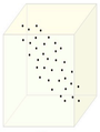
Data in original Space
-
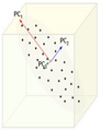
Extraction of the principal components
-
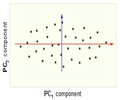
Reduction of dimensionality by keeping the first two principal components and removing the third one


Now, consider the ability of the two of the above example components (PC1 and PC2) to retain information from the original data. The data in the original space is projected onto each of these two components separately in the figures below. Notice that PC1 is better able to capture the variation in the original data than PC2. If the goal was to reduce the original d=3 dimensional data to p=1 dimension, PC1 would be preferable to PC2.

PCA Plot example
For example<ref> https://onlinecourses.science.psu.edu/stat857/sites/onlinecourses.science.psu.edu.stat857/files/lesson05/PCA_plot.gif </ref>, in the top left corner of the image below, the point [math]\displaystyle{ x_1 }[/math] is shown in a two-dimensional space and it's coordinates are [math]\displaystyle{ (x_i, 1) }[/math] and [math]\displaystyle{ (x_i, 2) }[/math]
All the red points in the plot represented by their projected values on the two original coordinators (Feature 1, Feature 2).
In PCA technique, it uses new coordinators (showed in green). As coordinate system changed, the points also are shown by their new pair of coordinate values for example [math]\displaystyle{ (z_i, 1) }[/math] and [math]\displaystyle{ (z_i, 2) }[/math]. These values are determined by original vector, and the relation between the rotated coordinates and the original ones.

In the original coordinates the two vectors [math]\displaystyle{ x_1 }[/math] and [math]\displaystyle{ x_2 }[/math] are not linearly uncorrelated. In other words, after applying PCA, if there are two principal component, and use those as the new coordinates, then it is guaranteed that the data along the two coordinates have correlation = 0
By rotating the coordinates we performed an orthonormal transform on the data. After the transform, the correlation is removed - which is the whole point of PCA.
As an example of an extreme case where all of the points lie on a straight line, which in the original coordinates system it is needed two coordinates to describe these points.
In short, after rotating the coordinates, we need only one coordinate and clearly the value on the other one is always zero. This example shows PCA's dimension reduction in an extreme case while in real world points may not fit exactly on a line, but only approximately.
PCA applications
As mentioned, PCA is a method to reduce data dimension if possible to principal components such that those PCs cover as much data variation as possible. This technique is useful in different type of applications which involve data with a huge dimension like data pre-processing, neuroscience, computer graphics, meteorology, oceanography, gene expression, economics, and finance among of all other applications.
Data usually is represented by lots of variables. In data preprocessing, PCA is a technique to select a subset of variables in order to figure our best model for data. In neuroscience, PCA used to identify the specific properties of a stimulus that increase a neuron’s probability of generating an action potential.
Figures below show some example of PCA in real world applications. Click to enlarge.
-
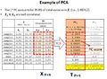
Finding two principal components of original data in 2D space. Components of data are highly correlated in original space. So they can be substituted by just one principal component, PC1, which has more than %99 of total variance of data.
-
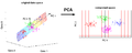
PCA in Neuroscience. Data in different classes in 3 dimensional space is mapped to a 2 dimensional space using PCA. The mapped data is clearly linearly sparable.

Tracking the useful features based on PCA:
Since in real world application, we need to know which features are important after dimensionality reduction. Then we can use those features as our new data set to continuous our project. To do this, we need to check the principal components have been chosen. Values of principal components or eigenvectors represent the weight of features within that specific principal component. Based on these weights we can tell the importance of features in the principal component. Then choose several most importance features from the original data instead of using all.
Mathematical details
PCA is a transformation from original (d-dimensional) space to a linear subspace with a new (p-dimensional) coordinate system. Each coordinate of this subspace is called a Principle Component. First principal component is the coordinate of this system along which the data points has the maximum variation. That is, if we project the data points along this coordinate, maximum variance of data is obtained (compared to any other vector in original space). Second principal component is the coordinate in the direction of the second greatest variance of the data, and so on.
For example, if we are mapping from 3 dimensional space to 2 dimensions, the first principal component is the 2 dimensional plane which has the maximum variance of data when each 3D data point is mapped to its nearest 2D point on the 2D plane.
Lets denote the basis of original space by [math]\displaystyle{ \mathbf{v_1} }[/math], [math]\displaystyle{ \mathbf{v_2} }[/math], ... , [math]\displaystyle{ \mathbf{v_d} }[/math]. Our goal is to find the principal components (coordinate of the linear subspace), denoted by [math]\displaystyle{ \mathbf{u_1} }[/math], [math]\displaystyle{ \mathbf{u_2} }[/math], ... , [math]\displaystyle{ \mathbf{u_p} }[/math] in the hope that [math]\displaystyle{ p \leq d }[/math]. First, we would like to obtain the first principal component [math]\displaystyle{ \mathbf{u_1} }[/math] or the components in the direction of maximum variance. This component can be treated as a vector in the original space and so is written as a linear combination of the basis in original space.
[math]\displaystyle{ \mathbf{u_1}=w_1\mathbf{v_1}+w_2\mathbf{v_2}+...+w_d\mathbf{v_d} }[/math]
Vector [math]\displaystyle{ \mathbf{w} }[/math] contains the weight of each basis in this combination.
[math]\displaystyle{ \mathbf{w}=\begin{bmatrix} w_1\\w_2\\w_3\\...\\w_d \end{bmatrix} }[/math]
Suppose we have n data points in the original space. We represent each data points by [math]\displaystyle{ \mathbf{x_1} }[/math], [math]\displaystyle{ \mathbf{x_2} }[/math], ..., [math]\displaystyle{ \mathbf{x_n} }[/math]. Projection of each point [math]\displaystyle{ \mathbf{x_i} }[/math] on the [math]\displaystyle{ \mathbf{u_1} }[/math] is [math]\displaystyle{ \mathbf{w}^T\mathbf{x_i} }[/math].
Let [math]\displaystyle{ \mathbf{S} }[/math] be the sample covariance matrix of data points in original space. The variance of the projected data points, denoted by [math]\displaystyle{ \Phi }[/math] is
[math]\displaystyle{ \Phi = Var(\mathbf{w}^T \mathbf{x_i}) = \mathbf{w}^T \mathbf{S} \mathbf{w} }[/math]
we would like to maximize [math]\displaystyle{ \Phi }[/math] over set of all vectors [math]\displaystyle{ \mathbf{w} }[/math] in original space. But, this problem is not yet well-defined, because for any choice of [math]\displaystyle{ \mathbf{w} }[/math], we can increase [math]\displaystyle{ \Phi }[/math] by simply multiplying [math]\displaystyle{ \mathbf{w} }[/math] by a positive scalar greater than one. And the maximum will goes to infinity which is not the proper solution for our problem. So, we add the following constraint to the problem to bound the length of vector [math]\displaystyle{ \mathbf{w} }[/math]:
[math]\displaystyle{ max_w \Phi = \mathbf{w}^T \mathbf{S} \mathbf{w} }[/math]
subject to : [math]\displaystyle{ \mathbf{w}^T \mathbf{w} =1 }[/math]
This constraint makes [math]\displaystyle{ \mathbf{w} }[/math] the unit vector in d-dimensional euclidian space and as a result the optimization problem is no longer unconstrained.
Using Lagrange Multiplier technique we have:
[math]\displaystyle{ L(\mathbf{w} , \lambda ) = \mathbf{w}^T \mathbf{S} \mathbf{w} - \lambda (\mathbf{w}^T \mathbf{w} - 1 ) }[/math]
By taking derivative of [math]\displaystyle{ L }[/math] w.r.t. primary variable [math]\displaystyle{ \mathbf{w} }[/math] we have:
[math]\displaystyle{ \frac{\partial L}{\partial \mathbf{w}}=( \mathbf{S}^T + \mathbf{S})\mathbf{w} -2\lambda\mathbf{w}= 2\mathbf{S}\mathbf{w} -2\lambda\mathbf{w}= 0 }[/math]
Note that [math]\displaystyle{ \mathbf{S} }[/math] is symmetric so [math]\displaystyle{ \mathbf{S}^T = \mathbf{S} }[/math].
From the above equation we have:
[math]\displaystyle{ \mathbf{S} \mathbf{w} = \lambda\mathbf{w} }[/math].
So [math]\displaystyle{ \mathbf{w} }[/math] is the eigenvector and [math]\displaystyle{ \lambda }[/math] is the eigenvalue of the matrix [math]\displaystyle{ \mathbf{S} }[/math] .(Taking derivative of [math]\displaystyle{ L }[/math] w.r.t. [math]\displaystyle{ \lambda }[/math] just regenerate the constraint of the optimization problem.)
By multiplying both sides of the above equation to [math]\displaystyle{ \mathbf{w}^T }[/math] and considering the constraint, we obtain:
[math]\displaystyle{ \Phi = \mathbf{w}^T \mathbf{S} \mathbf{w} = \mathbf{w}^T \lambda \mathbf{w} = \lambda \mathbf{w}^T \mathbf{w} = \lambda }[/math]
The interesting result is that objective function is equal to eigenvalue of the covariance matrix. So, to obtain the first principle component, which maximizes the objective function, we just need the eigenvector corresponding to the largest eigenvalue of [math]\displaystyle{ \mathbf{S} }[/math]. Subsequently, the second principal component is the eigenvector corresponding to the second largest eigenvalue, and so on.
Principal component extraction using singular value decomposition
Singular Value Decomposition (SVD), is a well-known way to decompose any kind of matrix [math]\displaystyle{ \mathbf{A} }[/math] (m by n) into three useful matrices.
[math]\displaystyle{ \mathbf{A} = \mathbf{U}\mathbf{\Sigma}\mathbf{V}^T }[/math].
where [math]\displaystyle{ \mathbf{U} }[/math] is m by m unitary matrix, [math]\displaystyle{ \mathbf{UU^T} = I_m }[/math], each column of [math]\displaystyle{ \mathbf{U} }[/math] is an eigenvector of [math]\displaystyle{ \mathbf{AA^T} }[/math]
[math]\displaystyle{ \mathbf{\Sigma} }[/math] is m by n diagonal matrix, non-zero elements of this matrix are square roots of eigenvalues of [math]\displaystyle{ \mathbf{AA^T} }[/math].
[math]\displaystyle{ \mathbf{V} }[/math] is n by n unitary matrix, [math]\displaystyle{ \mathbf{VV^T} = I_n }[/math], each column of [math]\displaystyle{ \mathbf{V} }[/math] is an eigenvector of [math]\displaystyle{ \mathbf{A^TA} }[/math]
Now, comparing the concepts of PCA and SVD, one may find out that we can perform PCA using SVD.
Let's construct a matrix p by n with our n data points such that each column of this matrix represent one data point in p-dimensional space:
[math]\displaystyle{ \mathbf{X} = [\mathbf{x_1} \mathbf{x_2} .... \mathbf{x_n} ] }[/math]
and make another matrix [math]\displaystyle{ \mathbf{X}^* }[/math] simply by subtracting the mean of data points from [math]\displaystyle{ \mathbf{X} }[/math].
[math]\displaystyle{ \mathbf{X}^* = \mathbf{X} - \mu_X[1, 1, ... , 1], \mu_X = \frac{1}{n} \sum_{i=1}^n x_i }[/math]
Then we will get a zero-mean version of our data points for which [math]\displaystyle{ \mathbf{X^*} \mathbf{X^{*^T}} }[/math] is the covariance matrix.
So, [math]\displaystyle{ \mathbf{\Sigma} }[/math] and [math]\displaystyle{ \mathbf{U} }[/math] give us the eigenvalues and corresponding eigenvectors of covariance matrix, respectively. We can then easily extract the desired principal components.
MATLAB example
In this example we use different pictures of a man's face with different facial expressions. But, these pictures are noisy. So the face is not easily recognizable. The data set consists of 1965 pictures each 20 by 28. So dimensionality is 20*28= 560.
Our goal is to remove noise using PCA and of course by means of SVD function in matlab. We know that noise is not the main feature that makes these pictures look different, so noise is among least variance components. We first extract the principal components and then remove those which correspond to the least values of eigenvalues of covariance matrix. Here, eigenvalues are sorted in a descending order from column to column of matrix S. For example, the first column of matrix U, which corresponds to the first element in S, is the first principal component.
We then reconstruct the picture using first d principal components. If d is too large, we can not completely remove the noise. If it is too small, we will lose some information from the original data. For example we may lose the facial expression (smile, sadness and etc.). We can change d until we achieve a reasonable balance between noise reduction and information loss.
 >> % loading the noisy data, file "noisy" stores our variable X which contains the pictures
 >> load noisy;
 >>
 >>
 >> % show a sample image in column 1 of matrix X
 >> imagesc(reshape(X(:,1),20,28)')
 >>
 >> % set the color of image to grayscale
 >> colormap gray
 >>
 >> % perform SVD, if X matrix if full rank, will obtain 560 PCs
 >> [U S V] = svd(X);
 >>
 >> d= 10;
 >>
 >> % reconstruct X using only the first d principal components and removing noise
 >> XX = U(:, 1:d)* S(1:d,1:d)*V(:,1:d)' ;
 >>
 >> % show image in column 1 of XX which is a noise reduced version
 >> imagesc(reshape(XX(:,1),20,28)')
PCA continued, Lagrange multipliers, singular value decomposition (SVD) (Lecture 2: Sept. 15, 2014)
Principal component analysis (continued)
PCA is a method to reduce dimensions in data or to extract features from data.
Given a data point in vector form [math]\displaystyle{ \,x }[/math] the goal of PCA is to map [math]\displaystyle{ \,x }[/math] to [math]\displaystyle{ \,y }[/math] where [math]\displaystyle{ \,x }[/math] [math]\displaystyle{ \,\isin }[/math] [math]\displaystyle{ \,\real }[/math]d and [math]\displaystyle{ \,y }[/math] [math]\displaystyle{ \,\isin }[/math] [math]\displaystyle{ \,\real }[/math]p such that p is much less than d. For example we could map a two-dimensional data point onto any one-dimensional vector in the original 2D space or we could map a three-dimensional data point onto any 2D plane in the original 3D space.
The transformation from d-dimensional space to p-dimensional space is chosen in such a way that maximum variance is retained in the lower dimensional subspace. This is useful because variance represents the main differences between the data points, which is exactly what we are trying to capture when we perform data visualization. For example, when taking 64-dimensional images of hand-written digits, projecting them onto 2-dimensional space using PCA captures a significant amount of the structure we care about.
-
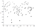
Note that the x-axis captures the value of the number, where 1s are on the left, 2s in the middle and 0s on the right. The y-axis captures tilt.

In terms of data visualization, it is fairly clear why PCA is important. High dimensional data is sometimes impossible to visualize. Even a 3D space can be fairly difficult to visualize, while a 2D space, which can be printed on a piece of paper, is much easier to visualize. If a higher dimensional dataset can be reduced to only 2 dimensions, it can be easily represented by plots and graphs.
In the case of many data points [math]\displaystyle{ \,x_i }[/math] in d-dimensional space:
[math]\displaystyle{ \,X_{dxn} = [x_1 x_2 ... x_n] }[/math]
There is an infinite amount of vectors in [math]\displaystyle{ \,\real }[/math]p to which the points in X can be mapped. When mapping these data points to lower dimensions information will be lost. To preserve as much information as possible the points are mapped to a vector in [math]\displaystyle{ \real }[/math]p which will preserve as much variation in the data as possible. In other words, the data is mapped to the vector in [math]\displaystyle{ \real }[/math]p that will have maximum variance. In the images below, the data points mapped onto u in Mapping 1 have greater variance than in Mapping 2, and thus preserves more information in the data.
-
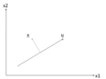
Figure 1. Two dimensional point mapped onto one dimensional vector
-
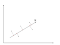
Figure 2. Mapping 1: Mapping of a two dimensional data set onto a one dimensional vector
-
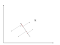
Figure 3. Mapping 2: Mapping of a two dimensional data set onto a one dimensional vector


Notice(Figure 1.) the projection of a single data point x on u is p = uTx (a scalar), thus the projection of multiple data points(Figure 2.) onto u is computed by Y = uTX, where X is the matrix representing multiple data points. The variance of Y can be calculated easily as Y is a 1 by n vector.
Expand to higher dimensional space [math]\displaystyle{ \,\real }[/math]q where q > 1, Covariance is used to find the variance of Y. The formula is given by: Var(uTX) = uTSu where S is the sample covariance matrix of X.
In finding the first principal component the objective is to find the direction u which will have the greatest variance of the points projected onto it. This can be expressed as the following optimization problem:
maxu uTSu
s.t. uTu = 1
The restriction uTu = 1 is to bound the problem. If the length of u were not restricted, uTSu would go to infinity as the magnitude of u goes to infinity. The selection of 1 as the bound is arbitrary.
Also from the three images above, we can see that the first principal component is the "line of best fit" that passes through the multi-dimensional mean of all data points, that minimizes the sum of distance squared from data points to the vector. Tho not illustrated but if the above example is doing dimensional reduction from R3 to R1, then the second principal component will have the same fashion as first component, with correlation between the first component and data points removed.
Lagrange multipliers
The Lagrange multiplier is a method for solving optimization problems. After constraining the principal component analysis output vector to an arbitrary size the task of maximizing variance in lower dimensional spaces becomes an optimization problem.
Lagrange multipler theorem
The method of Lagrange multipliers states that given the optimization problem:
   [math]\displaystyle{ max\ f(x,y) }[/math]
      [math]\displaystyle{ s.t.\ g(x,y) = c  }[/math]
The Lagrangian is defined by:
[math]\displaystyle{ \ L(x,y,\lambda)= f(x,y) - \lambda(g(x,y)-c) }[/math]
,where [math]\displaystyle{ \ \lambda }[/math] term may be either added or subtracted.
Which implies, where [math]\displaystyle{ \bigtriangledown\ }[/math] is the gradient, that:
[math]\displaystyle{ \bigtriangledown\ f(x,y) = \lambda \bigtriangledown g(x,y) }[/math]
[math]\displaystyle{ \bigtriangledown\ f(x,y) - \lambda \bigtriangledown g(x,y) = 0 }[/math]
In practice,
[math]\displaystyle{ \bigtriangledown\ L }[/math] is calculated by computing the three partial derivatives of [math]\displaystyle{ \ L }[/math] with respect to [math]\displaystyle{ \ x, y, \lambda }[/math], setting them to 0, and solving the resulting system of equations.
That is to say, the solution is given by taking the solution of:
[math]\displaystyle{ \ \bigtriangledown L = \begin{bmatrix} \frac{\partial L}{\partial x}\\\frac{\partial L}{\partial y}\\\frac{\partial L}{\partial \lambda}\end{bmatrix}= 0 }[/math]
which maximize the objective function f(x,y).
Intuitive explanation
The Lagrange multiplier utilizes gradients to find maximum values subject to constraints. A gradient [math]\displaystyle{ \bigtriangledown }[/math] is a vector which collects all of the partial derivatives of a function. Intuitively, this can be thought of as a vector which contains the slopes of all of a graph's tangent lines, or the direction which each point on the graph points.
Finding a point where the gradient of f(x,y) and g(x,y) differ by a factor lambda: [math]\displaystyle{ \bigtriangledown f(x,y) = \lambda \bigtriangledown g(x,y) }[/math] defines a point where our restraint and objective functions are both pointing in the same direction. This is important because if our objective function is pointing in a higher direction than g, increasing our objective function will increase our output, meaning we are not at a maximum. If the restraint is pointing in a higher direction than f, then reducing our input value will yield a higher output. The factor lambda is important because it is adjusted to ensure that the constraint is satisfied and maximized at our current location.
Lagrange multiplier example
Consider the function [math]\displaystyle{ \ f(x,y) = x - y }[/math] such that [math]\displaystyle{ \ g(x,y) = x^2 + y^2 = 1 }[/math]. We would like to maximize this objective function.
Calculating the Lagrangian gives
- [math]\displaystyle{ \ \text{L}(x,y,\lambda) = x - y - \lambda g(x,y) = x - y - \lambda (x^2 + y^2 - 1) }[/math]
This gives three partial derivatives:
- [math]\displaystyle{ \frac{\partial L}{\partial x} = 1 - 2\lambda x = 0, \frac{\partial L}{\partial y} = -1 - 2\lambda y = 0, \frac{\partial L}{\partial \lambda} = - (x^2 + y^2 - 1) = 0 }[/math]
This gives two solutions:
- [math]\displaystyle{ x = \frac{\sqrt{2}}{2}, y = \frac{-\sqrt{2}}{2}, \lambda = \frac{1}{\sqrt{2}} }[/math]
- [math]\displaystyle{ x = \frac{-\sqrt{2}}{2}, y = \frac{\sqrt{2}}{2}, \lambda = \frac{1}{\sqrt{2}} }[/math]
Both solutions give extreme values of our objective function. Because this is an optimization problem we are interested in the solution which gives the maximum output, which is solution 1.
Singular value decomposition revisited
Any matrix X can be decomposed to the three matrices: [math]\displaystyle{ \ U \Sigma V^T }[/math] where:
[math]\displaystyle{ \ U }[/math] is an m x m matrix of the eigenvector XXT
[math]\displaystyle{ \ \Sigma }[/math] is an m x n matrix containing singular values along the diagonal and zeroes elsewhere
[math]\displaystyle{ \ V^T }[/math] is an orthogonal transpose of a n x n matrix of the eigenvector XTX
Connection of Singular Value Decomposition to PCA
If [math]\displaystyle{ \,X }[/math] is centered (has a mean of 0) then [math]\displaystyle{ \,XX^T }[/math] is the covariance matrix.
Recall that for a square, symmetric matrix [math]\displaystyle{ \,A }[/math], we can have [math]\displaystyle{ \,A = W \Lambda W^T }[/math] where columns of [math]\displaystyle{ \,W }[/math] are eigenvectors of [math]\displaystyle{ \,A }[/math], and [math]\displaystyle{ \,\Lambda }[/math] is a diagonal matrix containing the eigenvalues.
Using the SVD of [math]\displaystyle{ \,X }[/math] we get [math]\displaystyle{ \,X=U \Sigma V^T }[/math]. Then consider [math]\displaystyle{ \,XX^T }[/math]:
[math]\displaystyle{ \ XX^T = (U \Sigma V^T)(U \Sigma V^T)^T }[/math]
[math]\displaystyle{ \ XX^T = (U \Sigma V^T)(V \Sigma U^T) }[/math]
[math]\displaystyle{ \ XX^T = U \Sigma V^T V \Sigma U^T }[/math]
[math]\displaystyle{ \ XX^T = U \Sigma I \Sigma U^T }[/math] (By the definition of V)
[math]\displaystyle{ \ XX^T = U \Sigma^2 U^T }[/math]
Thus [math]\displaystyle{ \,U }[/math] is the matrix containing eigenvectors of the covariance matrix [math]\displaystyle{ \,XX^T }[/math].
It is important to remember that [math]\displaystyle{ \,U }[/math] and [math]\displaystyle{ \,V }[/math] are unitary matricies, i.e.: [math]\displaystyle{ \, U^TU=UU^T=I }[/math] and [math]\displaystyle{ \,V^TV=VV^T=I }[/math], each equality using the appropriate dimensional identity matrix. It is also interesting that the nonsquare matrix formed by taking a subset of the eigenvectors contained in [math]\displaystyle{ \,U }[/math] or [math]\displaystyle{ \,V }[/math] has the property that [math]\displaystyle{ \,V^TV=I }[/math] (the appropriate lower dimensional identity matrix).
Matlab example of dimensionality reduction using PCA
The following example shows how principal component analysis can be used to identify between a handwritten 2 and a handwritten 3. In the example the original images are each 64 pixels and thus 64 dimensional. By reducing the dimensionality to 2D the 2's and 3's are visualized on a 2D plot and can it could be estimated as to which digit one was.
 >> % load file containing 200 handwritten 2's and 200 handwritten 3's
 >> load 2_3;
 >>
 >> who?
 >> % displays that X is 64x400 matrix containing the handwritten digits
 >>
 >> imagesc(reshape(X(:,1),8,8)')
 >> colormap gray
 >> % displays first image, a handwritten 2
 >>
 >> M = mean(X,2)*ones(1,400);
 >> Xb = X-M
 >> % M is the matrix of the mean of column vectors repeated 400 times
 >> % Xb is data centred about mean
 >>
 >> % Now use SVD to find eigenvectors, eigenvalues of Xb
 >> [U S V] = svd(Xb);
 >>
 >> % 2D projection on points
 >> Y = U(:,1:2)'*X;
 >>
 >> % 2D projections of 2's
 >> plot(Y(1,1:200),Y(2,1:200),'.')
 >>
 >> % 2D projections of 3's
 >> plot(Y(1,201:400),Y(2,201:400),'.')
PCA Algorithm, Dual PCA, and Kernel PCA (Lecture 3: Sept. 17, 2014)
PCA Algorithm (Algorithm 1)
- Recover basis
- To find the basis for PCA we first center the data by removing the mean of the sample, then calculate the covariance:
- Let [math]\displaystyle{ U }[/math] be the eigenvectors of [math]\displaystyle{ XX^T }[/math] corresponding to the top [math]\displaystyle{ \,d }[/math] eigenvalues.
- Encode training data
- To encode our data using PCA we let
- where [math]\displaystyle{ Y }[/math] is an encoded matrix of the original data
- Reconstruct training data
- To project our data back to the higher dimension
- Encode test example
- where [math]\displaystyle{ \,y }[/math] is an encoding of [math]\displaystyle{ \,x }[/math]
- Reconstruct test example
Dual principal component analysis
- Motivation
In some cases the dimension of our data can be much larger than the number of data points [math]\displaystyle{ ( d \gt \gt n ) }[/math]. For example, suppose we are interested in weekly closing rates of the Dow Jones Industrial Average, S&P 500 Index, and the NASDAQ Composite Index over the past forty years. In this example we only have three data points [math]\displaystyle{ ( n = 3 ) }[/math], but our dimension is over two thousand! [math]\displaystyle{ ( d \approx 2080 ) }[/math] Consequently, the matrix [math]\displaystyle{ XX^T }[/math] used to find the basis [math]\displaystyle{ U }[/math] is [math]\displaystyle{ 2080\times2080 }[/math], which is computationally heavy to calculate. As another example is studying genes for patients since the number of genes studied is likely much larger than the number of patients. When the data's dimensionality is high relative to the number of data points collected, a less compute-intensive way of recovering the basis is desirable. Calculating dual PCA is more efficient than PCA when the number of data points is lower relative to the dimensionality of the data. This is intuitive because it allows us to model our optimization problem as a decomposition of our data, rather than our dimensions.
- Recall from Lecture 2 how we used singular value decomposition for PCA:
- Multiply both sides by V to get:
- Since [math]\displaystyle{ V^T V = I }[/math] (the identity matrix) the SVD can be rearranged as
- Then, multiply both sides by [math]\displaystyle{ \Sigma }[/math]-1 to get:
- And so [math]\displaystyle{ U }[/math] can be calculated in terms of [math]\displaystyle{ V }[/math] and [math]\displaystyle{ \Sigma }[/math]. [math]\displaystyle{ V }[/math] is the eigenvectors of [math]\displaystyle{ X^T X_{n \times n} }[/math], so it is much easier to find than [math]\displaystyle{ U }[/math] because [math]\displaystyle{ n\lt \lt d }[/math].
- Algorithm
- We can replace all instances of [math]\displaystyle{ \,U }[/math] in Algorithm 1 with the dual form, [math]\displaystyle{ \,U = X V \Sigma^{-1} }[/math], to obtain the algorithm for Dual PCA.
- Recover Basis:
- For the basis of Dual PCA, we calculate
- then let [math]\displaystyle{ \,V }[/math] be the eigenvectors of [math]\displaystyle{ \,XX^T }[/math] with respect to the top d eigenvalues. Finally we let [math]\displaystyle{ \,\Sigma }[/math] be the diagonal matrix of square roots of the top d eigenvalues.
- Encode Training Data:
- Using Dual PCA to encode the data, let
- where [math]\displaystyle{ Y }[/math] is an encoded matrix of the original data
- Reconstruct Training Data:
- Project the data back to the higher dimension by
- Encode Test Example:
- where [math]\displaystyle{ \,y }[/math] is an encoding of [math]\displaystyle{ \,x }[/math]
- Reconstruct Test Example:
- Note that the steps of Reconstructing training data and Reconstructioning test example still depend on [math]\displaystyle{ d }[/math], and therefore still will
be impractical in the case that the original dimensionality of the data ([math]\displaystyle{ d }[/math]) is very large
Kernel Principal Component Analysis
- Kernel methods
Kernel methods are a class of algorithms used for analyzing patterns and measuring similarity. They are used for finding relations within a data set. Kernel methods map data into a higher-dimensional space to make it easier to find these relations. While PCA is designed for linear variabilities, a lot of higher-dimensional data are nonlinear. This is where Kernel PCA can be useful to help model the data variability when it comes to a nonlinear manifold. Generally speaking, Kernels is a measure of "similarity" between data points without explicitly performing the dot product between data points pairs. This can be done using different methods. For example, the dot product looks at whether vectors are orthogonal. The Gaussian kernel looks at whether two objects are similar on a scale of 0 to 1. Kernels also measure similarity between trees. We will not go in too much detail at the moment.
- Some common examples of kernels include:
- Linear kernel:
[math]\displaystyle{ \, k_{ij} = \lt x_{i},x_{j}\gt }[/math] - Polynomial kernel:
[math]\displaystyle{ \, k_{ij} = (1+\lt x_{i},x_{j}\gt )^P }[/math] - Gaussian kernel:
[math]\displaystyle{ \, k_{ij} = exp(||x_{i}-x_{j}||^2/2\sigma^2) }[/math]
Where [math]\displaystyle{ \ x_{i},x_{j} ,\isin }[/math] [math]\displaystyle{ \,\real }[/math]d
The kernel matrix [math]\displaystyle{ \, K_{n \times n} }[/math] is the matrix where [math]\displaystyle{ \, k_{ij} }[/math] is the chosen kernel between d-dimensional points [math]\displaystyle{ \ x_{i} }[/math] and [math]\displaystyle{ \ x_{j} }[/math]
- Other kernel examples can be found here:

- Kernel PCA
- With the Kernel PCA, we take the original or observed space and map it to the feature space and then map the feature space to the embedded space of a lower dimension.
- In the Kernel PCA algorithm, we can use the same argument as PCA and again use the Singular Value Decomposition (SVD) where:
- where [math]\displaystyle{ U }[/math] contains the eigenvectors of [math]\displaystyle{ \Phi(X)\Phi(X)^T }[/math]
- The goal is to reduce the dimensionality from the space X to the dimensionality of space Y by passing through H without having to know [math]\displaystyle{ \Phi(X) }[/math] exactly.
- The algorithm is similar to the Dual PCA algorithm except that the training and the test data cannot be reconstructed since [math]\displaystyle{ \Phi(X) }[/math] is unknown.
- Algorithm
- Recover Basis:
- For the basis of Kernel PCA, we calculate
- using the kernel [math]\displaystyle{ K }[/math] and let [math]\displaystyle{ V }[/math] be the eigenvectors of [math]\displaystyle{ \Phi(X)^T \Phi(X) }[/math] with respect to the top [math]\displaystyle{ p }[/math] eigenvalues. Finally we let [math]\displaystyle{ \Sigma }[/math] be the diagonal matrix of square roots of the top [math]\displaystyle{ p }[/math] eigenvalues.
- Encode Training Data:
- Using Kernel PCA to encode the data, let
- Recall [math]\displaystyle{ U = \Phi(X) V \Sigma^{-1} }[/math]:
- where [math]\displaystyle{ Y }[/math] is an encoded matrix of the image of the original data in the function [math]\displaystyle{ \Phi }[/math]. [math]\displaystyle{ Y }[/math] is computable without knowledge of [math]\displaystyle{ \Phi(X) }[/math] via the kernel function.
- Reconstruct Training Data:
- However, [math]\displaystyle{ \Phi(X) }[/math] is unknown so we cannot reconstruct the data.
- Encode Test Example:
- This is possible because we know that [math]\displaystyle{ \Phi(X)^T \Phi(X) = K(X,x) }[/math].
- Recall
- [math]\displaystyle{ U = \Phi(X) V \Sigma^{-1} }[/math]:
- [math]\displaystyle{ \Phi(X) }[/math] is the transformation of the training data [math]\displaystyle{ X_{d \times n} }[/math] while [math]\displaystyle{ \Phi(x) }[/math] is the transformation of the test example [math]\displaystyle{ x_{d \times 1} }[/math]
- Reconstruct Test Example:
- Once again, since [math]\displaystyle{ \Phi(X) }[/math] is unknown, we cannot reconstruct the data.
Centering for kernel PCA and multidimensional scaling (Lecture 4: Sept. 22, 2014)
Centering for kernel PCA
In the derivation of kernel PCA we assumed that [math]\displaystyle{ \sum_{i=1}^n\Phi(x_i)=0 }[/math] which is improbable for a random data set and an arbitrary mapping [math]\displaystyle{ \Phi }[/math]. We must be able to ensure this condition though we don't know [math]\displaystyle{ \Phi }[/math].
Let [math]\displaystyle{ \mu=\frac{1}{n}\sum_{j=1}^n\Phi(x_j) }[/math]
Define the centered transformation (not computable)
- [math]\displaystyle{ \tilde{\Phi}:x\mapsto(\Phi(x)-\mu) }[/math]
and the centered kernel (computable)
- [math]\displaystyle{ \tilde{K}:(x,y)\mapsto \tilde{\Phi}(x)^T \tilde{\Phi}(y) }[/math]
Then
- [math]\displaystyle{ \tilde{K}(x,y) = (\Phi(x)-\mu)^T (\Phi(y)-\mu)=\Phi(x)^T\Phi(y)-\mu^T\Phi(y)-\Phi(x)^T\mu+\mu^T\mu }[/math]
[math]\displaystyle{ =K(x,y)-\frac{1}{n}\sum_{j=1}^n\Phi(x_j)^T\Phi(y)-\frac{1}{n}\sum_{j=1}^n\Phi(x_j)^T\Phi(x)+\frac{1}{n^2}\sum_{j=1}^n\sum_{i=1}^n\Phi(x_j)^T\Phi(x_i) }[/math]
[math]\displaystyle{ =K(x,y)-\frac{1}{n}\sum_{j=1}^n K(x_j,x)-\frac{1}{n}\sum_{j=1}^n K(x_j,y)+\frac{1}{n^2}\sum_{j=1}^n\sum_{i=1}^n K(x_j,x_i) }[/math]
[math]\displaystyle{ =K(x,y)-\frac{1}{n}\bold{1}^TK(X,x)-\frac{1}{n}\bold{1}^TK(X,y)+\frac{1}{n^2}\bold{1}^TK(X,X)\bold{1} }[/math]
where [math]\displaystyle{ \bold{1}=([1,1,...,1]_{1\times n})^T }[/math]
Here [math]\displaystyle{ X_{d\times n} }[/math] and [math]\displaystyle{ \{x_j\}_{j=1}^n }[/math] denotes the data set matrix and elements respectively and [math]\displaystyle{ x,y }[/math] represent test elements at which the centered kernel is evaluated.
In practice, with [math]\displaystyle{ \, X = [x_1 | x_2 | ... | x_n] }[/math] as the data matrix, the Kernel Matrix, denoted by [math]\displaystyle{ K }[/math], will have elements [math]\displaystyle{ \, [K]_{ij} = K(x_i,x_j) }[/math].
We evaluate [math]\displaystyle{ \tilde{K} = K - \frac{1}{n}\bold{1}^TK-\frac{1}{n}K\bold{1}+\frac{1}{n^2}\bold{1}^TK\bold{1} }[/math], and find the eigenvectors/eigenvalues of this matrix for Kernel PCA.
Metric Multidimensional Scaling
Multidimensional Scaling (MDS) is another dimension reduction method that attempts to preserve the pair-wise distance, [math]\displaystyle{ \,d_{ij} }[/math], between data points. MDS helps with the problem of making a configuration of points in Euclidean space by using the distance information between the patterns. For example, suppose we want to map a set of points X, [math]\displaystyle{ x \in \mathbb{R}^d }[/math], to a set of points Y, [math]\displaystyle{ y \in \mathbb{R}^p }[/math]. We want to preserve the pair-wise distances such that [math]\displaystyle{ \,d(x_i, x_j) }[/math] is approximately the same as [math]\displaystyle{ \,d(y_i, y_j) }[/math].
MDS example
We can map points in 2 dimensions to points in 1 dimension by projecting the points onto a straight line:

Note that the pair-wise distances are relatively preserved. However, the triangle inequality is not preserved:
- [math]\displaystyle{ \, d(x_1,x_2)+d(x_2,x_3) \gt d(x_1, x_3) }[/math], but [math]\displaystyle{ \, d(y_1,y_2)+d(y_2,y_3) = d(y_1, y_3) }[/math]
Another example of when it's crucial to preserve the distances between data points in lower dimension space (MDS) is when dealing with "distances between cities", as shown in here
Distance matrix
Given a [math]\displaystyle{ d x n }[/math] matrix, [math]\displaystyle{ X }[/math], the distance matrix is defined by:
- [math]\displaystyle{ D^X_{n \times n} = \begin{bmatrix} d^{(X)}_{11} & d^{(X)}_{12} & ... & d^{(X)}_{1n}\\d^{(X)}_{21} & d^{(X)}_{22} & ... & d^{(X)}_{2n}\\...\\d^{(X)}_{n1} & d^{(X)}_{n2} & ... & d^{(X)}_{nn} \end{bmatrix} }[/math]
Where [math]\displaystyle{ d^{(X)}_{ij} }[/math] is defined as the euclidean distance between points [math]\displaystyle{ x_i }[/math] and [math]\displaystyle{ x_j }[/math] in [math]\displaystyle{ \mathbb{R}^d }[/math]
Important properties:
- The matrix is symmetric
- ie [math]\displaystyle{ d^{(X)}_{ij} = d^{(X)}_{ji} \; \forall \; 1 \leq i,j \leq n }[/math]
- The matrix is always non-negative
- ie [math]\displaystyle{ d^{(X)}_{ij} \ge 0 \; \forall \; 1 \leq i,j \leq n }[/math]
- The diagonal of the matrix is always 0
- ie [math]\displaystyle{ d^{(X)}_{ii}= 0 \; \forall \; 1 \leq i \leq n }[/math]
- If [math]\displaystyle{ x_i }[/math]'s don't overlap, then all elements that are not on the diagonal are positive
- Triangle inequality holds for all distance
- Triangle inequality: [math]\displaystyle{ d_{ab} + d_{bc} \gt = d_{ac} }[/math] whenever [math]\displaystyle{ a, b, c }[/math] are three different indices
Example:
For:
[math]\displaystyle{ x_1 = (0,1) }[/math]
[math]\displaystyle{ x_2 = (1,0) }[/math]
[math]\displaystyle{ x_3 = (1,1) }[/math]
Or:
- [math]\displaystyle{ X = \begin{bmatrix} 0 & 1 & 1\\1 & 0 & 1 \end{bmatrix} }[/math]
The distance matrix is:
- [math]\displaystyle{ D^X_{3 \times 3} = \begin{bmatrix} 0 & \sqrt{2} & 1\\\sqrt{2} & 0 & 1\\1 & 1 & 0 \end{bmatrix} }[/math]
For any mapping to matrix [math]\displaystyle{ Y_{p \times n} }[/math], we can calculate the corresponding distance matrix
- [math]\displaystyle{ D^Y_{n \times n} = \begin{bmatrix} d^{(Y)}_{11} & d^{(Y)}_{12} & ... & d^{(Y)}_{1n}\\d^{(Y)}_{21} & d^{(Y)}_{22} & ... & d^{(Y)}_{2n}\\...\\d^{(Y)}_{n1} & d^{(Y)}_{n2} & ... & d^{(Y)}_{nn} \end{bmatrix} }[/math]
Where [math]\displaystyle{ d^{(Y)}_{ij} }[/math] is defined as the euclidean distance between points [math]\displaystyle{ y_i }[/math] and [math]\displaystyle{ y_j }[/math] in [math]\displaystyle{ \mathbb{R}^p }[/math]
Note that a kernel matrix is a positive semidefinite matrix.
Finding the optimal Y
MDS minimizes the metric
- [math]\displaystyle{ \text{min}_Y \sum_{i=1}^n{\sum_{j=1}^n{(d_{ij}^{(X)}-d_{ij}^{(Y)})^2}} }[/math]
Where [math]\displaystyle{ d_{ij}^{(X)} = ||x_i - x_j|| }[/math], and [math]\displaystyle{ d_{ij}^{(Y)} = ||y_i - y_j|| }[/math]
The distance matrix [math]\displaystyle{ D^{(X)} }[/math] can be converted to a kernel matrix:
- [math]\displaystyle{ K = -\frac{1}{2}HD^{(X)}H }[/math]
Where [math]\displaystyle{ H = I - \frac{1}{n}ee^T }[/math] and [math]\displaystyle{ e=\begin{bmatrix} 1 \\ 1 \\ ... \\ 1 \end{bmatrix} }[/math]
Here, K is a kernel matrix implies that K is positive semi-definite, so [math]\displaystyle{ x^TKx \geq 0 }[/math] [math]\displaystyle{ \forall x }[/math]
In fact, there is a one-to-one correspondence between symmetric matrices and kernel matrices
Theorem
If [math]\displaystyle{ D^{(X)} }[/math] is a distance matrix and if [math]\displaystyle{ K=-\frac{1}{2}HD^{(X)}H }[/math], then [math]\displaystyle{ D^{(X)} }[/math] is Euclidean if and only if [math]\displaystyle{ K }[/math] is Positive Semi-Definite,
where [math]\displaystyle{ H=I-\frac{1}{n}\bold{e}\bold{e} ^T }[/math] and [math]\displaystyle{ \bold{e}=([1,1,...,1]_{1\times n})^T }[/math]
Relation between MDS and PCA
It has been shown that the goal of MDS is to obtain [math]\displaystyle{ Y }[/math] by minimizing [math]\displaystyle{ \text{min}_Y \sum_{i=1}^n{\sum_{j=1}^n{(d_{ij}^{(X)}-d_{ij}^{(Y)})^2}} }[/math]
K is positive semi-definite so it can be written as [math]\displaystyle{ K = X^TX }[/math].
Thus
- [math]\displaystyle{ \text{min}_Y \sum_{i=1}^n{\sum_{j=1}^n{(d_{ij}^{(X)}-d_{ij}^{(Y)})^2}} =\text{min}_Y(\sum_{i=1}^n\sum_{j=1}^n(x_i^Tx_j-y_i^Ty_j)^2) }[/math]
and
- [math]\displaystyle{ \text{min}_Y(\sum_{i=1}^n\sum_{j=1}^n(x_i^Tx_j-y_i^Ty_j)^2)=\text{min}_Y(\text{Tr}((X^TX-Y^TY)^2)) }[/math]
From SVD we may make the decompositions [math]\displaystyle{ \, X^TX=V\Lambda V^T }[/math] and [math]\displaystyle{ Y^TY=Q\hat{\Lambda}Q^T }[/math]
- [math]\displaystyle{ \text{min}_Y(\text{Tr}((X^TX-Y^TY)^2))=\text{min}_Y(\text{Tr}((V\Lambda V^T-Q\hat{\Lambda}Q^T)^2))=\text{min}_Y(\text{Tr}((\Lambda-V^TQ\hat{\Lambda}Q^TV)^2)) }[/math]
Let [math]\displaystyle{ G=Q^TV }[/math]
- [math]\displaystyle{ \text{min}_{G,\hat{\Lambda}}(\text{Tr}((X^TX-Y^TY)^2))=\text{min}_{G,\hat{\Lambda}}(\text{Tr}((\Lambda-G^T\hat{\Lambda}G)^2))=\text{min}_{G,\hat{\Lambda}}(\text{Tr}(\Lambda^2+G^T\hat{\Lambda}GG^T\hat{\Lambda}G-2\Lambda G^T\hat{\Lambda}G)) }[/math]
[math]\displaystyle{ =\text{min}_{G,\hat{\Lambda}}(\text{Tr}(\Lambda^2+G^T\hat{\Lambda}^2G-2\Lambda G^T\hat{\Lambda}G)) }[/math]
It can be shown that for fixed [math]\displaystyle{ \hat{\Lambda} }[/math] that the minimum over [math]\displaystyle{ G }[/math] occurs at [math]\displaystyle{ G=I }[/math], which implies that
- [math]\displaystyle{ \text{min}_{G,\hat{\Lambda}}(\text{Tr}((X^TX-Y^TY)^2))=\text{min}_{\hat{\Lambda}}(\text{Tr}(\Lambda^2-2\Lambda\hat{\Lambda}+\hat{\Lambda}^2)=\text{min}_{\hat{\Lambda}}(\text{Tr}((\Lambda-\hat{\Lambda})^2) }[/math]
Since [math]\displaystyle{ \, \Lambda }[/math] and [math]\displaystyle{ \hat{\Lambda} }[/math] are diagonal matrices containing the eigenvalues of [math]\displaystyle{ X^TX,\text{ and } Y^TY }[/math] respectively, and all said eigenvalues are positive, then the min is clearly obtained when the [math]\displaystyle{ p }[/math] nonzero diagonal elements in [math]\displaystyle{ Y^TY }[/math] are the [math]\displaystyle{ p }[/math] largest eigenvalues in [math]\displaystyle{ X^TX }[/math]
Therefore in Euclidean space, the solution of MDS is the same as that of PCA.
Approximation to MDS Algorithm <ref> http://www.cmap.polytechnique.fr/~peyre/cours/x2005signal/dimreduc_landmarks.pdf </ref>
The problem with the MDS algorithm is that the matrices [math]\displaystyle{ D^X }[/math] and [math]\displaystyle{ K }[/math] are not sparse. It is therefore expensive to compute eigen-decompositions when the number of data points is very large. To reduce the computational work required we can use Landmark Multidimensional Scaling (LMDS). LMDS is an algorithm designed to run classical MDS to embed a chosen subset of data, landmark points, and then located the remaining data points within this space given knowledge of its distance to the landmark points. The following paper has details on FastMap, MetricMap, and Landmark MDS and unifies the mathematical foundation of the three presented MDS algorithms.
ISOMAP and LLE (Lecture 5: Sept. 29, 2014)
ISOMAP
Isomap is a nonlinear dimensionality reduction method. In Multidimensional scaling we seek to find a low dimensional embedding [math]\displaystyle{ \,Y }[/math] for some high dimensional data [math]\displaystyle{ \,X }[/math], minimizing [math]\displaystyle{ \,\|D^X - D^Y\|^2 }[/math] where [math]\displaystyle{ \, D^Y }[/math] is a matrix of euclidean distances of points on [math]\displaystyle{ \,Y }[/math] (same with [math]\displaystyle{ \,D^X }[/math]). In Isomap we assume the high dimensional data in [math]\displaystyle{ X }[/math] lie on a low dimensional manifold, and we'd like to replace the euclidean distances in [math]\displaystyle{ \, D^X }[/math] with the distance on this manifold. We don't have information about this manifold, so we approximate it by forming the k-nearest-neighbour graph between points in the dataset. The distance on the manifold can then be approximated by the shortest path between points. This is called the geodesic distance, which is a generalization of the notion of straight line to curved spaces and is denoted by [math]\displaystyle{ \, D^G }[/math]. This is useful because it allows for nonlinear patterns to be accounted for in the lower dimensional space. From this point, the rest of the algorithm is the same as MDS. The approach of Isomap is capable of discovering nonlinear degrees of freedom that underlie the complex nature of the data. This algorithm efficiently computes a globally optimal solution which is guaranteed to converge asymptotically to the true underlying structure. (Further Reading: A Global Geometric Framework for Nonlinear Dimensionality Reduction, by Joshua B. Tenenbaum, Vin de Silva, John C. Langford)
The Isomap Algorithm can thus be described through the following steps:
1. Construct the Neighbourhood Graph
Determine which points are neighbours on manifold M based on distances [math]\displaystyle{ d_{i,j}^{(X)} }[/math] between pairs of points i and j in the input space X. To do this, we can use one of the two methods below:
a) K-Nearest Neighbours: For each point i, select the k points with the minimum distance to point i as neighbours.
b) [math]\displaystyle{ {\epsilon} }[/math]-Radius Neighbourhood: For each point i, the set of neighbours is given by [math]\displaystyle{ \, \{ j : d_{i,j}^{ (X) } \lt \epsilon \} }[/math]
The neighbourhood relations are represented as a weighted graph G over the data points, with edges of weight [math]\displaystyle{ d_{i,j}^{(X)} }[/math] between the neighbouring points.
2. Compute shortest paths
Estimate geodesic distances [math]\displaystyle{ d_{i,j}^{(M)} }[/math] between all pairs of points on the manifold M by computing their shortest path distance [math]\displaystyle{ d_{i,j}^{(G)} }[/math] in graph G.
3. Construct low dimensional embeddings (classical MDS)
Apply classical MDS to the matrix of graph distances [math]\displaystyle{ D_{G} = \{ d_{i,j}^{(G)} \} }[/math], constructing an embedding of the data in a d-dimensional Euclidean space Y that best represents the manifolds estimated intrinsic geometry.
It is worth noting that as [math]\displaystyle{ D^{G} }[/math] is not a Euclidean distance, the matrix [math]\displaystyle{ K = -\frac{1}{2}HD^{(G)}H }[/math] is not guaranteed to be positive semi-definite. This is handled in the implementation [5] by considering only the positive value of the real part only, which can be considered as projecting the matrix onto the
cone of nearest positive semi-definite matrix.
It is important to note that k determines "locality". Isomap captures local structure and "unfolds" the manifold.
The swiss roll manifold is a commonly discussed example of this. Note that the Euclidean distance between points A and B drastically differs from the Geodesic distance.

ISOMAP Results
A Global Geometric Framework for Nonlinear Dimensionality Reduction is the paper that proposed ISOMAP, the below figures show some images for ISOMAP results. The first image shows the different orientation of the face images dataset, as shown in the figure the x axis captures the horizontal orientation, while the y axis captures the vertical orientation and the bar captures the lightning direction. The second image shows the 2 handwritten digits and ISOMAP results in this dataset.


Locally Linear Embedding (LLE)
Locally Linear Embedding (LLE) is another technique for nonlinear dimensionality reduction that tries to find a mapping from high dimensional space to low dimensional space such that local distances between points are preserved. LLE has some advantages over Isomap, including faster optimization and better result in many problems. LLE reconstructs each point based on its k-nearest neighbour.
E.g. [math]\displaystyle{ x_i \approx w_1x_{1}+w_2x_{2}+...+w_kx_{k} , \sum_i w_i = 1 }[/math]
-
k-nearest neighbours for x, k = 6
The method optimizes the equation [math]\displaystyle{ \mathbf{x_i-w_1x_{i1}+w_2x_{i2}+...+w_kx_{ik}} }[/math] for each [math]\displaystyle{ x_i \in X }[/math] with corresponding k-th nearest neighbour set [math]\displaystyle{ \mathbf{\, {x_{i1},x_{i2},...,x_{ik}}} }[/math]. LLE is therefore an optimization problem for:
Algorithm
- Find the k-nearest neighbour for each data point
- Compute [math]\displaystyle{ \mathbf{W_{nxn}} }[/math] through [math]\displaystyle{ \mathbf{\text{min}_W \sum_{i=1}^n{(x_i-\sum_{j=1}^n{W_{ij}x_j)^2}}} }[/math] such that [math]\displaystyle{ \mathbf{\sum w_{ij} = 1} }[/math] (which means that it's convex optimization of the points) where [math]\displaystyle{ \mathbf{x_j} }[/math] are the k-nearest neighbours of [math]\displaystyle{ \mathbf{x_i} }[/math]
- Let [math]\displaystyle{ \mathbf{V_i = [x_j | x_j} }[/math] is a neighbour of [math]\displaystyle{ \mathbf{ x_i ]_{dxk}} }[/math] Let [math]\displaystyle{ \mathbf{w(i)} }[/math] be all k weights of point [math]\displaystyle{ \mathbf{x_i} }[/math] (ie row i of W with all zeroes removed) Then:
- and hence we need to optimize
- This is a separable optimization problem which can be solved for each point independently, which can be simplified to
- Now we have
- Let [math]\displaystyle{ \mathbf{\, G =(x_ie^T-V_i)^T(x_ie^T-V_i) } }[/math]. Therefore we can instead simplify
- Use Lagrange Multipliers to optimize the above equation:
- [math]\displaystyle{ \mathbf{\frac{\partial L}{\partial {w(i)}}=2Gw(i)-\lambda e=0 } }[/math] which implies [math]\displaystyle{ \mathbf{ Gw(i)=\frac{\lambda}{2}e} }[/math] and hence [math]\displaystyle{ \mathbf{ w(i)=\frac{\lambda}{2}G^{-1}e } }[/math]
- Note that we do not need to compute [math]\displaystyle{ \mathbf{\lambda} }[/math], but can just compute [math]\displaystyle{ \mathbf{\, G^{-1}e} }[/math], then re-scale so [math]\displaystyle{ \mathbf{\, w(i)^Te=1} }[/math]
- Finally, solve [math]\displaystyle{ \mathbf{\text{min}_Y \sum_{i=1}^n{(y_i-\sum_{j=1}^t{w_{ij}y_j)^2}}} }[/math] where w is known and y is unknown
Notes:
[math]\displaystyle{ \, G_{d*d} }[/math] is invertible under some conditions depending on [math]\displaystyle{ \, k }[/math], as it must have rank [math]\displaystyle{ \, d }[/math] so [math]\displaystyle{ \, k }[/math] must be greater than or equal [math]\displaystyle{ \, d }[/math]
LLE doesn't work for out of sample case there are extensions for it to handle this as in this [6]
If we want to reduce the dimensionality to p, we need to choose the p+1 smallest eigenvectors.
Pros of Isomap:
- Calculation is based on eigenvalue and eigenvectors, thus overall stability and optimality is maintained.
- Only need one pre-determined parameter: k(nearest neighbours) or [math]\displaystyle{ \, {\epsilon} }[/math] (neighbourhood radius)
- Able to determine intrinsic dimension of signal from residual.
Cons of Isomap
- It is slow - it requires comparing all possible paths between each N(N-1)/2 pairs of points and determining which is shortest. (But this can be fixed via the Nystrom approximation which we will see later.)
- It is not obvious how to handle out of sample data
Pros of LLE:
- LLE is capable of retain the structure and characterstic of original data.
- LLE requires little parameters to calculate
- Combining 1 & 2, LLE is good for trouble shooting and error dignostics, since it can retain most from original data and needs minimal amount of parameter to calculate.
- Much faster than ISOMAP, often with comparable or better performance
Cons of LLE
- It is not obvious how to handle out of sample data
- There is no way of knowing if reducing the data to p dimensions is the optimal reduction.
LLE continued, introduction to maximum variance unfolding (MVU) (Lecture 6: Oct. 1, 2014)
LLE
Recall the steps of LLE can be summarized as follows:
- For each data point, find its [math]\displaystyle{ k }[/math] nearest neighbours for some fixed [math]\displaystyle{ k }[/math].
- Find reconstruction weights [math]\displaystyle{ W }[/math], minimizing
[math]\displaystyle{ \sum_{i=1}^n ||x_i - \sum_{j=1}^n w_{ij}x_j||^2, where \sum_j w_{ij} = 1 }[/math] - Reconstruct the low dimensional embedding with respect to these weights.
That is, find low dimensional [math]\displaystyle{ Y }[/math] minimizing
[math]\displaystyle{ \sum_{i=1}^n||y_i - \sum_{j=1}^nw_{ij}y_j||^2 }[/math].
The previous lecture covered how to find the weights [math]\displaystyle{ W }[/math]. Here we will discuss how to find the low-dimensional embedding [math]\displaystyle{ Y }[/math] using these weights.
First, we want to write the previous equation in a matrix form.
Consider that [math]\displaystyle{ Y }[/math] is a [math]\displaystyle{ p*n }[/math] matrix and [math]\displaystyle{ I_{:i} }[/math] is the [math]\displaystyle{ i^{th} }[/math] column ([math]\displaystyle{ n*1 }[/math]) in the identity matrix (like Matlab notation)
Then the sample, [math]\displaystyle{ i }[/math], can be represented as follows: [math]\displaystyle{ y_i = Y * I_{:i} = \begin{bmatrix} y_1, y_2 ,... y_i,..., y_n \end{bmatrix} \begin{bmatrix} 0 \\0 \\... \\ 1 \\ ... \\0 \end{bmatrix} }[/math]
Note that: [math]\displaystyle{ I_{i:} Y^T = y_i^T }[/math] where [math]\displaystyle{ I_{i:} }[/math] is the [math]\displaystyle{ i^{th} }[/math] row from the identity matrix
Similarly, [math]\displaystyle{ \sum w_{ij} y_i = W_{i:} Y^T }[/math]
So the objective is equivalent to minimizing [math]\displaystyle{ \sum_{i=1}^n||I_{i:} Y^T - W_{i:}Y^T||^2 = ||IY^T - WY^T||^2 }[/math]
But first, to prevent the trivial solution of the 0-matrix, we add the constraint that [math]\displaystyle{ \frac{1}{n}Y^TY = I }[/math]. Now, the objective can be rewritten as minimizing:
- [math]\displaystyle{ ||Y^T - WY^T||^2_F }[/math]
where the above norm is the Frobenius norm, which takes the square root of the sum of squares of all the entries in the matrix. Recall this norm can be written in terms of the trace operator:
- [math]\displaystyle{ ||Y^T - WY^T||^2_F = ||Y^T (I - W)||^2_F = Tr((Y^T (I - W)) (Y^T (I - W))^T)= Tr(Y^T(I-W)(I-W)^TY) }[/math]
By letting [math]\displaystyle{ \, M=(I-W)(I-W)^T }[/math], the objective function will become
- [math]\displaystyle{ \, \min_Y Tr(Y^T M Y) }[/math]
This minimization has a well-known solution: We can set the rows of [math]\displaystyle{ Y }[/math] to be the [math]\displaystyle{ d }[/math] lowest eigenvectors of [math]\displaystyle{ M }[/math], where [math]\displaystyle{ d }[/math] is the dimension of the reduced space.
To solve this minimization using the Lagrange multiplier, the Lagrangian is:
[math]\displaystyle{ L(Y, \Lambda) = Tr(Y^TMY) - Tr(\Lambda (\frac{1}{n} Y^T Y - I))) }[/math]
[math]\displaystyle{ \frac{d}{dy} L(Y, \Lambda) = 2MY- \Lambda \frac{2}{n} Y }[/math]
Setting this equal to zero and solving gives
- [math]\displaystyle{ MY = \frac{1}{n} \Lambda Y }[/math]
- [math]\displaystyle{ MY = \Lambda^* Y }[/math]
where [math]\displaystyle{ \Lambda = \begin{bmatrix} \lambda_1 & \ldots & 0 \\ 0 & \lambda_2 & \ldots\\ \vdots & \ddots & \vdots\\ 0 &\ldots & \lambda_p \end{bmatrix} }[/math]
If we want to reduce the dimensions to p, we need to choose p + 1 smallest eigenvectors. This is because the first eigenvalue of the matrix is equal to 1 since it is a Laplacian (the number of [math]\displaystyle{ 0 }[/math] eigenvalues of a Laplacian is the number of connected components).
Note that for LLE, the bottom d+1 eigenvectors of the matrix M represents a free translation mode of eigenvalue 0. By discarding this eigenvector, we enforce the constraint of [math]\displaystyle{ \sum_{i=1}^n = y_i=0 }[/math] since it means that the components of the other eigenvectors must sum to 0, because of orthogonality. The remaining d eigenvectors form the d embedding coordinates found by LLE.
Comparison between Dimensionality Reduction Approaches (Unified Framework)
| Approach | Solution \ Eigenvectors of |
|---|---|
| PCA | [math]\displaystyle{ \boldsymbol{ X^T X } }[/math] or [math]\displaystyle{ \boldsymbol{ \Sigma V^T } }[/math] |
| MDS | [math]\displaystyle{ \boldsymbol{ - \frac{1}{2} (I - \frac{1}{n} e e^T) D (I - \frac{1}{n} e e^T) } }[/math] a.k.a. [math]\displaystyle{ \boldsymbol{-\frac{1}{2} H D H} }[/math] where [math]\displaystyle{ \boldsymbol{H=(I - \frac{1}{n} e e^T)} }[/math] |
| ISOMAP | [math]\displaystyle{ \boldsymbol{ - \frac{1}{2} (I - \frac{1}{n} e e^T) D^G (I - \frac{1}{n} e e^T) } }[/math] |
| LLE | [math]\displaystyle{ \boldsymbol{ (I - W)(I - W)^T } }[/math] or [math]\displaystyle{ \boldsymbol{ \lambda I - (I - W)(I - W)^T } }[/math] |
| KPCA | [math]\displaystyle{ \boldsymbol{K} }[/math] |
From the above table we can interpret all of these algorithms as variations of kernel PCA. More details are presented in this paper: A kernel view of the dimensionality reduction of manifolds.
Note that PCA, MDS, ISOMAP and KPCA choose the largest eigenvalue/eigenvector pairs for embedding while LLE chooses the smallest pair(For MDS, D is Euclidean distance). However, in LLE, if we let [math]\displaystyle{ \lambda_{max} }[/math] be the largest eigenvalue of [math]\displaystyle{ \mathbf{L = (I-W)^T(I-W)} }[/math] and replace the matrix [math]\displaystyle{ \mathbf{ (I - W)(I - W)^T } }[/math] with [math]\displaystyle{ \mathbf{ \lambda_{max}I - (I - W)(I - W)^T } }[/math], the largest eigenvalue/eigenvector pairs will be chosen instead.
Relationship between LLE and Kernel PCA on LLE kernel
The smallest eigenvalue of LLE Kernel [math]\displaystyle{ \,(I-W)^T(I-W) }[/math] is 0. The eigenvector corresponding to this eigenvalue is [math]\displaystyle{ \,c[1,1,1,....1,1,1] }[/math].
So when we do LLE we find eigenvectors corresponding to smallest p+1 eigenvalues and discard the first eigenvector which is [math]\displaystyle{ \,c[1,1,1,....1,1,1] }[/math].
Now, If we construct a new matrix, a so-called deflated matrix by multiplying [math]\displaystyle{ \,\Phi(x)=I-W }[/math] with a factor [math]\displaystyle{ \,(I-\frac{1}{n}ee^T) }[/math], we will get a new kernel with rank d-1.
i.e. [math]\displaystyle{ \,\hat{K} = \hat{\phi(x)}^T \hat{\phi(x)} = (I-\frac{1}{n}ee^T)K(I-\frac{1}{n}ee^T) }[/math] has the eigenvector [math]\displaystyle{ \,c[1,1,1,....1,1,1] }[/math] removed.
Next we only need to find eigenvectors corresponding to smallest p eigenvalues and do not need to discard the first one, since it has been moved already.
However, we realize that [math]\displaystyle{ \,(I-\frac{1}{n}ee^T) }[/math] equals the centering matrix [math]\displaystyle{ \,H }[/math].
So what we do in LLE is similar to what we do in Kernel PCA.
In fact doing LLE is equivalent to perform Kernel PCA on LLE kernel up to a scaling factor.
Supervised Locally Linear Embedding
Dick et al (2003) proposed a supervised LLE. The big difference between LLE and SLLE is that in SLLE, the class information of data would be considered to get the nearest neighbors.
Maximum variance unfolding
In maximum variance unfolding (MVU), as in isomap and LLE, we try to reduce the dimensionality of a nonlinear data. We may assume that the data is sampled from a low-dimensional manifold that is embedded within a higher-dimensional Euclidean space. The aim is to "unfold" this manifold in a lower-dimensional Euclidean space such that the local structure of each point is preserved. We would like to preserve the distance from any point to each of its [math]\displaystyle{ k }[/math] nearest neighbours, while maximizing the pairwise variance for all points which are not its neighbours. The MVU algorithm uses semidefinite programming to find such a kernel.
Optimization constraints
For a kernel [math]\displaystyle{ \Phi }[/math] such that [math]\displaystyle{ x \mapsto \phi(x) }[/math], we have the following 3 constraints:
- [math]\displaystyle{ \Phi }[/math] must be centred, i.e. [math]\displaystyle{ \sum\limits_{i,j} k_{ij} = 0 }[/math].
- [math]\displaystyle{ k }[/math] should be positive semi-definite, i.e. [math]\displaystyle{ k \succeq 0 }[/math].
- The local distance should be maintained between data and its embedding.
This means that for [math]\displaystyle{ i, j }[/math] such that [math]\displaystyle{ x_i, x_j }[/math] are neighbours, we require that [math]\displaystyle{ \Phi }[/math] satisfies
[math]\displaystyle{ \, | x_i - x_j |^2 = |\phi(x_i) - \phi(x_j)|^2 }[/math]
[math]\displaystyle{ \, = [\phi(x_i) - \phi(x_j)]^T [\phi(x_i) - \phi(x_j)] }[/math]
[math]\displaystyle{ \, =\phi(x_i)^T \phi(x_i) - \phi(x_i)^T \phi(x_j) - \phi(x_j)^T \phi(x_i) + \phi(x_j)^T \phi(x_j) }[/math]
[math]\displaystyle{ \, =k_{ii} - k_{ij} - k_{ji} + k_{jj} }[/math]
[math]\displaystyle{ \, =k_{ii} -2k_{ij} + k_{jj} }[/math]
where [math]\displaystyle{ \, K=\phi^T \phi }[/math] is the [math]\displaystyle{ n \times n }[/math] kernel matrix.
We can summarize this third constraint as:
[math]\displaystyle{ \, n_{ij} ||x_i - x_j||^2 = n_{ij} || \phi(x_i) - \phi(x_J) ||^2 }[/math]
where [math]\displaystyle{ n_{ij} }[/math] is the neighbourhood indicator, that is, [math]\displaystyle{ n_{ij} = 1 }[/math] if [math]\displaystyle{ x_i, x_j }[/math] are neighbours and [math]\displaystyle{ 0 }[/math] otherwise.
Optimization problem
One option for finding the correct K would be to minimize the rank of K. The intuition behind this is that even though the data might be high-dimensional, it lies on a manifold of low dimension. Since [math]\displaystyle{ rank }[/math] is not a convex function, the objective function is ill-defined and is replaced with [math]\displaystyle{ Tr(K), }[/math] since when K is semidefinite the trace is just equal to the sum of the singular values. However, in practice minimizing the trace does not result in a faithful low-dimensional representation. An explanation for this phenomenon is still an open problem.
Recall that in PCA, [math]\displaystyle{ Var(X) = \boldsymbol{\lambda}_1 + \boldsymbol{\lambda}_2 + \cdots + \boldsymbol{\lambda}_d = Tr(S) }[/math]. To find a useful K, the objective of [math]\displaystyle{ Tr(K) }[/math] can still be used, but the problem has to be changed from a minimization to a maximization. The intuition here is that you are maximizing the total variance explained by the kernel. Thus the problem is
- [math]\displaystyle{ \text{max } Tr(K) }[/math]
- [math]\displaystyle{ \text{subject to above constraints} }[/math]
which is a semidefinite program.
MVU (Maximum Variance Unfolding) Method
- Construct the neighbourhood graph using k-nearest neighbours
- Find the kernel K by solving the SDP problem: max [math]\displaystyle{ Tr(K) }[/math] such that
[math]\displaystyle{ K_{ii}+K_{jj}-2K_{ij} = D_{ij}, \sum_{ij} K_{ij} = 0, K \succeq 0 }[/math] - Apply Kernel PCA on the learned kernel K
Maximum Variance Unfolding is a useful non-linear interpretation of the PCA intuition. MVU is robust and will preserve the nearest neighbours of the original data in any mapping.
To categorize dimension reduction methods we have learnt so far
| Locality Preserving methods | Globality Preserving methods | |
|---|---|---|
| Linear methods | LLE | MDS, PCA |
| Non-linear methods | ISOMAP, LPP(locality preserving projection) | MVU, KPCA |
Action Respecting Embedding and Spectral Clustering (Lecture 7: Oct. 6, 2014)
SDE Paper Notes
Unsupervised Learning of Image Manifolds by Semidefinite Programming introduced the maximum variance unfolding technique. The results of the paper compare the proposed technique against existing dimensionality reduction techniques. The first figure compares SDE against PCA in the "faces" dataset. To maintain the entire dataset variation we need 5 dimensions using SDE, while we need 10 dimensions using PCA. The second figure compares SDE against ISOMAP in a non-convex dataset. To maintain the whole dataset variation we need only 2 dimensions using SDE, while we need more than 5 dimensions using ISOMAP. The two figures show that SDE can represent data variation using a much smaller number of eigenvectors than PCA or ISOMAP. Also, if two points take the same action, the distance between theses two points should not change( this is important ). Rotation and transaction matrix are the only way to remain the distance.
-
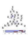
Results of SDE against PCA. The figure is taken from here
-
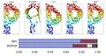
Results of SDE against ISOMAP. The figure is taken from here


SDE against ISOMAP showcases a known problem that ISOMAP can struggle against non-convex data.
Action Respecting Embedding
When we are dealing with temporal data (data in which the order is important) we could consider a technique called Action Respecting Embedding. Examples include stock prices, which are time series, or a robot that moves around and takes pictures at different positions. Usually there are various actions that transform one data point into the next data point. For example, consider a robot taking pictures at different positions: actions include stepping forward, stepping backward, stepping right, turning, etc. After each action, the robot takes a picture at its current position, then undertakes another action, continuing until a set of data points is collected. Or consider a financial time series, where actions include stock splits, interest rate reduction, etc. Or consider a patient under a treatment, where actions include taking a specific step in the treatment or taking a specific drug, which could affect blood sugar level, cholesterol, etc.
Some information cannot be captured in the form of similarities.
Action Respecting Embedding takes a set of data points [math]\displaystyle{ \, x_{1},...,x_{n} }[/math] along with associated discrete actions [math]\displaystyle{ \, a_{1},...,a_{n-1} }[/math]. The data points are assumed to be in temporal order, where [math]\displaystyle{ \, a_{i} }[/math] was taken between [math]\displaystyle{ \ x_{i} }[/math] and [math]\displaystyle{ \ x_{i+1} }[/math].
Contain all actions to be distance preserving transformations in the feature space.
Now we realize that intuitively, if two points have the same action, then the distance between them should not change after the action. There are only three types of transformations that do not change the distance between points. They are rotation, reflection, and translation. Since rotation and reflection have the same properties, we will call both of these rotation for our purposes. Any other transformation does not preserve distances. Note that we are able to model any action in low dimensional space by rotation, translation or any affine combination of them.
Action Respecting Embedding has similar algorithm to SDE[7]
Algorithm
1) Construct a neighbourhood representation
2) Solve to find maximum variance subject to constraints
3) Construct lower dimensional embedding from eigenvectors of the kernel
Differences:
1) Constructing neighbourhoods based on action pairs
2) Adding action constraints
Optimization Problem
Recall that kernel function satisfies the property: [math]\displaystyle{ \, |\phi(x_i) - \phi(x_j)|^2 = | x_i - x_j |^2 }[/math].
We can formulate the idea of distance preserving mathematically as [math]\displaystyle{ \, |\phi(x_i) - \phi(x_j)|^2 = |\phi(x_i+1) - \phi(x_j+1)|^2 }[/math], if [math]\displaystyle{ \, x_i, x_j }[/math] are points that perform the same type of transformations.
The maximum variance unfolding problem is
- ,such that
[math]\displaystyle{ \sum\limits_{i,j} k_{ij} = 0 }[/math]
[math]\displaystyle{ k \succeq 0 }[/math]The Action Respecting Embedding problem is similar to the maximum variance unfolding problem, with another constraint:
For all i, j, [math]\displaystyle{ a_{i} = a_{j} }[/math],
A Simple Example
Consider the two examples presented in the ARE paper [8] of a robot moving around taking pictures with some action between them. The input is a series of pictures with actions between them. Note that there are no semantics for the actions, only labels
The first example is a robot that takes 40 steps forward then takes a 20 steps backward. The following figure (which is taken from ARE paper [9] shows the action taking by the robot and the results of ARE and SDE. We can see that ARE captures the trajectory of the robot. Although ARE doesn't have semantics for each action it captured an essential property of these actions that they are opposite in direction and equal in magnitude. We could look at the position on manifold vs. time for a robot that took 40 steps forward and 20 steps backward. We could also look at the same analysis for a robot that took 40 steps forward and 20 steps backward that are twice as big.
-
Action taken by robot
-
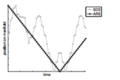
Results by ARE and SDE

Another complicated action and the result of ARE and SDE are shown in the next figure (taken from ARE paper [10]), where we can see that ARE captured the trajectory of the robot.
-
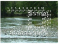
Action taken by robot
-
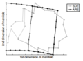
Results by ARE and SDE


Sometimes it's very hard for humans to recognize what happened by merely looking at the data, but this algorithm will make it easier for you to see exactly what happened.
Types of Applications
Action-respecting embeddings are very useful for many AI applications, especially those that involve robotics, because actions can be defined as simple transformations that are easy to understand. Another common type of application is planning, that is, when we need to find a sequence of decisions which achieve a desired goal, e.g. coming up with an optimal sequence of actions to get from one point to another.
For example, what type of treatment should I give a patient in order to get from a particular state to a desired state?
For each action [math]\displaystyle{ a }[/math], we have a collection of data points [math]\displaystyle{ \, (y_{t},y_{t+1}) }[/math] such that [math]\displaystyle{ \, y_{t} \to y_{t+1} }[/math].
Through the algorithm, we learn [math]\displaystyle{ \, f_{a} }[/math]: [math]\displaystyle{ \, f_{a}(y_{t}) = A_{a}y_{t} + b_{a} = y_{t+1} }[/math] where [math]\displaystyle{ A_{a} }[/math] is that rotation matrix for action [math]\displaystyle{ a }[/math], and [math]\displaystyle{ b_{a} }[/math] is the translation vector vector for action [math]\displaystyle{ a }[/math]. We can estimate [math]\displaystyle{ A_{a} }[/math] and [math]\displaystyle{ b_{a} }[/math]. These can be solved in closed form so that we will know what happens to any input [math]\displaystyle{ (y_t) }[/math] if action [math]\displaystyle{ a }[/math] is taken.
Spectral Clustering
Clustering is the task of grouping data such that elements in the same group are more similar (or dissimilar) to each other compared to the elements in other groups. In spectral clustering, we represent the data as a graph first and then perform clustering.
For the time being, we will only consider the case where there are two clusters.
Given [math]\displaystyle{ \{x_i\}^{n}_{i=1} }[/math] and notation of similarity or dissimilarity, we can represent the data as a weight undirected graph [math]\displaystyle{ \,G=(V,E) }[/math] where V represents the vertices (the data) and E represents the edges (similarity or dissimilarity between two data - for now we will assume simliarity).
Using intuition, we can see that the goal is to minimize the sum of the weights of the edges that we cut (i.e. edges we remove from G until we have a disconnected graph)
where A and B are the partitions of the vertices in G made by a cut, and [math]\displaystyle{ \,w_{ij} }[/math] is the weight between points i and j.
Consider the following graphs of data:
-
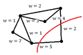
Example 1: A poor cut resulting in a sum of weights of 7
-
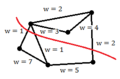
Example 2: A good cut resulting in a sum of weights of 4
-
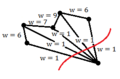
Example 3: A good cut despite having many edges cut


Although "cut" may minimize the edge weights that we use to partition, note that using cut(A,B) may cause many edges to be cut, but which have smaller weights. For example, if there is one datum that is very dissimilar to the rest of the data, we may end up partitioning this one point to itself despite it resulting in many edges being cut. This is the case in Example 3 above. This occurrence may cause an imbalance in partition sizes. To avoid this problem, we minimize the ratio-cut.
We define ratio-cut as: [math]\displaystyle{ ratiocut = \frac{cut(A, \bar{A})}{|A|} + \frac{cut(\bar{A}, A)}{|\bar{A}|} }[/math] where [math]\displaystyle{ \, |A| }[/math] is the cardinality of the set [math]\displaystyle{ \, A }[/math] and [math]\displaystyle{ \, \bar{A} }[/math] is the complement of [math]\displaystyle{ \, A }[/math].
This equation will be minimized if there is a balance between set [math]\displaystyle{ \, A }[/math] and [math]\displaystyle{ \bar{A} }[/math]. This, however, is an NP Hard problem; we must relax the constraints to arrive at a computationally feasible solution.
Let [math]\displaystyle{ f \in \mathbb{R}^n }[/math] such that
[math]\displaystyle{ f_{i} = \left\{ \begin{array}{lr} \sqrt{\frac{|\bar{A}|}{|A|}} & i \in A\\ -\sqrt{\frac{|A|}{|\bar{A}|}} & i \in \bar{A} \end{array} \right. }[/math]
We will show in the next lecture that minimizing [math]\displaystyle{ \, \sum_{ij}w_{ij}(f_{i}-f_{j})^2 }[/math] is equivalent to minimizing the ratio-cut.
Choices of [math]\displaystyle{ W }[/math]
The [math]\displaystyle{ \epsilon }[/math]-neighbourhood graph
If the pairwise distance are smaller than [math]\displaystyle{ \epsilon }[/math] between two points [math]\displaystyle{ i, j }[/math], let [math]\displaystyle{ w_{ij}=1 }[/math], else let [math]\displaystyle{ w_(i,j)=0 }[/math]. This similarity graph is generally considered an unweighted graph.
The [math]\displaystyle{ k }[/math]-nearest neighbourhood graph
If the [math]\displaystyle{ v_j }[/math] is among the [math]\displaystyle{ k }[/math]-nearest neighbours [math]\displaystyle{ v_i }[/math], then [math]\displaystyle{ w_{ij}=1 }[/math]. This will result in a non-symmetric matrix, so we can either let
- [math]\displaystyle{ w_{ij}=w_{ij}=1 }[/math] as long as [math]\displaystyle{ v_j }[/math] is among the [math]\displaystyle{ k }[/math]-nearest neighbour of [math]\displaystyle{ v_i }[/math] or [math]\displaystyle{ v_i }[/math] is among the [math]\displaystyle{ k }[/math]-nearest neighbour of [math]\displaystyle{ v_j }[/math]; or let
- [math]\displaystyle{ w_{ij}=w_{ij}=1 }[/math] only when [math]\displaystyle{ v_j }[/math] is among the [math]\displaystyle{ k }[/math]-nearest neighbour of [math]\displaystyle{ v_i }[/math] and [math]\displaystyle{ v_i }[/math] is among the [math]\displaystyle{ k }[/math]-nearest neighbour of [math]\displaystyle{ v_j }[/math].
The resulting matrix is symmetric.
The fully connected graph
As the graph is fully connected, the weight function should reflect the local neighbourhood relationships. A Gaussian similarity function is often chosen in this case.
Spectral Clustering (Lecture 8: Oct. 8, 2014)
Problem Formulation and Notations
Once we are given a set of points [math]\displaystyle{ \, x_{1},...,x_{n} }[/math] and a sense of what it is to be similar or dissimilar, we can represent these data points as a weighted undirected graph. Let [math]\displaystyle{ \, G=( V, E) }[/math] be a graph, where V is the set of vertices and E is the set of edges.
In graph theory, partitioning the set of vertices of a graph into two disjoint sets is called a cut. Consequently the set of edges which has one end point in each subset (partition) is called a cut-set, which crosses the cut. In a connected graph each cut-set determines a unique cut. So, in some cases cuts are identified with their cut-sets rather than with their vertex partitions.
The cut [math]\displaystyle{ \, C = ( A, B ) }[/math] partitions [math]\displaystyle{ \, V }[/math] from [math]\displaystyle{ \, G }[/math] into two subsets [math]\displaystyle{ A }[/math] and [math]\displaystyle{ B }[/math].
The cut-set of a cut [math]\displaystyle{ \, C = ( A, B ) }[/math] is the set [math]\displaystyle{ \{ ( i,j ) \in E | i \in A, j \in B \} }[/math] of edges that have one endpoint in [math]\displaystyle{ A }[/math] and the other endpoint in [math]\displaystyle{ B }[/math]. If [math]\displaystyle{ i }[/math] and [math]\displaystyle{ j }[/math] are specified vertices of the graph [math]\displaystyle{ G }[/math], an [math]\displaystyle{ i }[/math] [math]\displaystyle{ - }[/math] [math]\displaystyle{ j }[/math] cut is a cut in which [math]\displaystyle{ i }[/math] belongs to the set [math]\displaystyle{ A }[/math] , and [math]\displaystyle{ j }[/math] belongs to the set [math]\displaystyle{ B }[/math].
The weight of a cut is different for different types of graphs:
- In an Unweighted Undirected graph, the size or weight of a cut is the number of edges crossing the cut, or 1 for each edges crossing the cut.
- In a Weighted graph, the value or weight is defined by the sum of the weights of the edges crossing the cut.
Cut can be minimized or maximized, as defined below:
- A cut is minimum if the size or weight of the cut is not larger than the size of any other cut. In other words, partitioning vertices of a graph into two disjoint subsets that are joined by at least one edge is minimum cut, which is 2 here in the following example.
- A cut is maximum if the size of the cut is not smaller than the size of any other cut, which is 5 here in the following example.
![[1] Min-Cut with size 2](/statwiki/index.php?title=File:Min-cut.png)
![[2] Max-Cut with size 5](/statwiki/index.php?title=File:Max-cut.png)
The total weight of the cut is
Minimizing this is a combinatorial problem. In order to result in a balanced partition, we consider ratio cut defined in terms of the size of each subgraph as the following:
Solving this problem is NP hard, and thus relaxation of the constraints is required to arrive at a sub-optimal solution. Consider the following function [math]\displaystyle{ f }[/math]:
[math]\displaystyle{ f \in {R}^n }[/math] [math]\displaystyle{ f_i = \left\{ \begin{array}{lr} \sqrt{\frac{| \bar{A}|}{| A|}} & i \in A\\ -\sqrt{\frac{| A|}{| \bar{A}|}} & i \in \bar{A} \end{array} \right. }[/math]
The function [math]\displaystyle{ f }[/math] assigns a positive value to any point [math]\displaystyle{ i }[/math] that belongs to [math]\displaystyle{ A }[/math], and a negative value to any point [math]\displaystyle{ j }[/math] that belongs to [math]\displaystyle{ \bar{A} }[/math].
Ex. If [math]\displaystyle{ | A| = | \bar{A}| }[/math] then the values for [math]\displaystyle{ i }[/math] will be +1 and values for [math]\displaystyle{ j }[/math] will be -1.
Derivation
Problem: Prove that minimizing [math]\displaystyle{ \, \sum_{i,j} w_{ij} * ( f_i - f_j)^2 }[/math] is equivalent to minimizing ratiocut [math]\displaystyle{ ( A, \bar{A}) }[/math]
Proof:
We have 4 cases:
- [math]\displaystyle{ i \in A \; and\; j \in A }[/math] ,
- [math]\displaystyle{ i \in A \; and\; j \in \bar{A} }[/math] ,
- [math]\displaystyle{ i \in \bar{A} \; and\; j \in A }[/math] ,
- [math]\displaystyle{ i \in \bar{A} \; and\; j \in \bar{A} }[/math]
since both
Note that
- and
Note that
- and
Therefore, our main equation becomes:
Since [math]\displaystyle{ cut( A, \bar{A}) = cut( \bar{A}, A) }[/math], then:
Let [math]\displaystyle{ n = | \bar{A}| + | A| }[/math],
then:
Since n is always non-negative, minimizing ratiocut is equivalent to minimizing [math]\displaystyle{ 2 * n * ratiocut( A, \bar{A}) }[/math].
Therefore, minimizing [math]\displaystyle{ \, \sum_{i,j} w_{ij} * ( f_i - f_j)^2 }[/math] is equivalent to minimizing [math]\displaystyle{ ratiocut( A, \bar{A}) }[/math]. This completes the proof.
Problem: Find an appropriate relaxation of the optimization problem.
Define [math]\displaystyle{ \, {W = [w_{ij}]_{n \times n}} }[/math] to be the matrix of all weights.
[math]\displaystyle{ {W = \begin{bmatrix} w_{1,1} & w_{1,2} & \cdots & w_{1,n} \\ w_{2,1} & w_{2,2} & \cdots & w_{2,n} \\ \vdots & \vdots & \ddots & \vdots \\ w_{n,1} & w_{n,2} & \cdots & w_{n,n} \end{bmatrix}} }[/math]
Define [math]\displaystyle{ D }[/math] to be a diagonal nxn matrix such that [math]\displaystyle{ d_i }[/math] is the sum of the elements in row [math]\displaystyle{ i }[/math] of [math]\displaystyle{ W }[/math]:
[math]\displaystyle{ {D = \begin{bmatrix} d_{1} & 0 & \cdots & 0 \\ 0 & d_{2} & \cdots & 0 \\ \vdots & \vdots & \ddots & \vdots \\ 0 & 0 & \cdots & d_{n} \end{bmatrix}} }[/math]
Define [math]\displaystyle{ L }[/math] is a [math]\displaystyle{ {n \times n} }[/math] matrix such that [math]\displaystyle{ L = D - W }[/math], [math]\displaystyle{ L }[/math] is called the Laplacian of the graph.
Show: [math]\displaystyle{ \, {2 f^TLf = \sum_{ij} w_{ij} (f_i - f_j)^2} }[/math]
Proof:
[math]\displaystyle{ \, {L} }[/math] and [math]\displaystyle{ \, {w_{ij}} }[/math] are known.
Note that [math]\displaystyle{ \, {f^T D f} }[/math] can be written as [math]\displaystyle{ {\sum_i d_i f_i^2} }[/math]
and [math]\displaystyle{ \, {f^T W f} }[/math] can be written as [math]\displaystyle{ \, {\sum_{i,j} w_{ij} f_i f_j} }[/math]
Recall that we want to reach to the quadratic form in the right hand side [math]\displaystyle{ {(f_i- f_j)^2 = f_i^2 - 2f_i f_j + f_j^2} }[/math]
[math]\displaystyle{ {L.H.S = 2 \sum_i d_i f_i^2 - 2 \sum_{i,j} w_{ij} f_i f_j = \sum_i d_i f_i^2 + \sum_{i} d_i f_i^2 - 2 \sum_{i,j} w_{ij} f_i f_j} }[/math]
By changing the [math]\displaystyle{ i }[/math] in the second term into [math]\displaystyle{ j }[/math]
[math]\displaystyle{ {L.H.S = \sum_i d_i f_i^2 + \sum_{j} d_j f_j^2 - 2 \sum_{i,j} w_{ij} f_i f_j = \sum_i d_i f_i^2 - 2 \sum_{i,j} w_{ij} f_i f_j + \sum_{j} d_j f_j^2} }[/math]
By substituting the value of [math]\displaystyle{ d_i }[/math]
[math]\displaystyle{ {L.H.S = \sum_{i,j} w_{ij} f_i^2 - 2 \sum_{i, j} w_{ij} f_i f_j + \sum_{i,j}w_{ij}f_j^2 =\sum_{i,j} w_{ij} (f_i - f_j)^2 = R.H.S} }[/math]
Which means minimizing the R.H.S minimizes the L.H.S
Selection of L
In class we discussed the Laplacian, other selections for L include normalized Laplacians such as [math]\displaystyle{ \, L_{rw}=D^{-1}L=I-D^{-1}W }[/math] or [math]\displaystyle{ \, L_{sym}=D^{-\frac{1}{2}}LD^{-\frac{1}{2}} }[/math]
Relaxation of constraint
Observe that [math]\displaystyle{ f^T f = \sum_{i=1} f_i^2 = \sum_{i \in A} \frac{|\bar{A}|}{|A|} + \sum_{i \in \bar{A}} \frac{|A|}{|\bar{A}|} = |A|*\frac{|\bar{A}|}{|A|} + |\bar{A}| * \frac{|A|} {|\bar{A}|} = n }[/math]
Therefore our goal is to solve the following optimization problem
[math]\displaystyle{ \, \text{min}_f( {f^T L f}) }[/math]
[math]\displaystyle{ \, s.t. {f^T f = n} }[/math]
instead of solving the more difficult ratiocut optimization problem
Our new problem can be solved by using Lagrange multiplier:
[math]\displaystyle{ \, {L(f, \lambda) = f^T L f - \lambda (f^Tf -n)} }[/math]
[math]\displaystyle{ {\frac{\delta L}{\delta f} = 2 Lf - 2 \lambda f} }[/math]
Set [math]\displaystyle{ \frac{\delta L}{\delta f} = 0 }[/math], we get:
[math]\displaystyle{ \,
{ Lf = \lambda f}
}[/math]
The equation above is clearly satisfied if and only if [math]\displaystyle{ f }[/math] is an eigenvector of L, and [math]\displaystyle{ \lambda }[/math] is the corresponding smallest eigenvalue.
[11] Since a graph with one connected component has only one constant eigenvector [math]\displaystyle{ {u = 1_n} }[/math] that is associated with [math]\displaystyle{ {0} }[/math] eigenvalue. And as we can see from the previous equation that [math]\displaystyle{ {f} }[/math] is the eigenvector of [math]\displaystyle{ {L} }[/math]. So [math]\displaystyle{ {f} }[/math] is the eigenvector corresponding to the second smallest eigenvalue, with positive elements corresponds to one class and negative elements correspond to the other one.
Similarly to LLE, the eigenvector corresponding to the zero eigenvalue is ignored. It turns out that LLE computes a specific Laplacian for the graph.
Spectral Clustering Results
The following figures show [12]the results of the spectral clustering against other clustering algorithms. As clustering is considered as an ill-defined problem it's hard to say that one algorithm groups the points better than other algorithms. However, in the figures below, spectral clustering groups the points as a person may.
-
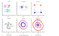
Results of spectral clustering. The figure is taken from here
-
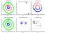
Results of spectral clustering. The figure is taken from here


The most notable issue with spectral clustering is its dependency on the definition of "similar" and/or "dissimilar". For example, suppose a class of students were to be cut into two groups. If weights were given to pairs of students according to the similarity of their gender, then the two groups would presumably be separated into males and females. However, this weighting doesn't account for other similarities the class might have such as colour of clothing worn that day, or less visible similarities such as number of hours slept the previous night. The definition of "similar" is therefore what drove the cut, and not the actual similarities between the students. Spectral clustering is a problem that only has subjective solutions due to the subjective nature of the problem.
Multiclass Spectral Clustering
Spectral clustering can be used in multiclass case by choosing the smallest [math]\displaystyle{ k+1 }[/math] eigenvectors and ignoring the smallest one (associated with [math]\displaystyle{ 0 }[/math] eigenvalue), this will result in a matrix of size [math]\displaystyle{ n * k }[/math] which can be used as a covariate of other clustering algorithm.
Alternatively, the k eigenvectors can be used to create [math]\displaystyle{ 2^k }[/math] clusters where the the cluster to which a point is assigned is given by converting the signs of each element in the matrix to binary then reading off the cluster number of each row as the number whose binary representation is given by that row. This is akin to cutting the data into two parts [math]\displaystyle{ k }[/math] times where each subsequent cut approximates the best ratiocut based cut when the previous cuts have already been made. This assigns points with the same sign in the matrix to the same cluster.
Laplacian Eigenmap
Laplacian eigenmap [13] solves the problem of dimensionality reduction by obtaining the eigenvectors that correspond to the lowest [math]\displaystyle{ {d+1} }[/math] eigenvalues and project the data to these eigenvectors. This is very similar to the spectral clustering.
We can interpret the multiclass spectral clustering as a dimensionality reduction step before applying a clustering technique.
Also spectral clustering can be interpreted from Random walk point of view as explained here [14]: "Random walk is a stochastic process on a graph which moves randomly from node to node. So spectral clustering tries to find a graph partition such that random walk stays long within a cluster and with seldom moves from one cluster to another."
A side note: The frobenius norm of the covariance matrix can measure the linear correlation between two variables, the larger the norm the larger the correlation. And this is true only for linear correlation as for the nonlinear correlation data should be mapped to Hilbert space first before applying the covariance operator and obtain the Schmidt norm to get a measure of dependence. Supervised PCA uses this concept.
The following is a matlab sample code that shows the norm of a covariance matrix for uncorrelated, linearly correlated, non-linearly correlated random variables.
>> X1 = randn(1, 10000);
>> X2 = randn(1, 10000);  % x1 and x2 are independent
>> X = [X1;X2];
>> cov(X')        % 2 by 2 matrix.
%    Covariance is small since x1 and x2 and independent.  So we look at the norm of covariance.
>> norm(cov(X'))  % small as X1 and X2 are independent.
%    This is a measure of correlation between these two, which is a measure of linear dependence.
>> X2 = 2 * X1;
>> X = [X1;X2];
>> cov(X')
>> norm(cov(X')) % large as X1 and X2 are linearly dependent
>> X2 = sin(X1);
>> X = [X1;X2];
>> cov(X')
>> norm(cov(X')) % not large as the dependency between X1 and X2 is not linear.
LE(Laplacian eigenmap) uses the similar approach with LLE. It is fast but sometimes can not provide an ideal outcome. It's difference with other DR(dimension reduction) methods is that LE maintains an ideal robustness while there are outliers in the dataset, which is a property that other DR methods do not process.
Supervised Principal Component Analysis (Lecture 9: Oct. 15, 2014)
Assignment 1 Solutions
Overall the first assignment was done quite well. The average mark for undergrads was approximately 70% and the average grade for graduates was approximately 75%. This lecture will focus on the details of the first assignment and going over the solutions. The solutions will not be posted online.
- Question 1 was done quite well. Some marks were deducted for unusual scaling of eigenvalues (division by (n-1)). In general it is a good idea to scale the eigenvalues, however, it will usually not affect whether the PCA function works or not. Marks were given simply for having a picture for most of the questions. Note that the explanations for the questions should have some detail, one-word answers are not sufficient.
- Question 2 part(a) had some issues. Some students plotted too many eigenvectors. Also in general, the fewer PCs we keep, the better. When determining how many eigenvectors to keep, look for an "elbow" in the plot for when the variance represented by a given eigenvector drops off.
- Question 3 was very well done, as long as you had some pictures, you would have gotten most of the marks.
- Question 4 had some issues. These are very well-known properties, so you should prove it using the definitions and show more detailed steps.
- Question 5 was marked based on how far a student correctly followed the solution. Take the partial derivatives according to [math]\displaystyle{ \mu }[/math], and according to [math]\displaystyle{ y_i }[/math], set equal to 0 and simplify. Substituting one into the other and further simplifying gives the answer.
- Question 6 part(a) as well as part(c) were done well. Part(b) required showing that all eigenvectors of [math]\displaystyle{ \tilde S }[/math] are also eigenvectors of [math]\displaystyle{ \, S }[/math]
Introduction to Supervised Principal Component Analysis
Motivation: There are several applications in which we would like to reduce the dimensionality of data to be able to deal with it easier, however we would like to keep some desired properties or features of data in low dimensional representation at the same time. In fact, we don't want to reduce the dimensionality blindly.
For example, suppose that we would like to rank undergrad students in CS departments in top universities in Canada according to their grades in different courses. Suppose that there are 2000 students and 20 common courses. Since the data set is large, we want to reduce the dimensionality (number of courses) to 3 dimensions to process faster. If we run a PCA algorithm blindly, the algorithm returns the 3 courses in which students' grades have most variation. Assume there is a course (for example, Data Visualization) that we would like to keep in our top three courses because its grade is important in our evaluation.
Sometimes there is a feature or dimension of the data that we don't want to omit during dimensionality reduction. This is where supervised PCA is used.
Principal component analysis (PCA) may not be the ideal way for processing multiple sets of data at once or data with different classes of characteristics (dataset with different modes of variation), since the principal component which maximizes variation may not preserve these characteristics/classes. As such, maximizing the variance sometimes is not the best way to reduce the dimensionality of the data. As shown in the below figure (taken from here [15]), we can see that projecting the data on the direction of maximum variation will not make the two classes discriminated in the lower dimensions compared to FDA.
Sometimes we will do clustering as a pre-algorithm, or we can incorporate side data and use labels in PCA in order to create a better dimensionality reduction. In these cases, we are more interested in finding subspaces with respect to the labels of the original data instead of those that maximizes the variance.

In dimensionality reduction we might have some "side information" or labels. In low dimension data we want points with the same label to be close to each other. Consider if you have a set of images of faces. The different faces can be divided into glasses/no glasses classes or beards/no beards classes, or I have other information about which people are similar. In low dimensional representation I want these points to be close to each other. KPCA may be able to distinguish some pre-specified features in the picture, while PCA could only give components that have max variance. In dimension reduction, we might have some "side information" or labels.
Problem Statement
Given a set of data [math]\displaystyle{ (X,Y),\; X \in \mathbb{R}^p }[/math] are p-dimensional explanatory variates and [math]\displaystyle{ Y\in \mathbb{R}^l }[/math] l-dimensional response variables, the goal is to estimate a low-dimension subspace S such that S contains as much predictive information about the response variable Y as the original explanatory variable X.
Alternatively, given an i.i.d (independent and identically distributed) sample [math]\displaystyle{ \{(x_1,y_1), (x_2,y_2) \dots (x_N,y_N)\} }[/math], we are looking for an orthogonal projection of X onto [math]\displaystyle{ \,S=U^T X }[/math] such that Y depends mainly on [math]\displaystyle{ \,U^T X }[/math].
Related Work
There are many families of algorithms to solve this problem, some of which are briefly described below.
Classical Fisher's discriminant analysis (FDA)
This algorithm is very famous, however it will not be covered in this class. This[16] or [17] are brief introductions to FDA. A brief overview is also given below.
Introduction
Consider a two-class problem, i.e. [math]\displaystyle{ l }[/math] = 1 in the above formulation. For each class, let [math]\displaystyle{ \,\mu_i }[/math] and [math]\displaystyle{ \,\Sigma_i }[/math] denote the mean and covariance matrix of each class, for [math]\displaystyle{ i }[/math] = 0, 1. Using a generic vector [math]\displaystyle{ \,w }[/math], we transform each data point [math]\displaystyle{ \,x_i }[/math] using [math]\displaystyle{ \,w^Tx_i }[/math]. Thus, the new means and covariances are as below:
[math]\displaystyle{ \mu_i^' = \mathbf{w}^T \mu_i }[/math]
[math]\displaystyle{ \Sigma_i^' = \mathbf{w}^T\mathbf{\Sigma_i}\mathbf{w} }[/math]
We would like to minimize the separation within the individual classes (within-class variance), and maximize the separation of the two classes of data (between-class variance), of the projected data.
Solving the Problem
Let [math]\displaystyle{ \mathbf{S}_W = \mathbf{\Sigma_0} + \mathbf{\Sigma_1} }[/math] be the within-class covariance matrix. Then, minimizing the within-class variance is described by:
[math]\displaystyle{ \min_\mathbf{w} \mathbf{w}^T \mathbf{S}_W \mathbf{w} }[/math]
Similarly, let [math]\displaystyle{ \mathbf{S}_B = (\mu_0 - \mu_1)(\mu_0 - \mu_1)^T }[/math] be the between-class covariance matrix. Then, maximizing the between-class variance is described by:
[math]\displaystyle{ \max_\mathbf{w} \mathbf{w}^T \mathbf{S}_B \mathbf{w} }[/math]
We can combine these two optimization problems to simply solve the following:
[math]\displaystyle{ \max_\mathbf{w} \frac{\mathbf{w}^T \mathbf{S}_B \mathbf{w}}{\mathbf{w}^T \mathbf{S}_W \mathbf{w}} }[/math]
This problem is equivalent to:
[math]\displaystyle{ \max_\mathbf{w} \mathbf{w}^T \mathbf{S}_B \mathbf{w}, \mbox{ subject to: } \mathbf{w}^T \mathbf{S}_W \mathbf{w} = 1 }[/math]
This is a generalized eigenvalue problem, where [math]\displaystyle{ \mathbf{w} }[/math] can be computed as the eigenvector of [math]\displaystyle{ \mathbf{S}_W^{-1} \mathbf{S}_B }[/math] with maximal eigenvalue.
Metric Learning (ML)
The technique attempts to construct a Mahalanobis distance over the input space, which could then be used instead of Euclidean distances. ML methods search for a metric (or equivalently, a linear transformation) under which points in the same class (similar points) are near each other and simultaneously far from points in the other classes. We need to minimize the sum of distances between similar class samples and maximize the sum of distance between different class samples.
Euclidean Distance: [math]\displaystyle{ \,(x_i - x_j)^T(x_i - x_j) }[/math]
Mahalanobis Distance: [math]\displaystyle{ \,(X_i - x_j)^TA(x_i - x_j) }[/math] , where A is a positive, semi-definite matrix
Write [math]\displaystyle{ \, A = UU^T }[/math]
[math]\displaystyle{ \,d_A(x_i, x_j) = (U^Tx_i - U^Tx_j)^T(U^Tx_i - U^Tx_j) }[/math]
Thus, we obtain the mapping
[math]\displaystyle{ x \mapsto U^Tx }[/math]
More information can be found in Metric Learning.
This website introduces several strategies on metric selection Distance Metric Learning
Sufficient Dimension Reduction (SDR)
In sufficient dimension reduction, we attempt to find a linear subspace [math]\displaystyle{ S \subset X }[/math] such that [math]\displaystyle{ P_{Y\mid X}(y\mid X) }[/math] is preserved.
i.e [math]\displaystyle{ P_{Y\mid X}(y\mid X) = P_{Y\mid U^TX}(y\mid U^TX)\; \forall x,y }[/math]
Supervised Principal Components (SPCA)
- This version of Supervised Principal Components is different from the the Supervised Principal Component Analysis that we are going to talk about in this lecture. It is proposed by Bair er. al., and the original paper can be found here[18].
- The idea is to perform PCA only on selected data with a strong estimated correlation to the response variable (Y). This removes some unseen factors that are unrelated to the response variable (Y).
- This method is commonly used in biostatistics, but it's different from the one we are covering this course.
Steps
- Recall that in linear regression the coefficient for feature j is computed as: [math]\displaystyle{ s_j = \dfrac{X_j^T Y}{\sqrt{X^T_jX_j}} }[/math]Note that [math]\displaystyle{ X }[/math] doesn't have to be centered. This is essentially a measure of similarity between feature j (row j) and output Y.
- Replace the data matrix so that it only consists of features for whom the absolute value of the calculated coefficients exceeds some determined threshold [math]\displaystyle{ \theta }[/math].
- Compute the first (few) principal components of the reduced data matrix.
- Use the principal component(s) calculated in step 3 in a regression model or classification algorithm to predict the outcome.
SPCA method focuses on a region of interest from the spatial domain as training set, thus it will be more suitable to extract the property of data that is at most interest.
Hilbert-Schmidt Independence Criterion (HSIC)
Two random variables [math]\displaystyle{ X\in \mathbb{R}^p }[/math] and [math]\displaystyle{ Y\in \mathbb{R}^q }[/math] are independent if and only if any bounded continuous function of them is uncorrelated.
If we map these random variables to reproduce kernel Hilbert spaces (RFHS), we can test for correlation. Problem: Given [math]\displaystyle{ {(x_1, y_1), . . . ,(x_m, y_m)}\∼ . Pr(x, y) }[/math] determines whether [math]\displaystyle{ \,Pr(x, y) = Pr(x)Pr(y) }[/math].
To do so, we define a RKHS [math]\displaystyle{ F:X\to \mathbb{R} }[/math] containing all continuous bounded real-valued functions of x,
and a RKHS [math]\displaystyle{ G:Y\to \mathbb{R} }[/math] containing all continuous bounded real-valued functions of y.
Distance correlation can provide a new approach to testing the joint independence of random vectors. Measuring and testing dependence by correlation of distances is explored here.
Let [math]\displaystyle{ Z:= \{(x_1,y_1),\dots, (x_n,y_n) \} \subseteq X\times Y }[/math] be n independent observations from [math]\displaystyle{ \, \rho_{X,Y} }[/math].
An estimator of HSIC is:
- where [math]\displaystyle{ H,K,B \in \mathbb{R}^{n\times n} }[/math], [math]\displaystyle{ \,K_{ij} = K(x_i,x_j) }[/math] is a kernel of X, [math]\displaystyle{ \,B_{ij} = b(y_i,y_j) }[/math] is a kernel of Y,and [math]\displaystyle{ \,H = I - \frac{1}{n}ee^T }[/math] is the centering matrix. Note that K and B are positive semidefinite.
The HSIC is 0 if and only if X and Y are independent. Thus the estimator described above can be used to test for independence. For more details, see [19].
How far are two distributions from each other? A measure of similarity of [math]\displaystyle{ \, P }[/math] and [math]\displaystyle{ \, Q }[/math] is [math]\displaystyle{ \, X \sim P, Y \sim Q }[/math] where P and Q are probability distributions. We can calculate the distance between distributions [math]\displaystyle{ \, P }[/math] and [math]\displaystyle{ \, Q }[/math] as follows:
- [math]\displaystyle{ \mid P-Q \mid^2 = \mid \frac{1}{n}\sum \phi(x_i)-\frac{1}{m}\sum\phi (y_i) \mid^2 }[/math]
- [math]\displaystyle{ = (\frac{1}{n}\sum \phi(x_i)-\frac{1}{m}\sum\phi (y_i))^T (\frac{1}{n}\sum \phi(x_i)-\frac{1}{m}\sum\phi (y_i)) }[/math]
- [math]\displaystyle{ = \frac{1}{n^2} \sum K(x_i,x_j)+\frac{1}{m^2}\sum K(y_i,y_j) -\frac{2}{mn} \sum K(x_i,y_j) }[/math]
So does the mean capture all the characteristics of the distribution in the higher dimensional space. The idea of this measure of distance is counter-intuitive at first glance, since it states that after mapping into high dimension space using [math]\displaystyle{ \phi(x) }[/math], we can measure the distance of distribution by using the mean of the sample data points. It's difficult to find an explicit [math]\displaystyle{ \phi(x) }[/math], but we can use kernel trick to solve the problem.
Note that, the mean in the original dimensions is not enough to capture the characteristics of the distribution. For example, the following figure shows a two different distributions with exact same mean but with different variance. So, say we have a point in 2 dimensions, the first dimension of the point is the mean and the second dimension of the point is the variance. So, this point captures these two characteristic of the distribution. So, in infinity dimension, a point can capture all momentum of the distribution and therefore, only mean in higher space can capture the characteristic of the distribution.

Now that we have a way to measure the distance between two distributions, we have a way to test for independence since:
[math]\displaystyle{ X, Y }[/math] independent [math]\displaystyle{ \Rightarrow P_{X,Y}(x,y) = P_X(x)P_Y(y) \Rightarrow \mid P_{X,Y}(x,y)-P_X(x)P_Y(y) \mid = 0 }[/math]
Hilbert Schmidt Independence Criterion (Lecture 10: Oct. 20, 2014)
Introduction to the Hilbert Schmidt Independence Criterion (HSIC)
Last lecture we reviewed the background and set-up for SPCA. Given data, X, and corresponding labels, Y, if we want to maximize the dependency between [math]\displaystyle{ U^TX }[/math] (the projected data) and [math]\displaystyle{ Y }[/math], then we will need the Hilberts Schmidt Independence Criterion (HSIC). When data are mapped to a higher dimension space (e.g. a kernel), we hope that the data and dependency are both linear with respect to that space. However, some cases won't necessarily conform to these assumptions. This was explained last lecture with the example of two distributions with the same mean, but with different variances.
Intuition: Two random variables [math]\displaystyle{ x }[/math] ~ [math]\displaystyle{ p }[/math] and [math]\displaystyle{ y }[/math] ~ [math]\displaystyle{ q }[/math] in [math]\displaystyle{ R^n }[/math] are independent if and only if any bounded continuous function of them is uncorrelated
[math]\displaystyle{ |p-q|^2 }[/math] (which is called Maximum Mean Discrepancy (MMD) [20]) measures distance between two distributions [math]\displaystyle{ p }[/math] and [math]\displaystyle{ q }[/math]. It also allows us to check independence since [math]\displaystyle{ p(x,y)=p(x)p(y) }[/math] implies independency. We can re-write the distance equation as [math]\displaystyle{ |p(x,y)-p(x)p(y)|^2 }[/math] where expanding [math]\displaystyle{ p(x,y)-p(x)p(y) }[/math] gives the Hilbert Schmidt Independence Criterion (HSIC). This term is based on the norm of the covariance matrix in Hilbert space.
Derivation of HSIC
Goal: Given an [math]\displaystyle{ i.i.d }[/math]. sample, [math]\displaystyle{ \,X }[/math], and labels, [math]\displaystyle{ \,Y }[/math], we want an orthogonal projection of the data onto [math]\displaystyle{ \, U^TX }[/math] such that [math]\displaystyle{ \,Y }[/math] depends on [math]\displaystyle{ \,U^TX }[/math].
An estimator of [math]\displaystyle{ HSIC }[/math] is given by:
- where
- [math]\displaystyle{ K }[/math] is a kernel over [math]\displaystyle{ X }[/math], positive semidefinite
- [math]\displaystyle{ B }[/math] is a kernel over [math]\displaystyle{ Y }[/math], positive semidefinite
- [math]\displaystyle{ H }[/math] is the centering matrix given by [math]\displaystyle{ H=I-\frac{1}{n} ee^T }[/math]
We then want to maximize maximize the dependency of [math]\displaystyle{ \,Y }[/math] on [math]\displaystyle{ \, U^TX }[/math]
This is done by:
- Compute the linear kernel of [math]\displaystyle{ \,U^TX }[/math] :
[math]\displaystyle{ \,K_{n \times n}=X^TUU^TX }[/math] is a [math]\displaystyle{ \,n \times n }[/math] matrix
Notice the similarity to Kernel PCA, which finds [math]\displaystyle{ \,X^TX }[/math], the linear kernel of [math]\displaystyle{ \,X }[/math] - Compute a kernel of labels [math]\displaystyle{ \,Y }[/math] :
[math]\displaystyle{ \,B_{n \times n}=Y^TY }[/math] is a [math]\displaystyle{ \,n \times n }[/math] matrix - According to HSIC, the dependency between [math]\displaystyle{ \,U^TX }[/math] and [math]\displaystyle{ \,Y }[/math] can be computed as
- where [math]\displaystyle{ K_{n \times n}= (U^TX)^T U^T X = X^TUU^TX }[/math]
- Since [math]\displaystyle{ \frac{1}{(n-1)^2} }[/math] doesn't depend on [math]\displaystyle{ U }[/math], we only need to maximize the trace, where the only unknown is [math]\displaystyle{ U }[/math]
- So we solve
- [math]\displaystyle{ \underset{U}{max} \; Tr(X^TUU^TXHBH) }[/math]
- where [math]\displaystyle{ K_{n \times n}= (U^TX)^T U^T X = X^TUU^TX }[/math]
Since the trace of a matrix is invariant under cyclic permutations, this can be rewritten as:
- [math]\displaystyle{ = \underset{U}{max} \; Tr(HX^TUU^TXHB) }[/math]
- [math]\displaystyle{ = ... = \underset{U}{max}\; Tr(U^TXHBHX^TU) }[/math]
- Letting [math]\displaystyle{ \,Q = XHBHX^T }[/math], the problem becomes [math]\displaystyle{ \underset{U}{max} \; Tr(U^TQU) }[/math].
- There is no upper bound on this optimization problem, which means that increasing the elements of U infinitely will increase the objective function infinitely. So, our problem is ill-defined. Thus, we need put such a constraint to restrict [math]\displaystyle{ \,U }[/math] and solve our optimization problem under that consideration.
- Therefore, we are going to solve our objective function such that: [math]\displaystyle{ \,U^TU = I }[/math] (i.e. [math]\displaystyle{ \,U }[/math] is an orthogonal matrix) as our restriction, just like with [math]\displaystyle{ PCA }[/math].
- To solve this problem, use the Lagrange Multipliers:
- The Lagrangian is given by: [math]\displaystyle{ L(U, \Lambda) = Tr(U_{}^TXHBHX^TU^T)-Tr(\Lambda(U^TU-I)) }[/math]
- [math]\displaystyle{ \, = Tr(U^TQU)-Tr(\Lambda(U^TU-I)) }[/math]
- Taking the derivative of this with respect to U and setting to zero yields
- [math]\displaystyle{ \,2QU - 2\Lambda U = 0 }[/math]
- [math]\displaystyle{ \,QU = \Lambda U }[/math]
- [math]\displaystyle{ \,(XHBHX^T)U = \Lambda U }[/math]
- Hence, adding this restriction implies we need to find the [math]\displaystyle{ p }[/math] eigenvectors corresponding to the largest eigenvalues of [math]\displaystyle{ XHBHX^T }[/math] as the columns of [math]\displaystyle{ U }[/math].
- Letting [math]\displaystyle{ \,Q = XHBHX^T }[/math], the problem becomes [math]\displaystyle{ \underset{U}{max} \; Tr(U^TQU) }[/math].
- [math]\displaystyle{ \,U^TX }[/math] is the projection of X on a lower dimension space, but in this context we are ensuring it has maximum dependence on [math]\displaystyle{ Y }[/math], rather than trying to maximize captured variance as with [math]\displaystyle{ PCA }[/math].
Note that if [math]\displaystyle{ \,B=I }[/math], then [math]\displaystyle{ \,X_{}HBHX^T = XHHX^T }[/math]. Since this is now the sample covariance matrix of centered [math]\displaystyle{ \,X }[/math], the solution to [math]\displaystyle{ SPCA }[/math] will be identical to the solution to [math]\displaystyle{ PCA }[/math]. Therefore [math]\displaystyle{ PCA }[/math] is just [math]\displaystyle{ SPCA }[/math] with the condition that [math]\displaystyle{ \,B=I }[/math].
- If [math]\displaystyle{ \,B=I }[/math], then, since [math]\displaystyle{ \,B }[/math] is the kernel over all the labels and so represents the pairwise similarity over labels, we are working only under the knowledge that each datum is similar to itself - we do not know how similar any datum is to another datum. Or we can interpret it as knowing that each sample is in a separate class; this is how PCA is conducted.
- SPCA is therefore PCA with additional knowledge regarding similarity between data. So if you don't have labels use PCA, but if you do have more information about the similarity of the points, then you can impose it using SPCA. Therefore, PCA can be seen as a special case of SPCA.
Algorithm for SPCA
- Recover basis
Calculate [math]\displaystyle{ \; Q=XHBHX^T }[/math]
Define [math]\displaystyle{ U }[/math] based on the top [math]\displaystyle{ p }[/math] eigenvectors of [math]\displaystyle{ Q }[/math] corresponding to the top p eigenvalues - Encode training data
Let [math]\displaystyle{ \; Z=U^TXH }[/math] where [math]\displaystyle{ Z_{d \times n} }[/math] is a [math]\displaystyle{ d \times n }[/math] matrix - Reconstruct training data
[math]\displaystyle{ \hat{X} = UZ = UU^TX }[/math] - Encode test example
[math]\displaystyle{ \; z = U^T*(x-\mu) }[/math] where [math]\displaystyle{ z }[/math] is a [math]\displaystyle{ p }[/math]-dimensional encoding of [math]\displaystyle{ x }[/math] - Reconstruct test example
[math]\displaystyle{ x=Uz = UU^T(x-\mu) \; }[/math]
Note that if [math]\displaystyle{ B }[/math] is the linear kernel over Y then the dimension of the embedding one can create with this algorithm is bounded above by the rank of [math]\displaystyle{ Y^T Y }[/math] since in this case the rank of [math]\displaystyle{ Q }[/math] is bounded above by rank of [math]\displaystyle{ Y^T Y }[/math]. Any additional eigenvectors returned if the algorithm were asked for more would be arbitrary vectors from the null space of [math]\displaystyle{ Q }[/math].
Dual Supervised Principal Component Analysis
Recall how Dual PCA led to Kernel PCA. Dual PCA was based on cases where dimensionality [math]\displaystyle{ d }[/math] of data is large compared to the number of samples [math]\displaystyle{ n }[/math], and hence the eigenvectors of [math]\displaystyle{ \, XX^T_{d*d} }[/math] are hard to find. Instead, singular value decomposition was used to decompose the data into [math]\displaystyle{ X = U \Sigma V^T }[/math] where
- U is the eigenvectors of [math]\displaystyle{ \, XX^T_{d*d} }[/math]
- V is the eigenvectors of [math]\displaystyle{ \ X^TX_{n*n} }[/math]
re-arranging shows [math]\displaystyle{ \ U = XV \Sigma^{-1} }[/math]
Similarly, we can decompose [math]\displaystyle{ \, Q = XHBHX^T }[/math] instead of just decomposing [math]\displaystyle{ X }[/math]. First as [math]\displaystyle{ \Psi }[/math] and [math]\displaystyle{ Q }[/math] are positive semi-definite matrices we define
- [math]\displaystyle{ \ Q = \Psi \Psi^T }[/math] (As it's Positive Semi-Definite (PSD) matrix
- [math]\displaystyle{ \ B = \Delta^T \Delta }[/math]
So [math]\displaystyle{ \ Q = \Psi \Psi^T = XH\Delta^T \Delta H X^T = (XH\Delta^T) (XH^T\Delta^T)^T = (XH\Delta^T) (XH\Delta^T)^T }[/math] So [math]\displaystyle{ \ \Psi }[/math] can be calculated as
- [math]\displaystyle{ \ \Psi =XH \Delta^T }[/math]
The solution for U can be decomposed from [math]\displaystyle{ \, \Psi =U \Sigma V^T }[/math]. Note that DSPCA depends only on the number of points, and is independent of the dimensionality.
Note that if [math]\displaystyle{ B }[/math] is the linear kernel over Y then the dimension of the embedding one can create with this algorithm is bounded above by the rank of [math]\displaystyle{ Y^T Y }[/math] since in this case the rank of [math]\displaystyle{ Q }[/math] is bounded above by rank of [math]\displaystyle{ Y^T Y }[/math]. Any additional eigenvectors returned if the algorithm were asked for more would be arbitrary vectors from the null space of [math]\displaystyle{ Q }[/math].
Kernel Supervised Principal Component Analysis (Kernel SPCA)
In Kernel SPCA, we maximize [math]\displaystyle{ Tr(U^TXHBHX^TU) }[/math] subject to [math]\displaystyle{ U^TU=I }[/math]. There is a trick to doing this: U can be written as a linear combination of all data.
- [math]\displaystyle{ U = \underset{i}{\sum} \alpha_{i} \; x_i }[/math]
This algorithm allows us to re-write our problem using dot product. In matrix form, we assume that, for each column of U, there are n coefficients such that [math]\displaystyle{ \, U=X \beta }[/math] where [math]\displaystyle{ U }[/math] is d x p, [math]\displaystyle{ X }[/math] is d x n, [math]\displaystyle{ \beta }[/math] is n x p
- Our objective function can be re-written in terms of [math]\displaystyle{ \beta }[/math] as
- [math]\displaystyle{ \underset{\beta}{max} \; Tr(U^{T}XHBHX^{T}U) }[/math]
- [math]\displaystyle{ = \underset{\beta}{max} \; Tr(\beta^TX^TXHBHX^TX\beta) }[/math]
- [math]\displaystyle{ = \underset{\beta}{max} \; Tr(\beta^TKHBHK\beta) }[/math]
- notice that [math]\displaystyle{ X^TX }[/math] and [math]\displaystyle{ XX^T }[/math] are our linear kernel: [math]\displaystyle{ \psi (x^T) \psi (x) = \psi (x) \psi (x^T) }[/math]
This constraint term can be re-written in terms of [math]\displaystyle{ \beta }[/math] as:
- [math]\displaystyle{ U^TU=I }[/math] which implies [math]\displaystyle{ \beta^TX^TX \beta = I }[/math] which implies [math]\displaystyle{ \beta^T K \beta = I }[/math]
Therefore the new optimization problem is [math]\displaystyle{ \underset{\beta}{max} \; Tr( \beta^TKHBHK \beta) }[/math] subject to [math]\displaystyle{ \beta^T K \beta = I }[/math]
- Here we don't have [math]\displaystyle{ X }[/math], but rather we have [math]\displaystyle{ K }[/math]. If we were to write the Lagrange multiplier, we can see that the solution to this problem is the generalized eigenvectors of [math]\displaystyle{ HBHK }[/math]:
- [math]\displaystyle{ \; L(\beta) = Tr( \beta^T KHBHK \beta ) - \lambda Tr( \beta^TK \beta - I) }[/math]
- [math]\displaystyle{ \frac{\partial L}{\partial \beta} = 2KHBHK \beta - 2 \lambda K \beta = 0 }[/math]
- [math]\displaystyle{ let \; Q=KHBHK }[/math]
- this implies that [math]\displaystyle{ Q \beta = \lambda K \beta }[/math]
- Notice that if this was just [math]\displaystyle{ Q \beta = \lambda \beta }[/math], then Q would be the eigenvectors, and [math]\displaystyle{ \lambda }[/math] the eigenvalues of [math]\displaystyle{ \beta }[/math]. However, since we instead have [math]\displaystyle{ \lambda K }[/math], we are solving for the generalized eigenvectors of [math]\displaystyle{ \, Q=HBHK }[/math]
- Therefore the solution will be the top p eigenvectors of the generalized eigenproblem [math]\displaystyle{ eigen(Q,K) }[/math]
In high dimensional space, X isn't explicitly available. However, by denoting[math]\displaystyle{ \, X \mapsto\Phi(X) }[/math], then [math]\displaystyle{ \, U= \Phi(X) \Beta }[/math], but we don't have X. Therefore we need to project [math]\displaystyle{ \, \Phi(X) }[/math] to a lower dimension space and compute
[math]\displaystyle{ \, Y=U^T \Phi(X) = \beta^T \Phi^T(X) \Phi(X) = \beta^T K }[/math] where [math]\displaystyle{ \, Y }[/math] is p x n, [math]\displaystyle{ \, \beta^T }[/math] is p x n, and [math]\displaystyle{ \, K }[/math] is n x n.
To project an out-of-sample point, x, we have:
- [math]\displaystyle{ \, y=U^T \Phi(x) = \beta^T \Phi(X) \Phi(x) = \beta^T K_{test} }[/math] where
- [math]\displaystyle{ \, X }[/math] is the training data
- [math]\displaystyle{ \, x }[/math] is the test data
- [math]\displaystyle{ \, K_{test} }[/math] is the kernel between the training and test data. (ie. it codes how similar the training and test data are)
Note: There is an alternative way to derive the Kernel SPCA, which will be shown on Assignment 2
Algorithm for Kernel SPCA
Input:
- [math]\displaystyle{ \mathbf{K} }[/math] the kernel matrix of the training data
- [math]\displaystyle{ \mathbf{K_{test}} }[/math] the kernel matrix of the test data
- [math]\displaystyle{ \mathbf{B} }[/math] kernel matrix of target variable
Note: in lecture note professor use [math]\displaystyle{ \mathbf{L} }[/math] to represent the kernel of target variable. For consistency [math]\displaystyle{ \mathbf{B} }[/math] is used instead.
- [math]\displaystyle{ \mathbf{x} }[/math] testing example
- [math]\displaystyle{ \mathbf{n} }[/math] training data size
Output:
- [math]\displaystyle{ \mathbf{Z} }[/math] dimension reduced training data
- [math]\displaystyle{ \mathbf{z} }[/math] dimension reduced test data
- Define: [math]\displaystyle{ H = I - \frac{1}{n}ee^T }[/math] and [math]\displaystyle{ \ Q = KHBHK }[/math]
- Compute basis: [math]\displaystyle{ \beta_{n \times p} }[/math], the top [math]\displaystyle{ p }[/math] generalized eigenvectors of [math]\displaystyle{ Q }[/math] and [math]\displaystyle{ K }[/math]
- Encode the training data: [math]\displaystyle{ \ Z = \beta^T \Phi^T(X) \Phi(X) = \beta^TK }[/math]
- Encode the test example: [math]\displaystyle{ \ z = \beta^T \Phi^T(X) \Phi(x) = \beta^TK_{test} }[/math]
Note that if [math]\displaystyle{ B }[/math] is the linear kernel over Y then the dimension of the embedding created with this algorithm has an upper bound defined by the rank of [math]\displaystyle{ Y^T Y }[/math]. This is because the rank of [math]\displaystyle{ Q }[/math] is bounded above by rank of [math]\displaystyle{ Y^T Y }[/math]. Any additional eigenvectors returned by the algorithm would be arbitrary vectors generated from the null space of [math]\displaystyle{ Q }[/math].
MATLAB Example for Kernel Matrix
Polynomial degree 4 kernel with kernel function as defined in 'kernel.m'
 >> load X % data to find kernel matrix of
 >>
 >> n = size(X,2);
 >> K = zeros(n);
 >> for i=1:n
 >>      for j =1:n
 >>           K(i,j) = kernel(poly,X(:,i),X(:,j),4,[]);
 >>      end
 >> end
Recommended Kernels for Classification
Delta Kernel
When applying KPCA for classification purposes, the recommended kernel to use on Y is the delta kernel.
[math]\displaystyle{ \mathbf{K}(x, x') = 1 }[/math] if [math]\displaystyle{ \mathbf{x} }[/math] and [math]\displaystyle{ \mathbf{x'} }[/math] are equal, and 0 otherwise.
This kernel distinguishes between elements belonging to different classes.
RBF Kernel
A good kernel to use on X is the Radial Basis Function Kernel (RBF).
[math]\displaystyle{ \mathbf{K}(x, x') = exp(-\frac{\|x-x'\|^2}{2\sigma^2}) }[/math], where [math]\displaystyle{ \mathbf{\sigma} }[/math] is a free parameter.
[math]\displaystyle{ \|x-x'\|^2 }[/math] is the squared Euclidean distance between the two vectors. The value of the RBF kernel decreases as distance between the two vectors increases.
Since the value of the kernel ranges between 0 and 1, it can also be interpreted as a similarity measure.
Experimental Results Visualization
The following images are the 2-dimensional projections to the Iris flower data set produced by (in order from left to right):
a. Supervised PCA with [math]\displaystyle{ L = I }[/math]
b. Bair's SPC
c. Kernel Dimension Reduction
d. Kernel Supervised PCA
The following are two more examples to show the effects of the 4 projections on different data sets. We are going to use the Binary XOR dataset and the Concentric Ring dataset to demonstrate.
The Binary XOR dataset
Original form of the Binary XOR dataset
An 1-dimensional Gaussian noise is added to the dataset before projected to 2-dimensional space.
2-dimensional projections of the Binary XOR dataset produced by (in order from left to right):
a. Supervised PCA with [math]\displaystyle{ L = I }[/math]
b. Bair's SPC
c. Kernel Dimension Reduction
d. Kernel Supervised PCA
KSPCA is able to clearly seperate the data into the 2 categories while the other methods fail to do so
The Concentric Ring dataset
Original form of the Concentric Ring data set

2-dimensional projections of the Concentric Ring dataset produced by (in order from left to right):
a. Supervised PCA with [math]\displaystyle{ L = I }[/math]
b. Bair's SPC
c. Kernel Dimension Reduction
d. Kernel Supervised PCA

KSPCA is able to seperate the data into 2 distinct clusters while the other methods are unble to do so
SPCA continued and Metric Learning(Lecture 12: Oct. 22, 2014)
SPCA continued
SPCA compared to other methods
The following figure compares the performance of different dimensionality reduction techniques across 5 datasets. The one-nearest-neighbor classifier is used, as it doesn't have parameters to tune for each dimensionality reduction algorithm, which guarantees a fair comparison between the different algorithms. (Figure from Supervised principal component analysis: Visualization, classification and regression on subspaces and submanifolds by Barshana, Ghodsi, Azimifara, and Zolghadri Jahromia.)
We can only project up to k-1 dimensions using FDA, where k is the number of classes. Increasing the number of dimensions beyond [math]\displaystyle{ K-1 }[/math] has no effect and the error becomes flat.

Methods like KDR([21]) do not work in all of the datasets above, however SKPCA did pretty well for most of them. The consistently good performance of SKPCA lets us use it as a pre-processing step for any supervised machine learning task, avoiding the curse of dimensionality.
KSPCA has the same runtime efficiency as SPCA because its optimization is based on the number of observations, rather than the dimensionality of the data.
Feature Selection
There are two main approaches for dimensionality reduction [22] [23]
- Feature selection: Selecting a subset of the existing features
- Feature extraction: Combining the existing features to produce a smaller number of features.
The formulation of SPCA can also be used for feature selection as follows:
Remember that we have [math]\displaystyle{ \,U^T X }[/math] as our projection. We computed [math]\displaystyle{ \,U }[/math] in a way that [math]\displaystyle{ \,U^T X }[/math] has maximum dependence with the label [math]\displaystyle{ \,Y }[/math].
Now consider only the first column of [math]\displaystyle{ \,U }[/math] , denote it as the vector [math]\displaystyle{ \,u }[/math]. We can project the data into one dimensional space using this vector [math]\displaystyle{ \,u }[/math].
If vector [math]\displaystyle{ \,u }[/math] is sparse. i.e. [math]\displaystyle{ \,u=[0,0,...0,a,0,...0,b,0,...] }[/math] we multiply it with [math]\displaystyle{ \,X }[/math] to get a linear combination of rows of [math]\displaystyle{ \,X }[/math]. However, since we have a lot of zeros in [math]\displaystyle{ \,u }[/math] the resulting matrix will only contain information of rows that is not multiplied by [math]\displaystyle{ 0 }[/math]. If we remove the unused rows we will still have maximum dependence with the label [math]\displaystyle{ \,Y }[/math]. This is equivalent to saying that we don't need these features/variables, because they have no dependence with [math]\displaystyle{ \,Y }[/math]. (i.e for [math]\displaystyle{ \,u=[0,0,...0,a,0,...0,b,0,...] }[/math], the first few features of Y which corresponds to the first few zero entries of [math]\displaystyle{ \,u }[/math] are redundant.)
To compute sparse eigenvectors, [math]\displaystyle{ \,U }[/math], we can use LASSO [24]. The method was previously interpreted using linear programming in 1999. In 2009, a new efficient algorithm called coordinate descent [25] was introduced.
Using this method we can project the data on only one dimension. If we want to project on [math]\displaystyle{ p }[/math] dimensions we will need to use a [math]\displaystyle{ p }[/math]-column matrix with block-sparsity property. Block sparsity can be achieved by minimizing the [math]\displaystyle{ l_{2,1} }[/math] norm, defined by
Metric Learning
Introduction
Metric learning computes the Mahalanobis distance instead of Euclidean distance over the input space. The Mahalanobis distance is defined as
where [math]\displaystyle{ A }[/math] is a symmetric positive semi-definite matrix.
Motivation and Explanation:
Metric Learning was proposed by Xing et al in 2002. They proposed to construct a new distance metric over the points to use in place of Euclidean distances. In this approach, some amount of side information is employed to learn a distance metric that captures the desired information.
Suppose we only have class-related side information (not as strong as a label) about some data set. For example, we only know a pair of [math]\displaystyle{ \,(x_i, x_j) }[/math] is similar or dissimilar. We notate Set [math]\displaystyle{ \,S }[/math] containing all similar point pairs and Set [math]\displaystyle{ \,D }[/math] containing all dissimilar point pairs:
[math]\displaystyle{ \mathcal{S}: (\boldsymbol{x_i, x_j}) \in \mathcal{S} }[/math] , if [math]\displaystyle{ \boldsymbol{x_i} }[/math] and [math]\displaystyle{ \boldsymbol{x_j} }[/math] are similar;
[math]\displaystyle{ \mathcal{D}: (\boldsymbol{x_i, x_j}) \in \mathcal{D} }[/math] , if [math]\displaystyle{ \boldsymbol{x_i} }[/math] and [math]\displaystyle{ \boldsymbol{x_j} }[/math] are dissimilar.
For square of Euclidean distance between [math]\displaystyle{ \,(x_i, x_j) }[/math],
- [math]\displaystyle{ \, |x_i - x_j|^2 = (x_i - x_j)^T (x_i - x_j) }[/math]
we can generalize it by adding a matrix [math]\displaystyle{ A }[/math]
- [math]\displaystyle{ \, d^2_A(x_i,x_j) = \|x_i - x_j\|_A^2 = (x_i - x_j)^T A (x_i - x_j) }[/math].
Matrix [math]\displaystyle{ A }[/math] should make [math]\displaystyle{ \, d_{ij} }[/math] satisfy the four properties of a metric:
- Non-negativity: [math]\displaystyle{ \,d_{ij} \geq 0 }[/math]
- Coincidence: [math]\displaystyle{ \,d_{ii} = 0 }[/math]
- Symmetry: [math]\displaystyle{ \,d_{ij} = d_{ji} }[/math]
- Triangular Inequality: [math]\displaystyle{ \,d_{ij} +d_{jk} \geq d_{ik} }[/math]
It can be proven that when Matrix [math]\displaystyle{ A }[/math] is positive semi-definite, [math]\displaystyle{ \, d_{ij} }[/math] must satisfy these four properties. The distance [math]\displaystyle{ \, d_{ij} }[/math] is called the Mahalanobis distance.
Note that Mahalanobis distance is equivalent to Euclidean distance by doing Cholesky decomposition to Matrix [math]\displaystyle{ A }[/math].
thus, we have
[math]\displaystyle{ \, d^2_A(x_i,x_j) = (x_i - x_j)^T A (x_i - x_j) }[/math]
[math]\displaystyle{ \, = (x_i - x_j)^T w w^T (x_i - x_j) }[/math]
[math]\displaystyle{ \, = (w^T x_i - w^T x_j)^T (w^T x_i - w^T x_j) }[/math]
This can be interpreted as calculating the Euclidean distance after transforming [math]\displaystyle{ X }[/math] using transformation matrix [math]\displaystyle{ W }[/math] by [math]\displaystyle{ f(x)=W^TX }[/math].
Distance Metric Learning
The main idea behind this method is to minimize the sum of distances between samples that should be similar while maximizing the sum of distances between samples that should be dissimilar. We need to find a matrix A that accomplishes this given that Matrix A is positive semidefinite, i.e. [math]\displaystyle{ \, A \geq 0 }[/math].
We can define an Objective Function where we want to minimize the sum of the distances between the pairs of points in Set S:
[math]\displaystyle{ \, min_{A} \sum_{(x_i,x_j) \in S} d_{ij}^2 = min_{A} \sum_{(x_i,x_j) \in S} ||x_i -x_j ||^2_A }[/math]
When [math]\displaystyle{ \, A =0 }[/math], this criterion becomes not useful. We define the following constraint:
[math]\displaystyle{ \, \sum_{(x_i,x_j) \in D} ||x_i -x_j ||_A \geq 1 }[/math]
(Notice, not squared). This constraint is necessary because, if points are dissimilar, we don't want them to collapse into a single point. So we set the criterion to be, arbitrarily, greater or equal to 1.
The matrix [math]\displaystyle{ A }[/math] changes the definition of distance/similarity. But we don't know A, so the problem is then reduced to finding [math]\displaystyle{ A }[/math].
Xing et al proposed an approach to get Matrix A by Newton-Raphson method. However, this approach does not work well.
MCML approach (Maximally Collapsing Metric Learning)
A popular and efficient approach is Maximally Collapsing Metric Learning, proposed by Amir Globerson and Sam Roweis. The objective function here is a set of conditional probabilities [math]\displaystyle{ p^A(j|i) }[/math]. For each [math]\displaystyle{ \, x_i }[/math], the authors introduced a conditional distribution over points [math]\displaystyle{ i \neq j }[/math] such that
[math]\displaystyle{ p^A(j|i) = \dfrac {e^{-d^A_{ij}}}{\sum_{k \neq i} e^{-d^A_{ik}}} ~~ i \neq j }[/math]
In an ideal situation, all points in Set S (similar set) are mapped to a single point and are mapped infinitely far from the points in Set D (dissimilar set). The ideal distribution is then:
[math]\displaystyle{ p_0 (j | i) \propto \begin{cases} 1& y_i=y_j\\ 0& y_i \neq y_j. \end{cases} }[/math]
Our goal is to make the conditional as close as possible to the ideal case. When [math]\displaystyle{ \,p^A(j|i) = p_0 (j | i) }[/math], then under A all points in the same class will be mapped to a single point, infinitely far from other class points. Thus our objective is to find a Matrix A such that [math]\displaystyle{ \,p^A(j|i) }[/math] is as close to [math]\displaystyle{ \, p_0 (j | i) }[/math] as possible. KL divergence [27] is applied to solve it.
KL divergence is a measure of the difference between two probability distributions. We denote the difference between probability distribution [math]\displaystyle{ \,P }[/math] and [math]\displaystyle{ \,Q }[/math] by [math]\displaystyle{ \,D_{KL}[P|Q] }[/math].
Thus, the objective becomes minimizing the KL divergence between [math]\displaystyle{ \,p_0 }[/math] and [math]\displaystyle{ \,p^A }[/math], i.e.
[math]\displaystyle{ min \sum_i KL[p_0(j|i)|p^A(j|i)] ~~ s.t ~~ A \geq 0 }[/math]
Learning a Metric from Class-Equivalence Side Information
Ghodsi et al 's approach
Instead of minimizing the Mahalanobis distance, we define a loss function, which, when minimized, attempts to minimize the squared induced distance between similar points and maximize the squared induced distance between dissimilar points. So the new objective function becomes:
[math]\displaystyle{ L(A) = \dfrac {1}{\left| S\right|} \sum_{(x_i,x_j) \in S} ||x_i -x_j ||^2_A - \dfrac {1}{\left| D\right|} \sum_{(x_i,x_j) \in D} ||x_i -x_j ||^2_A }[/math]
The optimization problem then becomes [math]\displaystyle{ \, min_{A} L(A) }[/math] such that [math]\displaystyle{ \, A\geq 0 }[/math] and [math]\displaystyle{ \, Tr\left( A\right) =1 }[/math].
The Matrix [math]\displaystyle{ \, A }[/math] should still be positive semi-definite, hence the first constraint.
We also don't want to get a trivial solution of [math]\displaystyle{ \, A }[/math] being 0 matrix (i.e. all zero distances), hence the second constraint.
Consider[math]\displaystyle{ \,\sum_{(x_i,x_j) \in S} ||x_i -x_j ||^2_A }[/math], we can rewrite it as [math]\displaystyle{ \,\sum_{(x_i,x_j) \in S} (x_i-x_j)^T A (x_i-x_j) }[/math]
The term inside the summation is a constant, therefore it can be written as
Since [math]\displaystyle{ \,A }[/math]is positive semi-definite, therefore [math]\displaystyle{ \,A = W^T W }[/math]
we can write the equation as
[math]\displaystyle{ \,\,\sum_{(x_i,x_j) \in S} ||x_i -x_j ||^2_A=\sum_{(x_i,x_j) \in S} Tr[(x_i-x_j)^T W^T W (x_i-x_j)] }[/math]
Again, since the term inside the trace is a constant, we can write it as
So the objective function becomes:
[math]\displaystyle{ \, min_{A} \quad L(A) = \dfrac {1}{\left| S\right|} \sum_{(x_i,x_j) \in S} Tr[W^T (x_i-x_j) (x_i-x_j)^T W] \quad - \quad \dfrac {1}{\left| D\right|} \sum_{(x_i,x_j) \in D} Tr[W^T (x_i-x_j) (x_i-x_j)^T W] }[/math]
We can further simply it by letting
[math]\displaystyle{ \, M_S = \dfrac {1}{\left| S\right|} \sum_{(x_i,x_j) \in S} (x_i-x_j) (x_i-x_j)^T }[/math]
[math]\displaystyle{ \, M_D = \dfrac {1}{\left| D\right|} \sum_{(x_i,x_j) \in D} (x_i-x_j) (x_i-x_j)^T }[/math]
and rewriting the equation as
[math]\displaystyle{ \, min_{A} \quad L(A) = Tr[W^T M_S W] - Tr[W^T M_D W] = Tr[W^T (M_S - M_D) W] }[/math]
such that
[math]\displaystyle{ \,Tr(A) =1 }[/math] or [math]\displaystyle{ \,Tr(W W^T) =1 }[/math]
Now we use Lagrange Multiplier:
[math]\displaystyle{ \,Tr(W^T (M_S - M_D) W) - \lambda(Tr(W W^T)-1) = 0 }[/math]
We get:
[math]\displaystyle{ \,(M_S - M_D)W = \lambda W }[/math]
It implies that [math]\displaystyle{ \,W }[/math] are eigenvectors of the matrix [math]\displaystyle{ \,M_S - M_D }[/math]
or the solution is the P smallest eigenvectors of the matrix [math]\displaystyle{ \,M_S - M_D }[/math]
Hence we can find [math]\displaystyle{ \, A=W W^T }[/math] easily.
Advantages over Distance Metric Learning
Aside from its convenient form, this formulation has other advantages over that used by Xing et al., especially with respect to the side information they convey Ghodsi et al
Xing et al. require at least one dissimilar pair in order to avoid a solution where all distances are zero. On the other hand, the constraint employed on the trace in this approach means that no restrictions need to be placed on the pairings. Side information can consist of similar pairs only, dissimilar pairs only, or any combination of the two.
In the absence of specific information regarding dissimilarities, Xing et al. assume that all points not explicitly identified as similar are dissimilar. This may be misleading and may force the algorithm to separate points that are actually similar. The formulation in Ghodsi et al. approach uses only the side information one actually has, partitioning the pairings into similar, dissimilar, and unknown.
Embeddings
Two sets of informed embeddings were generated from the same data set, each with side information pertaining to two different characteristics. The embeddings were generated with and without a preprocessing step. The preprocessing step informs the preprocessed embeddings about the characteristic of interest. It uses the new distances calculated with the learned metric.
In this experiment, all similar pairs were identified but no dissimilar pairs (five-pairs beards and all-pairs glasses omitted). The pairs were selected at random. The "Equivalence-Informed MDS" uses the preprocessor.
Inspection (of this and other Figures) reveals that, in general, the informed versions of the embeddings manage to separate the data based on the target property, whereas the uninformed versions are typically chaotic. Side information can be used to capture characteristics of interest where uninformed embedding techniques fail to automatically discover them. Moreover, two different characteristics (beards and glasses) have been captured within the same data set, even when using only small quantities of class-equivalence side information.
Generally, preprocessing is effective with a wide range of embedding techniques.
Dimensionality issue with this approach
We showed previously that W satisfies
[math]\displaystyle{ \,(M_s - M_D)W = \lambda W }[/math]
So W is composed of eigenvectors of the matrix [math]\displaystyle{ \,M_S-M_D }[/math].
However, all these eigenvectors have to correspond to the same eigenvalue [math]\displaystyle{ \,\lambda }[/math].
This implies that the rank of the matrix [math]\displaystyle{ \,M_S - M_D }[/math] is 1.
So the dimensionality of the reconstructed data is only of dimension 1.
This is due to the constraint [math]\displaystyle{ \,Tr(W W^T) = 1 }[/math] that we picked initially. We can modify this constraint so that the rank of the solution matrix [math]\displaystyle{ \,A }[/math] is greater than 1.
Solution with other constraints
In order to get more eigenvalues, possible new constraints were proposed.
One of them is to let
[math]\displaystyle{ \, W^T W = I }[/math]
We follow similar procedure as the original approach.
Using the Lagrange Multiplier we get:
[math]\displaystyle{ \,Tr(W^T (M_S - M_D) W) - Tr(\Lambda (W^T W - I)) = 0 }[/math]
[math]\displaystyle{ \,(M_S - M_D)W = \Lambda W }[/math], where [math]\displaystyle{ \,\Lambda }[/math] is a diagonal matrix containing the coefficients.
Since we are minimizing the objective function. The solution for [math]\displaystyle{ \,W }[/math] will be p smallest eigenvectors of
Now that we learned that changing our constraint will change our solution, we can think of this constraint more carefully. Another constraint we can have is:
[math]\displaystyle{ \,W^T M_S W = I }[/math]
Basically, rescale each direction by the variance of points in that direction.
Relation to FDA
Recall that FDA solution is the eigenvectors of [math]\displaystyle{ \mathbf{S_w^{-1} * S_B} }[/math] Where
[math]\displaystyle{ \mathbf{S_w = \sum_c\sum_{i \in c}(x_i - \mu_c) * (x_i - \mu_c)^T} }[/math]
[math]\displaystyle{ \mathbf{S_B = \sum_c(\hat{x} - \mu_c) * (\hat{x} - \mu_c)^T} }[/math]
[math]\displaystyle{ \mathbf{S_w} }[/math] is called within class co-variance. [math]\displaystyle{ \mathbf{S_B} }[/math] is called between class co-variance.
Recall MCML solution is the eigenvectors of MS - MD.
Conceptually FDA and MCML are similar as FDA evaluate eigenvectors of within class (similar to S similar objects in MCML) and between class (similar to D different objects in MCML).
Non-negative Matrix Factorization Via Rank-one Downdate(NMF) (Lecture 13: Oct 27, 2014)
The following was finished with reference to Nonnegative matrix factorization via rank-one downdate (Ghodsi et al 2008) [28]. The video of the presentation for this paper can be found at this link [29]
Background
Several problems in information retrieval can be posed as low-rank matrix approximation. The seminal paper by Deerwester et al. (1990) on latent semantic indexing (LSI) [30] showed that approximating a term-document matrix describing a corpus of articles via the SVD led to powerful query and classification techniques. A drawback of LSI is that the low-rank factors in general will have both positive and negative entries, and there is no obvious statistical interpretation of the negative entries.
Non-negative matrix factorization might be useful for image segmentation, such that all the basis images are non-negative. For example, below we see two basis images. The one on left contains only non-negative entries. The one on right does not have this constraint.
-

Example 1: Basis image with only positive entries
-

Example 2: Basis image with both positive and negative entries


We see the photo on the left looks more like a normal face, since faces do not have negative entries.
Another application is text analysis. We can use a term frequency matrix to represent the number of times a word appears in different pieces of text. A non-negative matrix is suitable here because a word cannot appear in a given text a negative number of times. Other possible applications include DNA analysis and retrieving notes from polyphonic music.
History
Nonnegative matrix factorization has its roots in the work of Gregory and Pullman (1983), Paatero and Tapper (1994) and Cohen and Rothblum (1993). However, in the field of chemometrics - the study of using data-driven approaches to extract information from chemical systems - a similar method to NMF has been around for a while as something called "Self Modelling Curve Resolution". The vectors in the matrices are seen as continuous curves, as opposed to discrete vectors. Lee and Seung (1999) proposed nonnegative matrix factorization (NMF) as used commonly today: given a matrix A ∈ Rm×n, we want to find non-negative matrix factors W ∈ Rm×k and H ∈ Rk×n such that [math]\displaystyle{ A\approx WH }[/math], both W and H have nonnegative entries, and k ≤ min(m, n).
In a related work, Hofmann (1999) demonstrated an application of NMF to text retrieval. Suppose the original matrix M represents text data, such that each column represents the counts over words appearing in documents. Then when W and H have been found, the columns of W can be considered topics affecting the entire corpus, while the columns of H are mixing proportions specifying the intensity of each topic in each document.
Since the problem is NP-hard (Vavasis, 2007), it is not surprising that no algorithm is known to solve NMF to optimality. Heuristic algorithms proposed for NMF have generally been based on incrementally improving the objective [math]\displaystyle{ \,\left\|A - WH\right\| }[/math] in some norm using local moves.
Perron-Frobenius Theorem
Perron-Frobenius Theorem
Leading singular vectors of a non-negative matrix are non-negative.
This immediately suggests that there is a trivial rank-one NMF:
Compute [math]\displaystyle{ [U,\, \Sigma,\, V] = svd(A)  }[/math] ;
[math]\displaystyle{  W = U_{:1} \,  }[/math];
[math]\displaystyle{  H = \Sigma_{11}  V_{:1}^T  }[/math];
Therefore, [math]\displaystyle{ W H = U_{:1} \Sigma_{11} V_{:1}^T \approx A }[/math].
However this is a rank one approximation of the matrix [math]\displaystyle{ A }[/math] which is not useful in many cases
Power Method for Singular Value Decomposition
Power method computes the leading singular vectors / values (or eigenvectors / eigenvalues) of a matrix using an iterative approach. First, it chooses a random solution and then iteratively tries to improve the answer until the answer converges.
In the algorithm below, we make a random guess for the vector u (for example, a vector of ones). The algorithm then repeats until u, σ, v converge.
Algorithm for SVD using power method

input A ∈ R m×n and k ≤ min(m, n)
output U, Σ, V
1: for µ = 1 to k do
2:   Select a random nonzero u ∈ Rm
3:   u = u/‖u‖
4:   repeat {power method}
5:     v = ATu/‖ATu‖
6:     σ = ‖Av‖
7:     u = Av/‖Av‖
8:   until stagnation in u, σ, v
9:   A = A − uσvT
10:  U(:, µ) = u
11:  V (:, µ) = v
12:  Σ(µ, µ) = σ
13:end for
Note that there is no guarantee that the entries of the residual matrix A in line 9 are still non-negative, therefore this algorithm cannot be used directly as an NMF algorithm for k ≥ 2.
One intuitive idea is that we can replace all negative entries of the residual matrix A with 0, but this is obviously not a very good method.
First Attempt to NMF
Modify the above algorithm following our intuitive idea, we have the following algorithm for NMF based on power method:
Algorithm for NMF based on power method

input A ∈ R m×n and k ≤ min(m, n)
output W, H
1: for µ = 1 to k do
2: Select a random nonzero u ∈ Rm
3:   u = u/‖u‖
4:   repeat {power method}
5:     v = ATu/‖ATu‖
6:     σ = ‖Av‖
7:     u = Av/‖Av‖
8:   until stagnation in u, σ, v
9:   A = A − uσvT
10:  Replace negative entries of A with 0
11:  U(:, µ) = u
12:  V (:, µ) = v
13:  Σ(µ, µ) = σ
14:end for
15:W = UΣ
16:H = VT
The problem is that when changing the negative entries of the residual matrix [math]\displaystyle{ A-u_1\sigma_1v_1 }[/math] to zero, we cannot assure that the modified matrix is similar to the original residual matrix.
Similarity to Clustering
Given [math]\displaystyle{ [u, σ, v] = powermethod(A) }[/math], our second observation is that singular vectors can be used to cluster rows and columns of A. Namely, similar entries in u correspond to similar rows of A, and similar entries in v correspond to similar columns of A.
For the reasoning behind, we can refer to spectral clustering, or the algorithm of power method, where we have [math]\displaystyle{ u = \frac{Av}{ || Av || } }[/math] and [math]\displaystyle{ v = \frac{A^T u}{ || A^T u || } }[/math] . Note that [math]\displaystyle{ u(i) = A(i, :)v }[/math], entries of u can be view as cosine similarity between rows of A with v. If we cluster u and v and replace the entries in the cluster with smaller mean with 0, then we are reconstructing only part of the matrix A.
Algorithm for Modified Power Iteration

1: Find initial v using power method
2: while not converged
3:   u = Av / ‖Av‖
4:   cluster u and remove the cluster with smaller mean
5:   v = ATu / ‖ATu‖
6:   cluster v and remove the cluster with smaller mean
7:   σ = ‖ATu‖
8: end
Rank-One Downdate (R1D)
Objective: find M, N such that A(M, N) is large and approximately rank-one: [math]\displaystyle{ A(M, N) \approx \boldsymbol{u \sigma v^T} }[/math]. You can find the reference paper of Rank-One Downdate here [31].
Therefore the objective function can be written as:
[math]\displaystyle{ max\, f(M, N, \boldsymbol{u}, \boldsymbol{\sigma}, \boldsymbol{v}) = \| A(M, N) \|_F^2 - \gamma \| A(M, N) - \boldsymbol{u}\boldsymbol{\sigma} \boldsymbol{v}^T \|_F^2 }[/math]
This optimization problem is separable, so for each row i:
[math]\displaystyle{ max\, \| A(i, N) \|_F^2 - \gamma \| A(i, N) - \boldsymbol{u}\boldsymbol{\sigma} \boldsymbol{v}^T \|_F^2 }[/math]
If N and [math]\displaystyle{ \boldsymbol{v} }[/math] are given, then M and [math]\displaystyle{ \boldsymbol{u} }[/math] can be computed via least square method, and vice versa.
In the second term [math]\displaystyle{ \| A(i, N) - \boldsymbol{u}\boldsymbol{\sigma} \boldsymbol{v}^T \|_F^2 }[/math], assume N and [math]\displaystyle{ \boldsymbol{v} }[/math] are known, we have [math]\displaystyle{ \boldsymbol{u\sigma} = A(i, N)\boldsymbol{v} }[/math] by least square method.
[math]\displaystyle{ \| A(i, N) \|_F^2 - \gamma \| A(i, N) - \boldsymbol{u}\boldsymbol{\sigma} \boldsymbol{v}^T \|_F^2 }[/math]
[math]\displaystyle{ = A(i, N)A(i, N)^T - \gamma \left( A(i, N)-A(i, N)\boldsymbol{v}\boldsymbol{v}^T\right) \left( A(i, N)-A(i, N)\boldsymbol{v}\boldsymbol{v}^T\right)^T }[/math]
[math]\displaystyle{ = A(i, N)A(i, N)^T - \gamma \left( A(i, N)A(i, N)^T + A(i, N)\boldsymbol{v}\boldsymbol{v}^T\boldsymbol{v}\boldsymbol{v}^T A(i, N)^T -2A(i, N)\boldsymbol{v}\boldsymbol{v}^TA(i, N)^T \right) }[/math]
[math]\displaystyle{ = A(i, N)A(i, N)^T - \gamma \left( A(i, N)A(i, N)^T - A(i, N)\boldsymbol{v}\boldsymbol{v}^TA(i, N)^T \right) }[/math]
[math]\displaystyle{ = (1 - \gamma)A(i, N)A(i, N)^T + \gamma A(i, N)\boldsymbol{v}\boldsymbol{v}^TA(i, N)^T }[/math]
[math]\displaystyle{ = (1 - \gamma)A(i, N)A(i, N)^T + \gamma \left( A(i, N)\boldsymbol{v} \right)^2 }[/math]
Therefore,
[math]\displaystyle{ f(M, N, \boldsymbol{u}, \boldsymbol{\sigma}, \boldsymbol{v}) = \sum_{i} \gamma \left( A(i, N)\boldsymbol{v} \right)^2 + (1 - \gamma)A(i, N)A(i, N)^T }[/math]
where each item in the summation represents the contribution of a row of A in the objective function. Intuitively, we can go through each row of A, calculate its contribution, and keep those that have positive contribution and drop those that have negative contribution.
Algorithm R1D

input A ∈ Rm×n, k > 0
output W ∈ Rm×k, H ∈ Rn×k
1: for µ = 1 to k do
2:   [M, N, u, v, σ] = ApproxRankOneSubmatrix(A)
3:   W(M, µ) = u(M)
4:   H(N, µ) = σv(N)
5:   A(M, N) = 0
6: end for
The ApproxRankOneSubmatrix procedure could be formulated as follows:
Algorithm ApproxRankOneSubmatrix

input A ∈ Rm×n, parameter γ > 1
output M ⊂ {1,...,m}, N ⊂ {1,...,n},
       u ∈ Rm, v ∈ Rn, σ ∈ R
1: Select j0 ∈ {1, . . . , n} to maximize ‖A(:, j0)‖
2: M = {1,..., m}
3: N = {j0}
4: σ = ‖A(:, j0)‖
5: u = A(:, j0)/σ
6: repeat
7:   Let v = A(M, :)Tu(M)
8:       N = {j: γv(j)2 - ‖A(M, j)‖ > 0}
9:       v(N) = v(N)/‖v(N)‖
10:  Let u = A(:, N)v(N)
11:      M = {i: γu(i)2 - ‖A(i, N)‖ > 0}
12:      σ = ‖u(M)‖
13:      u(M) = u(M)/σ
14:until stagnation in M, N, u, σ, v
The basic idea would be repeatedly select a subset of rows and columns, based on the criteria whether they could contribute (as positive) to the sum of the rows/columns.
The R1D algorithm is quite scalable, as it does not need all the data to be kept in memory at once.
Some Results
The results in this section comes from [32].
In Tables 1 and 2 result of LIS and R1D algorithms are presented on the TDT Pilot Study (TDT Study, 1997). The columns of each table are the leading columns of W, with the leading terms per column displayed.

The LSI results show that the topics are not properly separated and terms from different topics recur or are mixed.

The columns in the R1D table are clearly identifiable topics, and the terms in each columns are all correctly associated with the given topics.
The following figure shows a simple binary image dataset (a), where each of the images is composed of one or two basis "triangles". The leftmost column of (b) and (c) illustrates the four leading columns of W which can be interpreted as the learned features. For each feature the images with the largest entries in the corresponding columns in H is showed to the right of each feature. The below figure shows that R1D can learn the correct basis (triangles as features and assign the suitable image to that base while the results of LSI are can not be interpreted (This may be due to assigning negative weights).
-
![Taken from [3]](/statwiki/images/thumb/3/37/R1D_results_1.PNG/102px-R1D_results_1.PNG)
Taken from [3]
![Taken from [3]](/statwiki/index.php?title=File:R1D_results_1.PNG)
The below figure shows the results of R1D and LSI on Freyface dataset where also figures (b) and (c) illustrates the eigenfaces (leading columns of W) of discovered by R1D and LSI respectively. And the images with max entries in the corresponding columns in H. This figure shows that R1D have interpretable results more than LSI.
-
![Taken from [4]](/statwiki/images/thumb/a/a9/R1D_results_2.PNG/70px-R1D_results_2.PNG)
Taken from [4]
![Taken from [4]](/statwiki/index.php?title=File:R1D_results_2.PNG)
![[1]](http://en.wikipedia.org/wiki/File:Min-cut.svg)
Text/Image Biclustering, Nyström Approximation, and Clustering (Lecture 14: Oct 29, 2014)
Text and Image Biclustering
In this section, we discuss two different methods for clustering of images and text: LSI (Latent Semantic Indexing), and R1D.
LSI (Latent Semantic Indexing)
Latent Semantic Indexing is one method for grouping text or images together. In the case of text, the LSI algorithm takes as input a set of documents as a matrix. The [math]\displaystyle{ \, m }[/math] columns of this matrix can represent [math]\displaystyle{ \, m }[/math] documents, and the [math]\displaystyle{ \, n }[/math] rows of this matrix represent all of the words present in the entire document set. The [math]\displaystyle{ \, ij^{th} }[/math] entry of the input matrix generally represents the number of times that term [math]\displaystyle{ \, i }[/math] appears in document [math]\displaystyle{ \, j }[/math]. It is common to rescale the raw frequencies of the input matrix to combat noisy data.
LSI proceeds to group the data by expressing the input matrix [math]\displaystyle{ \, X }[/math] as [math]\displaystyle{ X \approx W * H^T }[/math].
[math]\displaystyle{ \, W }[/math] is an [math]\displaystyle{ \, n \times p }[/math] matrix, and it can be viewed as a basis for the set of documents. [math]\displaystyle{ \, H }[/math] is an [math]\displaystyle{ \, m \times p }[/math] matrix, and it can be viewed as the expression of the basis elements (i.e. the coefficients for each document expressed in the [math]\displaystyle{ \, W }[/math] basis). [math]\displaystyle{ \, p }[/math] is a parameter, and is taken as an integer that is much smaller than [math]\displaystyle{ \, m }[/math] or [math]\displaystyle{ \, n }[/math].
Determining the [math]\displaystyle{ \, W }[/math] and [math]\displaystyle{ \, H }[/math] matrices is done identically to PCA except that we do not need to assume that the [math]\displaystyle{ \, X }[/math] matrix has zero mean. This is also equivalent to taking a Singular Value Decomposition of the data.
In the case that the [math]\displaystyle{ \, X }[/math] matrix is considered to be text, we interpret the basis to be different topics that are present in the document corpus. We can then cluster documents based on the coefficients used to represent them in this basis. Conversely, we can cluster terms based on their similarity to the basis vectors.
Unfortunately, this type of method does not do the best job of distinguishing topics, as seen in the example used in class.
R1D
R1D is another method for grouping text or images (or other sets of data). R1D is very similar to Non-negative Matrix Factorization, and text clustering for R1D can be formulated similarly to the above.
As seen in the example in class, R1D does a very good job of extracting distinct, important features from a large set of data. In both the image segmentation and text clustering examples, R1D significantly outperformed LSI in interpretation and differentiation of features. R1D is scalable, and can easily be applied to large data sets. The implementation only requires one row or column of the data in memory at any given time.
Nyström Approximation
Many of the algorithms we have seen thus far are not scalable on large data sets. Finding the eigenvalue decomposition of an [math]\displaystyle{ \,n }[/math] by [math]\displaystyle{ \,n }[/math] matrix for large [math]\displaystyle{ \,n }[/math] is very computationally expensive. A solution to this is the Nyström Approximation. The aim of Nyström approximation is that for large scale of data set, we randomly choose a subset of data using the result of singular decomposition of this subset of kernel matrix to approximate the whole singular decomposition of its kernel matrix.
Suppose that we have n data points [math]\displaystyle{ \, x_i }[/math] for [math]\displaystyle{ \, i = 1, 2, ..., n }[/math] and we select [math]\displaystyle{ \,m }[/math] data points randomly ([math]\displaystyle{ \,m\lt n }[/math]).
Without loss of generality, we write this data set in this form:
[math]\displaystyle{ \, X = \begin{bmatrix} x_1, x_2 ,..., x_m, x_{m+1},..., x_n \end{bmatrix} }[/math]
Then, we let [math]\displaystyle{ \, R = \begin{bmatrix} x_1, x_2 ,..., x_m\end{bmatrix} }[/math] and [math]\displaystyle{ \, S = \begin{bmatrix} x_{m+1}, x_{m+2} ,..., x_n\end{bmatrix} }[/math]
The data set can be written as
[math]\displaystyle{ \, X = \begin{bmatrix} R&S\end{bmatrix} }[/math].
Now we'll compute the kernel matrix
[math]\displaystyle{ \, K = X^TX= \begin{bmatrix} R^T\\S^T\end{bmatrix}\begin{bmatrix} R&S\end{bmatrix}=\begin{bmatrix} R^TR&R^TS\\S^TR&S^TS\end{bmatrix} }[/math].
Let [math]\displaystyle{ \,A= R^TR }[/math], [math]\displaystyle{ \,B= R^TS }[/math] and [math]\displaystyle{ \,C= S^TS }[/math] where [math]\displaystyle{ \,A }[/math] is an [math]\displaystyle{ \,m }[/math] x [math]\displaystyle{ \,m }[/math] matrix, [math]\displaystyle{ \,B }[/math] is an [math]\displaystyle{ \,m }[/math] x [math]\displaystyle{ \,(n-m) }[/math] matrix, and [math]\displaystyle{ \,C }[/math] is an [math]\displaystyle{ \,(n-m) }[/math] x [math]\displaystyle{ \,(n-m) }[/math] matrix. Then,
[math]\displaystyle{ \, K =\begin{bmatrix} R^TR&R^TS\\S^TR&S^TS\end{bmatrix}=\begin{bmatrix} A&B\\B^T&C\end{bmatrix}_{n \times n} }[/math].
Now, since [math]\displaystyle{ \, A=R^TR }[/math] is s.p.d (symmetric positive definite), we can apply SVD to matrix [math]\displaystyle{ \, A }[/math]:
[math]\displaystyle{ \, A = U{\Sigma}U^T=U{\Sigma}^\frac{1}{2}{\Sigma}^\frac{1}{2}U^T = R^TR }[/math]
where [math]\displaystyle{ R = {\Sigma}^\frac{1}{2}U^T }[/math].
Therefore, we can use this outcome to calculate [math]\displaystyle{ \, S }[/math]:
[math]\displaystyle{ B = R^TS = U{\Sigma}^\frac{1}{2}S }[/math]
U is orthonormal, so we can multiply both sides by [math]\displaystyle{ \, U^T }[/math] and we get:
[math]\displaystyle{ U^TB = U^TU{\Sigma}^\frac{1}{2}S = {\Sigma}^\frac{1}{2}S }[/math]
[math]\displaystyle{ {\Sigma}^{-\frac{1}{2}}U^TB = S }[/math]
therefore [math]\displaystyle{ C = S^TS = B^TU {\Sigma}^{-\frac{1}{2}} {\Sigma}^{-\frac{1}{2}}U^TB = B^TU{\Sigma}^{-1}U^TB = B^TA^{-1}B }[/math]
Note that [math]\displaystyle{ \, A = U{\Sigma}U^T }[/math] so the inverse matrix is[math]\displaystyle{ \, A^{-1} = U{\Sigma}^{-1}U^T }[/math]
Thus, we have [math]\displaystyle{ K = \begin{bmatrix} A&B\\B^T&B^TA^{-1}B\end{bmatrix} }[/math]
Thus, knowing the first [math]\displaystyle{ \,m }[/math] rows of the Kernel matrix allows us to compute the rest of matrix using this method. Also, the approximation is exact if the rank of the Kernel matrix [math]\displaystyle{ \, K \lt = m }[/math].
Example: Apply Nyström approximation to MDS
Recall that MDS starts with an [math]\displaystyle{ n \times n }[/math] distance matrix [math]\displaystyle{ \,D }[/math]. We compute [math]\displaystyle{ K= \frac{-1}{2}HDH }[/math]. Then [math]\displaystyle{ Y = {\Lambda}^\frac{1}{2}V^T }[/math] where [math]\displaystyle{ \,{\Lambda} }[/math] are the eigenvalues, and [math]\displaystyle{ \,V }[/math]contains the eigenvectors of [math]\displaystyle{ \,K }[/math].
Note: [math]\displaystyle{ \,D }[/math] is a positive semi-definite matrix since it is Euclidean distance matrix.
To relax this into a Nyström problem we can write [math]\displaystyle{ \,D }[/math] as a block matrix as follows:
[math]\displaystyle{ D = \begin{bmatrix} E&F\\F^T&G\end{bmatrix} }[/math]
Here, [math]\displaystyle{ \,E }[/math] is [math]\displaystyle{ \,m \times \,m }[/math] and represents the pairwise distances between [math]\displaystyle{ \,m }[/math] selected points, and [math]\displaystyle{ \,F }[/math] is an [math]\displaystyle{ \,m \times \,{(n-m)} }[/math] matrix with the distances between the [math]\displaystyle{ \,m }[/math] selected points and all other [math]\displaystyle{ \,n-m }[/math] points. We do not need to compute the pairwise distance between all points as is normally required for MDS.
Once we have [math]\displaystyle{ \,E }[/math] and [math]\displaystyle{ \,F }[/math], we can approximate [math]\displaystyle{ \,A }[/math] and [math]\displaystyle{ \,B }[/math] in [math]\displaystyle{ \,K }[/math] using centering formula:
[math]\displaystyle{ c_{i} = \left\{ \begin{array}{lr} 1/m & if i \leq m\\ 0 & otherwise. \end{array} \right. }[/math]
[math]\displaystyle{ \, A_{ij} = \frac{-1}{2} ( E^2_{ij} - \frac{1}{m} \sum_i {E^2_{ij}} - \frac{1}{m} \sum_j { E^2_{ij}} + \frac{1}{m^2} \sum_{i,j}{ E^2_{ij}} ) }[/math]
[math]\displaystyle{ \, B_{ij} = \frac{-1}{2} ( F^2_{ij} - \frac{1}{m} \sum_i {F^2_{ij}} - \frac{1}{m} \sum_j { E^2_{ij}} ) }[/math]
to calculate elements of A and B.
(note that the constant centering term for [math]\displaystyle{ \,B }[/math] is dropped, because it introduces an irrelevant shift of origin).
We can compute [math]\displaystyle{ \,C }[/math] approximately using [math]\displaystyle{ \,{B^T A^{-1} B} }[/math]. The approximation is exact when [math]\displaystyle{ \,K }[/math] is of rank [math]\displaystyle{ \,m }[/math] or less.
The eigenvalues and eigenvectors of [math]\displaystyle{ \,K }[/math] can be approximated by the eigendecomposition of [math]\displaystyle{ \,A }[/math], using the top [math]\displaystyle{ \,d }[/math] eigenvectors according to the desired dimensions. We set [math]\displaystyle{ \,{X = \Gamma ^{1/2} U^T} }[/math] from the eigendecomposition of [math]\displaystyle{ \,A }[/math], and then the coordinates corresponding to [math]\displaystyle{ \,B }[/math] are [math]\displaystyle{ \,{Y = X^{-T}B = \Gamma^{-1/2} U^T B} }[/math]. Taken together, [math]\displaystyle{ \,X }[/math] and [math]\displaystyle{ \,Y }[/math] give the new [math]\displaystyle{ \,d }[/math] dimensional coordinates of the transformed data.
In this way, we do not need to compute the (computationally expensive) eigendecomposition of the full matrix, but only that of the subselected [math]\displaystyle{ \,A }[/math].
More details can be found in this paper: FastMap, MetricMap, and Landmark MDS are all Nystrom Algorithms. Current research is exploring which points when selected yield the best approximation. This paper also outlines the different calculation of the elements of B for Landmark MDS (LMDS):
[math]\displaystyle{ \, B_{ij} = \frac{-1}{2} ( F^2_{ij} - \frac{1}{m} \sum_p {E^2_{ip}} ) }[/math]
This alternative is valid since the only change to B is a translation of all columns by a multiple of the vector of all ones. Since B is only used in dot products the shift does not effect the results.
Application of the Nyström Method to Image Segmentation
The Nystrom Method can be used for representing a full set of data by finding similarities between groups given a small sample of the full data. For example, Fowlkes, Belongie, Chung, and Malik (2004) utilised the Nystrom Method to segment images based on groupings rather than on pixels. Clustering by pixels is problematic for high resolution images. Instead, the Nystrom Method allows a small number of samples to represent the larger picture.
Clustering
Cluster analysis groups data into clusters such that data within a cluster is similar and different from the data in other clusters. Clusters are better and more distinct when the similarity within a cluster is greater and the difference between clusters is greater as well. Cluster analysis groups data based on information found in the data and relationships between data points. In this way, cluster analysis is a type of unsupervised classification.
Clustering is not a well defined problem in general.
The image above demonstrates how a set of points can be divided into clusters in three different ways. The shapes of the markers indicate cluster membership. "This illustrates that the definition of a cluster is imprecise and that the best definition depends on the nature of data and desired results." ref
We represent a clustering function as [math]\displaystyle{ \,{\Gamma} = f(D) }[/math].
[math]\displaystyle{ \,{\Gamma} }[/math] is the partition of points, [math]\displaystyle{ \,D }[/math] is the distance metric.
Properties We Want
There are 3 desirable properties we want in a good clustering function or algorithm [math]\displaystyle{ \,f }[/math]:
- Scale invariant: [math]\displaystyle{ \,f(D) = f({\alpha}D)\; \forall scale\; \alpha }[/math] (For example, scaling distance measure [math]\displaystyle{ \,D }[/math] by a constant factor should not affect clustering.)
- Richness: Any possible partitioning [math]\displaystyle{ \,{\Gamma} }[/math] on [math]\displaystyle{ \,S }[/math] should be a possible outcome of [math]\displaystyle{ \,f }[/math].
- Consistency: Assume [math]\displaystyle{ \,f(D)=\Gamma }[/math]. If D' is such that distances between points in the same cluster of D are reduced and distances between points in different clusters are increased, then [math]\displaystyle{ \,\Gamma =f(D') }[/math].
Impossibility Theorem
It is impossible to satisfy all three above conditions at the same time for any [math]\displaystyle{ \,f }[/math].
Generally we deem certain aspects less important and cluster anyway.
3 Types of Clustering
- Combinatorial algorithm - Clustering itself is a combinatorial problem. An example of Combinatorial algorithm is K-means clustering.
- Mixture models - In mixture models we interpret data points as a sample from a mixed probability distribution model. An example of a "mixture model" is the Gaussian Mixture Model
- Mode seeking - This method assumes no specific distribution however it uses a non-parametric function to describe the data in order to compute something similar in nature to the data given. One this is done, then we look for the mode of the distribution. Clustering is combinatorial by nature. For example, given 3 points, there are many ways to make 2 clusters of data. Combinatorial problems are generally very difficult to solve on large data sets, so we apply heuristics and relaxations to solve the problem sub-optimally. An example of "mode seeking" clustering is the Mean Shift Algorithm.
Clustering (Lecture 15: Nov 3, 2014)
Clustering
Clustering is the task of grouping objects into groups (clusters) such that objects between groups will be more similar than objects in the different clusters. To do clustering we will consider the similarity with the distance between points as follow :
- Suppose we have n data points that are indexed 1,...,n
- Suppose we need K clusters, k ∈ {1,2,...,K}
- We need to assign each point to one cluster k=C(i). Where C is an encoder
- The goal is to find a grouping of data such that the distances between points within a cluster tend to be small and distances between points in different clusters tend to be large.
Clustering can be roughly distinguished as:
- Hard clustering: each object belongs to a cluster or not;
- Soft clustering: each object belongs to each cluster to a certain degree;
- Strict partitioning clustering: here each object belongs to exactly one cluster;
- Strict partitioning clustering with outliers: objects can also belong to no cluster, and are considered outliers;
- Overlapping clustering: while usually a hard clustering, objects may belong to more than one cluster;
- Hierachical clustering: objects that belong to a child cluster also belong to the parent cluster;
- Subspace clustering: while an overlapping clustering, within a uniquely defined subspace, clusters are not expected to overlap.
Combinatorial Algorithms
Consider now the sum of all the distances between all of the points. Call this distance T.
[math]\displaystyle{ T= \sum\limits_{k=1}^K \sum_{C(i)=k}(\sum_{C(j)=k} d_{ij} + \sum_{C(j) \neq k} d_{ij}) = \sum\limits_{k=1}^K \sum_{C(i)=k} \sum_{C(j)=k} d_{ij} + \sum\limits_{k=1}^K \sum_{C(i)=k} \sum_{C(j) \neq k} d_{ij} = w(C) + b(C) }[/math]
where w(C) is the within cluster distance and b(C) is the between cluster distance. Note that this summation double counts, but it double counts everything so it is still valid.
K-means minimizes within-cluster point scatter
We want to minimize w and maximize b. But since T is a constant and [math]\displaystyle{ T = w(C) + b(C) }[/math], [math]\displaystyle{ \min\, w(C)=\max\, b(C) }[/math] and vice versa. So from this we can conclude we either need to minimize W or maximize B. So our new goal is to minimize W. The number of distinct assignments (the complexity of the algorithm), for m points and k clusters is [math]\displaystyle{ S(n,k) = \frac{1}{k!} \sum_{k=1}^K (-1)^{K-k} {K \choose k} k^n }[/math] which is very large so clearly we need a method with which to cluster.
K-Means Clustering
K-means is one of the most popular and widely used clustering algorithms, which minimizes the variance within each cluster.
Idea: Take a greedy descent approach.
First initialize C(i) to a starting value.
Then, continue in such a way that the criterion W(C) improve at each step.
In the case of K-means clustering this is done by finding the C(i) (cluster centre) that is closest to each given data point at each step. Each data point is assigned to this cluster. Once this is done for all data points, we take each cluster and recalculate W(C) by taking the mean of all the points assigned to the given cluster. This step improves W(C) and we have just redefined C(i). Now, we repeat the step with the new C(i). The idea is that the points that are not clustered correctly will be very far from the new mean C(i), and they are likely to be assigned to a different cluster as the newly calculated mean of another cluster may be closer. This process is repeated until no points are assigned to a new cluster. This indicates that the algorithm will have converged.
[math]\displaystyle{ W(C)= \frac{1}{2} \sum\limits_{k=1}^K \sum_{C(i)=k} \sum_{C(j)=k} d_{ij} = \frac{1}{2} \sum\limits_{k=1}^K \sum_{C(i)=k} \sum_{C(j)=k} || x_{i} - x_{j} || ^2
= \sum\limits_{k=1}^K \eta_{k} \sum_{C(i)=k} || x_{i} - \bar{x}_{k} || ^2
}[/math]
Where [math]\displaystyle{ \eta_{k} }[/math] is the number of points in cluster k.
Aside: For any set of observations S: [math]\displaystyle{ \bar{x}_{S} = argmin_{m} \sum_{i \in S} ||x_{i}-m||^2 }[/math]
Now, [math]\displaystyle{ c_\ast = argmin_{C} \sum_{k=1}^K \eta_k \sum_{C(i)=k} ||x_{i} - \bar{x}_k||^2 = argmin_{C, \{m_k\}_{k=1}^K} \sum_{k=1}^K \eta_k \sum_{C(i)=k} ||x_{i} - m_k||^2 }[/math] (2)
A very important property of the above objective function is the role of [math]\displaystyle{ \,\eta_k }[/math]. You may have seen some other objective functions in other sources (including wikipedia page of K-means Algorithm [33] and even MATLAB kmeans function) in which there is no such variable in the objective function. The role of this variable here, is basically preventing a cluster to have so many points while the other cluster has few ones. Of course there are many cases which this phenomenon happens inevitably but, if a data set has some how a symmetric structure, there should not be a cluster that has so many more points than the other(s).
Just for clarification, consider this exaggerated example. Suppose we have 1000 data points and we want to group them into two clusters. Assume that if we use the objective function without [math]\displaystyle{ \,\eta_k }[/math] coefficient, we would end up to two clusters, one of them with 980 points and the other 20 points. Assume again that the sum of squared distance to clusters' centers for cluster one is 500 and for cluster two is 10. Now, if we evaluate this instance of clustering with the above objective function with coefficient [math]\displaystyle{ \,\eta_k }[/math], it will be 980*500+20*10 = 490200. But, assume that if we take 180 points from cluster one which has the maximum distance from cluster one's center and minimum distance from cluster two'center (of course this maximum distance from cluster one's center is still less than the minimum distance to cluster two's center because they are grouped in cluster one), the value of sum squared distances will become 280 for cluster one and 240 for cluster two(including the effect of change in centers position). These 180 points are actually located some where in between two clusters' centers. Now the objective function will become 800*280+200*240 = 272000 which is much less than before. Finally, it is worthwhile to say that however adding [math]\displaystyle{ \,\eta_k }[/math] to our objective function makes our clusters to share data points in a more fairer manner, it also makes this optimization problem even harder.
Optimization
We can optimize (2) in two steps:
- Given C, (2) is minimized by letting [math]\displaystyle{ {m_1, ... , m_k} }[/math] to be the centroid of all data points in each cluster.
- Given [math]\displaystyle{ \{m_k\}_{k=1}^K }[/math], (2) is minimized by assigning each [math]\displaystyle{ x_i }[/math] to the closest [math]\displaystyle{ m_k }[/math]
- So [math]\displaystyle{ c_\ast = argmin_{1 \leq k \leq L} | x_{i} - \bar{x}_{k} | }[/math]
This is basically k-means clustering.
Iterative algorithm
- Initialize: pick K random points as cluster centers
- Alternate:
- Assign data points to closest cluster center.
- Change the cluster center to the average of its assigned points.
- Stop when no points' assignments change.
This applet illustrates the steps of K-means
Implementation Details and Extensions
Selecting the number of classes and initial points to start with are very important. If a bad number of initial points are chosen, we may end up losing some clusters in the essence of combining two of more clusters into one and if too small a K is selected then we will create almost sparse clusters or clusters with just one member.
There are a bunch of techniques to choose the proper initial values to prevent this phenomena, and also some other techniques that converges much faster than the classical k-means method as described above.
[<ref> http://www.cs.utah.edu/~suresh/web/2010/05/08/new-developments-in-the-theory-of-clustering-tutorial/ </ref> <ref> http://theory.stanford.edu/~sergei/slides/kdd10-thclust.pdf </ref>]
- The Iterative Self-Organizing Data Analysis Technique (ISODATA) algorithm can help us to find the number of clusters to start with.
- The algorithm "K-means++" can be used to find proper initial points.
- Other techniques applies the kernel trick to K-means, and produced kernel k-means algorithm.
- This paper discusses How Fast is the k-means Method is.
K-Means++ Initialization
There are two major shortcomings to the k-means algorithm. The first is that the wort-case running time of the algorithm is super-polynomial in the size of input (i.e. not bounded by any polynomial). Secondly, the k-means result can be arbitrarily bad with respect to the objective function compared to optimal clustering. K-means++ combats the second problem by using a procedure to select the initial k-means value. The solution is O(log k) competitive to the optimal k-means result.
K-means++ attempts to spread out the initial k centres as much as possible. The algorithm to do this is given below, as in this Wikipedia page:
1. Choose the first centre uniformly at random from the data.
2. For each data point [math]\displaystyle{ \, x }[/math], find the distance between [math]\displaystyle{ \, x }[/math] and the nearest cluster centre that already has been initialized.
3. Randomly choose a new data point to be a cluster centre, where each point is sampled with weight relative to its distance from the nearest cluster centre.
4. Repeat 2 and 3 until [math]\displaystyle{ \, k }[/math] centres have been chosen.
After determining the centres, proceed with the usual k-means algorithm.
Expectation-Maximization Algorithm
Motivation: Mixture Model
Another method of clustering is the usage of a mixture model. In general, when presented with a set of data points, one intuitive method to organize these data points is to fit a predetermined model or distribution to the data points then use the given data points to estimate the parameters of the model or distribution. One common distribution is the Gaussian, or Normal, distribution. However one major drawback of this is that the spread of the data has only one mode (unimodal), thus, since the reason for clustering is to organize the data into separate sections, the usage of only one mode gives little benefit. However, this concept can be extended by assuming that there exists a mixture of multiple Gaussian distributions in which an unknown parameter determines which one a certain data point is sampled from. This concept is known as the Mixture Model which is illustrated in the following figure, where the unknown parameter (Z) is used to select one of the Gaussian distributions X. For example if we using a mixture of two Gaussians Z will have a Bernoulli distribution and according to its result one of the two distributions can be selected.

It is more obvious to see as follows:
1) We get the observation and we assume these points are from Gaussian distribution
2) The cluster appears that points are close to other data
3) We can then fit a mixture of Gaussian distributions
For example, you roll a dice. The dire rent result correspond different Gaussian distribution.
An interesting extension to the method would be to learn the number of clusters in the data by considering the data as being made of k clusters or of j clusters where k is less than j. This allows the mixture of k normals to be a submodel of the mixture of j normals. As one is a submodel of the other, and the log-likelihoods of each are easy enough to compute, one may perform a Likelihood Ratio Test to determine if the model with fewer clusters is sufficient to explain the data relative to the model with more clusters. One may then work backwards from 1 cluster per datum (which has perfect fit and so the likelihood is 1) towards a more reasonable number of clusters, or to work forwards from 1 cluster to a more reasonable number of clusters.
Review of Maximum Likelihood Estimator
This note from New York University is a good tutorial on MLE.
If the form of the distribution P is known but its parameters [math]\displaystyle{ \ \theta }[/math] are unknown, we can write likelihood function and maximize it with respect to [math]\displaystyle{ \ \theta }[/math] Consider a cluster of the data that only has one mode. One of the most popular methods to determine the parameters of a distribution used to fit these data points is Maximum Likelihood Estimation (MLE). Essentially the given data points are assumed to be samples from the distribution [math]\displaystyle{ \ f(x;\theta) }[/math] where [math]\displaystyle{ \ \theta }[/math] denotes the parameters of the distribution. Assuming we know what [math]\displaystyle{ \ \theta }[/math] is and that all sample points are independent from each other we calculate the total probability of sampling the given points given the distribution and parameters as follows:
[math]\displaystyle{ \ P(X_{i},\theta) = L(X_{i};\theta) }[/math], and for the whole data set, [math]\displaystyle{ L(X;\theta) = \prod_{i=1}^nP(X_i;\theta) }[/math]. However, we usually calculate the log likelihood instead as it is much easier to work with. It is defined as [math]\displaystyle{ \ l(X;\theta) = \sum_{i=1}^n log P(X_i;\theta) }[/math]
Example:
[math]\displaystyle{ \ P(X;\theta) = N(\mu,{\sigma}^{2}) }[/math] where [math]\displaystyle{ \ \theta = \{\mu,\sigma\} }[/math]
[math]\displaystyle{ \ P(X; \theta) = \frac{1}{\sqrt{2\pi}\sigma}{e}^{\frac{-{(x - \mu)}^{2}}{{2\sigma}^{2}}} }[/math]
[math]\displaystyle{ \ L(X;\theta) = \prod_{i=1}^n \frac{1}{\sqrt{2\pi}\sigma}{e}^{\frac{-{(x_{i} - \mu)}^{2}}{{2\sigma}^{2}}} }[/math]
[math]\displaystyle{ \ l(X;\theta) = \sum_{i=1}^n log(\frac{1}{\sqrt{2\pi}\sigma}) - \frac{{(x_{i} - \mu)}^{2}}{{2\sigma}^{2}} }[/math]
Thus we need to maximize only the last part as the rest is constant:
[math]\displaystyle{ \ \sum_{i=1}^n \frac{-{(x_{i} - \mu)}^{2}}{{2\sigma}^{2}} = \frac{-1}{{2\sigma}^{2}}\sum_{i=1}^n {(x_{i} - \mu)}^{2} }[/math]
taking the derivative and setting it equal to zero gives the estimates:
[math]\displaystyle{ \ \mu = \frac{\sum_{i=1}^n x_{i}}{n} }[/math], [math]\displaystyle{ \ {\sigma}^{2} = \frac{\sum_{i=1}^n{(x_{i}-\mu)}^{2}}{n} }[/math]
Expectation Maximization (EM) Algorithm
Another way of looking at the method the data is generated by is to think about it where there is a hidden variable. You see the observed variables [math]\displaystyle{ \{x_{i}\}_{i=1}^n }[/math], but there exists some latent variables [math]\displaystyle{ \{z_{i}\}_{i=1}^n }[/math] that you never observe. So we have original data in the form of [math]\displaystyle{ \{(x_{i}, z_{i})\}_{i=1}^n }[/math]. A popular method to solve this kind of problem is called the EM algorithm.
In short, the EM algorithm is a way to maximize the likelihood when a part of the data is missing.
- We can write [math]\displaystyle{ \,l(x; \theta) }[/math] which is likelihood of observation.
- We can also define [math]\displaystyle{ \,l_{c}(x, z; \theta) }[/math] which is called complete likelihood. x is observed but z is hidden. [math]\displaystyle{ \,l_{c}(x, z; \theta) }[/math] is the log likelihood of joint distribution of observed and missing data.
[math]\displaystyle{ \,l(x; \theta) = log P(x; \theta) }[/math]
[math]\displaystyle{ \,l_{c}(x, z; \theta) = log P(x, z; \theta) }[/math]
- We can write the likelihood of observation [math]\displaystyle{ l }[/math] in terms of the complete likelihood [math]\displaystyle{ l_{c} }[/math]:
[math]\displaystyle{ \,l(x, \theta) = log \sum_{Z} P(x, z; \theta) }[/math]
Idea
[math]\displaystyle{ \,log \sum_{Z} P(x, z; \theta) }[/math] is the likelihood of our optimization. Calculating the log of a sum is difficult, so we want to change it to a sum of logs.
Suppose this function is greater than or equal to another function; that is, the second function is the lower bound of the first. Then maximizing the first function is equivalent to maximizing the lower bound, or what we can call the auxiliary function. When we are maximizing the auxiliary function we can say that it has two terms. One of the terms is the expectation of [math]\displaystyle{ \,l_{c}(x, z; \theta) }[/math] which we treat as random variable.
The EM algorithm has two alternating steps:
- Estimate [math]\displaystyle{ \, z }[/math], which makes it is easy to optimize for [math]\displaystyle{ \, \theta }[/math] because it separates the set into different subsets. Now you know the parameters of the components.
- Knowing the parameters, what is the best estimate for [math]\displaystyle{ \, z }[/math]? Then knowing z what is the best guess for the parameters.
Iterate between these two.
EM is more general than computing mixture of Gaussian.
Pros and Cons of EM algorithm
Pros:
- You don't need to choose a step size
- The algorithm is guaranteed to converge after a finite number of iterations
- The algorithm is fast
Cons:
- Sometimes the algorithm only results in a local maxima
- The algorithm is sensitive to the initialization of parameters
[34] Shows that K-Means is really just the EM (Expectation Maximization) algorithm applied to a particular naive bayes model.
EM algorithm and Mixture Model (Cont) (Lecture 16: Nov 5, 2014)
EM algorithm (Continue from last lecture)
Let's suppose variable X is observed and variable Z is missing. So our observed log likelihood for X is [math]\displaystyle{ l(\theta ; x) = \log P(x;\theta) }[/math]. And our complete likelihood function is [math]\displaystyle{ l_c(\theta; x, z) = \log P(x, z; \theta) }[/math] (where complete means it includes missing data). We can consider observed likelihood function as the marginal density function of the complete likelihood function that sum over (or integrate over, if the variable Z is continuous) Z. Therefore we can write [math]\displaystyle{ l(\theta, x) = \log(\sum p(x, z, \theta)) }[/math]. This formula has the form of log of sum, which is difficult to manipulate in optimization problem. Therefore, we seek a way to transform this formula in terms of sum of log function. We can use Jenson inequality to help us perform this transformation.
Jensen Inequality
The most commonly seen Jensen inequality [35] is defined in term of a convex function. For our purpose, since we are going to apply Jenson inequality towards a concave log function, we need to write it in terms of a concave function.

Theorem: Let f be a convex function, and let X be a random variable. Then: [math]\displaystyle{ \,E[f(X)] \geq f(EX) }[/math].
We randomly pick two points a and b within the domain of the concave function, and [math]\displaystyle{ \, \alpha \in [0,1]. }[/math]. Therefore [math]\displaystyle{ \, \alpha a + (1-\alpha)b }[/math] is a point between [math]\displaystyle{ \, a }[/math] and [math]\displaystyle{ \, b }[/math]. By Jenson's inequality for concave function (Theorem), we have the following inequality correct:
[math]\displaystyle{ \, f(\alpha a + (1- \alpha)b) \geq \alpha f(a) + (1-\alpha) f(b) }[/math].
Jenson inequality within EM Algorithm
To apply Jenson's inequality to the EM algorithm, we first rewrite the observed likelihood formula as:
[math]\displaystyle{ l(\theta; x) = \log \sum_z q(z|x) \frac{p(x,z,\theta)}{q(z|x)} }[/math], where [math]\displaystyle{ \ q(z|x) }[/math] is a any valid probability density function of z conditioning on x. Note that log is a concave function, hence by Jenson's inequality, we arrive at the following inequality:
[math]\displaystyle{ \log \sum_z q(z|x) \frac{ p(x,z;\theta)}{q(z|x)} \geq \sum_z q(z|x) \log \frac{p(x,z;\theta)}{q(z|x)} }[/math].
We define the second part of inequality as auxiliary function [math]\displaystyle{ L(q,\theta) = \sum_z q(z|x) \log \frac{p(x,z;\theta)}{q(z|x)} }[/math]. Since the auxiliary function is a lower bound of the likelihood function we want to maximize, instead of maximizing the likelihood function, we can maximize the auxiliary function instead.
EM Algorithm in General
The EM Algorithm consists of the E step and M step, which are defined as:
E-step (expectation): Using the current value of parameter [math]\displaystyle{ \theta }[/math], find the distribution [math]\displaystyle{ q(z|x) }[/math], for the latent variable z.
[math]\displaystyle{ \ q^{t+1} = \arg \max_q L(q, \theta^t) }[/math]
M-step (maximization): Maximize the expected value of [math]\displaystyle{ log P(x,z | \theta) }[/math] with respect to [math]\displaystyle{ \theta }[/math], where the expectation is with respect to the distribution [math]\displaystyle{ q(z|x) }[/math] that found in the E step
[math]\displaystyle{ \ \theta^{t+1} = \arg \max_\theta L(q^{t+1}, \theta) }[/math]
The upper [math]\displaystyle{ t }[/math] and [math]\displaystyle{ t+1 }[/math] notation means the current arguments is at [math]\displaystyle{ t'th }[/math] iteration.
In EM algorithm, we iterate through these two steps, until they converge. They are guarantee to converge, since at each iteration we will increase the maximum. However there is no guarantee that they will converge to a global maximum, since the summation of log function may not be a global concave function.
We can expand auxiliary function as [math]\displaystyle{ L(q,\theta) = \sum_z q(z|x) \log \frac{p(x,z; \theta)}{q(z|x)} }[/math]
[math]\displaystyle{ \ = \sum_z q(z|x) [ \log p(x, z, \theta) - \log q(z|x) ] }[/math]
[math]\displaystyle{ \ = \sum_z q(z|x) \log p(x,z; \theta) - \sum_z q(z|x) \log q(z|x) }[/math].
Detail of M-step
Since the second term of [math]\displaystyle{ L(q, \theta) }[/math] expansion don't contains [math]\displaystyle{ \theta }[/math], it is constant with respect to [math]\displaystyle{ \theta }[/math]. When we maximize [math]\displaystyle{ L(q, \theta) }[/math] in M-step with respect to [math]\displaystyle{ \theta }[/math], we don't need to consider it.
[math]\displaystyle{ \mathbf{\sum_{z}q(z|x)\log p(x,z,\theta) = E[l_c(\theta, x, z)]_{q(z|x)}} }[/math]
which is the expectation of complete likelihood function with respect to q(z|x).
Detail of E-step
Claim: if [math]\displaystyle{ q(z|x) }[/math] is [math]\displaystyle{ p(z|x;\theta) }[/math], then [math]\displaystyle{ L(q, \theta) }[/math] is maximize with respect to q.
Proof: Substitute [math]\displaystyle{ p(z|x;\theta) }[/math] in the auxiliary function.
[math]\displaystyle{ \, L(q, \theta) = \sum_z q(z|x) \log \frac{p(x,z,\theta)}{q(z|x)} }[/math] [math]\displaystyle{ \, = \sum_z p(z|x, \theta) \log \frac{p(x,z;\theta)}{p(z|x;\theta)} }[/math] [math]\displaystyle{ \, = \sum_z p(z|x, \theta) \log \frac{p(z|x;\theta)p(x;\theta)}{p(z|x;\theta)} }[/math] [math]\displaystyle{ \, = \sum_z p(z|x, \theta) \log p(x;\theta) }[/math] [math]\displaystyle{ \, = log p(x;\theta) \sum_z p(z|x; \theta) }[/math] [math]\displaystyle{ \, = p(x; \theta) }[/math] [math]\displaystyle{ \, = l(x;\theta) }[/math]
Since [math]\displaystyle{ \, l(\theta;x) \leq L(q,\theta) = l(\theta;x) }[/math] when [math]\displaystyle{ \, q(z|x) = p(z|x;\theta) }[/math]. From the previous equation we know that [math]\displaystyle{ \, l(\theta;x) }[/math] is the upper bond of the auxiliary function Therefore we can conclude that [math]\displaystyle{ \, q(z|x) = p(z|x;\theta) }[/math] is the optimal solution of E step.
Trivial Example
assume [math]\displaystyle{ \, Y = (y_{1},y_{2}) }[/math], where [math]\displaystyle{ y_{1}=5 }[/math],observed value of [math]\displaystyle{ y_{2} }[/math] is missing.
[math]\displaystyle{ \, P(y) = \theta {e}^{- \theta y} }[/math]
The goal is to estimate [math]\displaystyle{ \theta }[/math]. This is trivial since we can just do log likelihood as follows:
Log Likelihood Solution
[math]\displaystyle{ \, L(x;\theta) = \theta{e}^{- \theta 5} }[/math]
[math]\displaystyle{ \, l(x;\theta) = \log(\theta) - 5\theta }[/math]
[math]\displaystyle{ \, \frac{\partial l}{\partial \theta} = \frac{1}{\theta} - 5 = 0 }[/math] -> [math]\displaystyle{ \frac{1}{\theta} = 5 }[/math]
[math]\displaystyle{ \, \theta = \frac{1}{5} }[/math]
EM Solution
Say instead we want to use EM algorithm. We can do so as follows:
[math]\displaystyle{ \, E[l_{c} (\theta,y_{1},y_{2}) ]_{p(y_{2}|y_{1};\theta)} }[/math]
[math]\displaystyle{ \,L_{c} (\theta,y_{1},y_{2}) = \theta {e}^{- 5 \theta} \theta {e}^{- y_{2} \theta} }[/math]
[math]\displaystyle{ \,l_{c} (\theta,y_{1},y_{2}) = 2\log \theta - 5 \theta - y_{2} \theta }[/math]
[math]\displaystyle{ \,E[l_{c} (\theta,y_{1},y_{2}) ]_{p(y_{2}|y_{1};\theta^{t})} = 2 log(\theta) - 5 \theta - E[y_{2}]_{p(y_{2}|y_{1};\theta^{t})} }[/math]
Note: [math]\displaystyle{ \,E[y_{2}]_{p(y_{2}|y_{1};\theta^{t})} = E[y_{2}]_{p(y_{2};\theta^{t})} = \frac{1}{\theta^{t}} }[/math] since [math]\displaystyle{ y_i's }[/math] are independent.
[math]\displaystyle{ \,E[l_{c}] = 2log (\theta) - 5\theta - \frac{\theta}{\theta^{t}} }[/math]
[math]\displaystyle{ \,\frac{\partial E[l_{c}]}{\partial \theta} = \frac{2}{\theta} - 5 - \frac{1}{\theta^{t}} = 0 }[/math]
[math]\displaystyle{ \,\frac{2}{\theta} = \frac{1}{\theta^{t}} + 5 = \frac{1 + 5 \theta^{t}}{\theta^{t}} }[/math]
[math]\displaystyle{ \,\theta^{t+1} = \frac{2 \theta^{t}}{1 + 5 \theta^{t}} }[/math]
%Matlab apporach for EM algorthm in example
theta = 12; % initial
theta_o = 11;
while abs(theta - theta_o) ~= 0 % check if it converages
   theta_o = theta;
   theta = 2*theta/(1+5*theta); % theta for t+1
end
theta %return theta
[math]\displaystyle{ \theta }[/math] = 0.200
The value of [math]\displaystyle{ \theta }[/math] from EM algorithm is the same as the value when we do likelihood.
Mixture of Gaussian
Gaussian Mixture Models (GMM) are using a multivariate Gaussian mixture density. Expectation Maximization (EM) algorithm is used to fit data and estimate parameters for GMMs. GMMs is often used for data clustering, and sometimes it is considered as a soft clustering method. Similar as k-means clustering, GMMs classify different clusters by using an iterative algorithm that converges to a local optimal. If the clusters have different size and correlations within them, GMM should be more appropriate than k-means clustering. GMMs are also commonly used as a parametric model of the probability distribution of continuous measurements or features in a bio-metric system.
A Gaussian mixture model is a weighted sum of M component Gaussian distributions,where
[math]\displaystyle{ p(x|\lambda) = \sum_{i=1}^{M} w_{i}N(x|\mu_{i},\Sigma_{i}) }[/math]
where [math]\displaystyle{ w_{i} }[/math], i = 1,...,M, are the mixture weights, and [math]\displaystyle{ N(x|\mu_{i},\sigma_{i}^{2}) }[/math], are component Gaussian distributions, since we have
[math]\displaystyle{ N(x|\mu_{i},\sigma_{i}^{2}) = \frac {1}{2\pi^{D/2}|\Sigma_{i}|^{\frac {1}{2}}}\exp (- \frac {1}{2}(x-\mu_{i})'\Sigma_{i}^{-1}(x-\mu_{i})) }[/math]
with mean vector [math]\displaystyle{ \mu_{i} }[/math] and covariance matrix [math]\displaystyle{ \Sigma_{i} }[/math]. The mixture weights must satisfy the constraint that [math]\displaystyle{ \sum_{i=1}^{M} w_{i} = 1 }[/math].
Then expectation maximization algorithm is applied to estimate parameters of training data.
For instance, assume data is generated as mixture of two Normal Distribution
[math]\displaystyle{ \alpha N (x;\mu_{1},\sigma^{2}_{1}) + (1 - \alpha) N (x;\mu_{2},\sigma^{2}_{2}) }[/math]
where:
[math]\displaystyle{ \,N (x;\mu_{1},\sigma^{2}_{1}) = \Phi_{1}(x) }[/math],
[math]\displaystyle{ N (x;\mu_{2},\sigma^{2}_{2}) = \Phi_{2}(x) }[/math].
So:
If [math]\displaystyle{ \,z = 1 }[/math] then we sample from [math]\displaystyle{ \,\Phi_{1}(x) }[/math], with [math]\displaystyle{ \, P(z=1)= \alpha }[/math].
If [math]\displaystyle{ \,z = 0 }[/math] then we sample from [math]\displaystyle{ \,\Phi_{2}(x) }[/math], with [math]\displaystyle{ \, P(z=0)= 1- \alpha }[/math].
Then we define the join distribution [math]\displaystyle{ \,\Phi (x) = \alpha^{z} (1-\alpha)^{1-z} \Phi_{1}(x)^{z} \Phi_{2}(x)^{1-z} }[/math]
[math]\displaystyle{ \,L_{c} (\theta;x,z) = \prod_{i=1}^{n} \alpha^{z_{i}} (1 - \alpha)^{(1 - z_{i})} \Phi_{1}(x_{i})^{z_{i}} \Phi_{2}(x_{i})^{1-z_{i}} }[/math]
[math]\displaystyle{ \,l_{c} (\theta;x,z) = \sum_{i=1}^{n} (z_{i} log(\alpha) + (1 - z_{i}) log(1 - \alpha) + z_{i} log(\Phi_{1}(x_{i})) + (1 - z_{i}) log(\Phi_{2}(x_{i}))) }[/math]
Now we are going to maximize this expectation [math]\displaystyle{ \,E[l_{c} (\theta;x,z)]_{p(z|x;\theta)} }[/math]
[math]\displaystyle{ \,p(z|x;\theta) = \frac {p(x|z;\theta) p(z;\theta)}{\sum p(x|z;\theta) p(z;\theta)} }[/math]
More details will be taught in next lecture.
EM algorithm and Mixture Model (Cont) (Lecture 17: Nov 10, 2014)
Assignment 2 Solutions
Overall the second assignment was done better that the first one. The coding was done quite well (less crazy pictures than in the first assignment). More issues for the written questions.
Mixture of Gaussian
Suppose that we have a mixture of 2 Gaussian models, such that [math]\displaystyle{ \alpha N(x;\mu_{1},\sigma^{2}_{1}) + (1-\alpha)N(x;\mu_{2},\sigma^{2}_{2}) }[/math]. The general idea of this model is that we have a random variable Z which we can use to decide the distribution of the corresponding X. Let's suppose variable X is observed and variable Z is missing. We have [math]\displaystyle{ \, z=1 }[/math] or [math]\displaystyle{ \, z=0 }[/math] (Usually we assume Z has Bernoulli distribution with the probability function [math]\displaystyle{ \,P(z = 0)=(1-\alpha) }[/math]).
If [math]\displaystyle{ \,z = 1 }[/math] then we sample from [math]\displaystyle{ \,\Phi_{1}(x) }[/math]
If [math]\displaystyle{ \,z = 0 }[/math] then we sample from [math]\displaystyle{ \,\Phi_{2}(x) }[/math]
We also choose an arbitrary distribution [math]\displaystyle{ \, q(z|x) }[/math].
[math]\displaystyle{ \, P(x_{i}|z_{i})=\begin{cases} N(x;\mu_{1},\sigma^{2}_{1}) = \Phi_{1}(x) & \mbox{if } z_{i}=1 \\ N(x;\mu_{2},\sigma^{2}_{2}) = \Phi_{2}(x) & \mbox{if } z_{i}=0 \end{cases} }[/math]
We can write the complete likelihood function : [math]\displaystyle{ \,L_{c} (x,z,\theta) = \prod_{i=1}^{n} P(x_{i},z_{i},\theta ) }[/math]
So the log-likelihood is : [math]\displaystyle{ \,l_{c} (x,z,\theta) = \sum_{i=1}^{n} log P(x_{i},z_{i},\theta ) }[/math]
We can write the join distribution of this model : [math]\displaystyle{ \,\Phi = \alpha^{z_{i}} (1-\alpha)^{1-z_{i}} \Phi_{1}^{z_{i}} \Phi_{2}^{1-z_{i}} }[/math]
Note that if [math]\displaystyle{ \, z_{i}=1 }[/math] then [math]\displaystyle{ \,\Phi =\Phi_{1} }[/math] and if [math]\displaystyle{ \, z_{i}=0 }[/math] then [math]\displaystyle{ \,\Phi =\Phi_{2} }[/math]
Now we can compute the log-likelihood : [math]\displaystyle{ \,l_{c} (x,z,\theta) = \sum_{i=1}^{n}( z_{i}log(\alpha) + (1-z_{i})log(1-\alpha)+ z_{i}log(\Phi_{1}) + (1-z_{i})log(\Phi_{2})) }[/math]
Our goal is to maximize the expectation of the log-likelihood but to do that we have to know the expectation of [math]\displaystyle{ \, z_{i} }[/math] corresponding to the distribution [math]\displaystyle{ \, q(z|x) }[/math]. The previous lecture concluded that the best choice for [math]\displaystyle{ \, q(z|x) }[/math] is [math]\displaystyle{ \, p(z|x;\theta) }[/math]. Assume we know this and that [math]\displaystyle{ \, E[z_{i}]= w_{i} }[/math] (This is the expectation of z under the distribution [math]\displaystyle{ \, p(z|x;\theta) }[/math] ).
We now have : [math]\displaystyle{ \,E[l_{c} (x,z,\theta)] = \sum_{i=1}^{n} (w_{i}log(\alpha) + (1-w_{i})log(1-\alpha)+ w_{i}log(\Phi_{1}) + (1-w_{i})log(\Phi_{2})) }[/math]
M-Step
We want to maximize the expectation of the log-likelihood with respect to [math]\displaystyle{ \, \theta= ( \alpha , \mu_{1} , \mu_{2} , \sigma^{2}_{1} , \sigma^{2}_{2} ) }[/math] assuming that we know the expectation of [math]\displaystyle{ \ w_i }[/math] (which is found in the previous E step). We do this by taking the derivative with respect to each component of [math]\displaystyle{ \ \theta }[/math] and setting them equal to zero. This is case, since we are assuming we know the value of [math]\displaystyle{ \ w_i }[/math], it is considered to be a constant with respect to each component of [math]\displaystyle{ \ \theta }[/math].
- Find [math]\displaystyle{ \, \alpha }[/math]
[math]\displaystyle{ \, \frac{\partial E[l_{c}]}{\partial \alpha} = \sum_{i=1}^{n} \frac{w_{i}}{\alpha} - \frac{1-w_{i}}{1-\alpha} = 0 }[/math]
[math]\displaystyle{ \, \sum_{i=1}^{n} \frac{(1-\alpha)w_{i} -\alpha (1-w_{i} ) }{\alpha (1 - \alpha)} = 0 }[/math]
[math]\displaystyle{ \, \sum_{i=1}^{n} \frac{w_{i} -\alpha }{\alpha (1 - \alpha)} = 0 }[/math]
[math]\displaystyle{ \, \sum_{i=1}^{n} w_{i} -\alpha = 0 }[/math]
[math]\displaystyle{ \, \sum_{i=1}^{n} w_{i} =\sum_{i=1}^{n} \alpha = n\alpha }[/math]
Thus [math]\displaystyle{ \, \alpha = \frac{\sum_{i=1}^{n} w_{i}}{n} }[/math]
If we know [math]\displaystyle{ \, w_{i} }[/math], we can find the optimal [math]\displaystyle{ \, \alpha }[/math].
- Find [math]\displaystyle{ \, \mu_{1} }[/math] and [math]\displaystyle{ \, \mu_{2} }[/math]
Recall : [math]\displaystyle{ \, \phi_{1}(x_{i})= \frac{1}{\sqrt{2\pi}\sigma_{1}}{e}^{\frac{-{( x_{i} - \mu_{1})}^{2} }{{2\sigma}^{2} } } }[/math]
So [math]\displaystyle{ \, w_{i} log( \Phi_{1} ) = w_{i} [ log ( \frac{1}{\sqrt{2 \pi} \sigma_{1} }) - \frac{ (x_{i} - \mu_{1} )^{2} }{2\sigma_{1}^{2} }] }[/math]
[math]\displaystyle{ \, \frac{\partial E[ l_{c} ] }{\partial \mu_{1}} = \sum_{i=1}^{n} w_{i} \frac{ (x_{i} - \mu_{1})}{\sigma_{1}^{2}} = 0 }[/math]
[math]\displaystyle{ \, \sum_{i=1}^{n} \frac{ w_{i} x_{i} - w_{i} \mu_{1}}{\sigma_{1}^{2}} = 0 }[/math]
[math]\displaystyle{ \, \sum_{i=1}^{n} w_{i} x_{i} - w_{i} \mu_{1} = 0 }[/math]
[math]\displaystyle{ \, \sum_{i=1}^{n} w_{i} x_{i} = \sum_{i=1}^{n} w_{i} \mu_{1} =\mu_{1} \sum_{i=1}^{n} w_{i} }[/math]
Thus [math]\displaystyle{ \, \mu_{1} = \frac{ \sum_{i=1}^{n} w_{i} x_{i} }{ \sum_{i=1}^{n} w_{i}} }[/math]
We can do the same for [math]\displaystyle{ \, \mu_{2} }[/math] and we obtain [math]\displaystyle{ \, \mu_{2} = \frac{ \sum_{i=1}^{n}(1 - w_{i}) x_{i} }{ \sum_{i=1}^{n} (1-w_{i})} }[/math]
- Find [math]\displaystyle{ \, \sigma_{1} }[/math] and [math]\displaystyle{ \, \sigma_{2} }[/math]
Recall : [math]\displaystyle{ \, \phi_{1}(x_{i})= \frac{1}{\sqrt{2\pi}\sigma_{1}}{e}^{\frac{-{( x_{i} - \mu_{1})}^{2} }{{2\sigma}^{2} } } }[/math]
So [math]\displaystyle{ \, w_{i} log( \Phi_{1} ) = w_{i} [ log ( \frac{1}{\sqrt{2 \pi} \sigma_{1} }) - \frac{ (x_{i} - \mu_{1} )^{2} }{2\sigma_{1}^{2} }] }[/math]
[math]\displaystyle{ \, \frac{\partial E[ l_{c} ] }{\partial \sigma_{1}} =\sum_{i=1}^{n} \frac{-w_{i}\sqrt {2\pi}}{\sqrt {2\pi}\sigma_{1}} + \frac{2w_{i}{( x_{i} - \mu_{1})}^{2}}{{2\sigma}^{3}} = 0 }[/math]
[math]\displaystyle{ \,\sum_{i=1}^{n} w_{i}{\sigma}^{2} = \sum_{i=1}^{n} w_{i} ( x_{i} - \mu_{1})^{2} }[/math]
[math]\displaystyle{ \, \sigma_{1} ^{2}= \frac{ \sum_{i=1}^{n} w_{i} (x_{i} - \mu_{1})^{2} }{ \sum_{i=1}^{n} w_{i}} }[/math]
and [math]\displaystyle{ \, \sigma_{2} ^{2}= \frac{ \sum_{i=1}^{n} (1- w_{i} )(x_{i} - \mu_{2})^{2} }{ \sum_{i=1}^{n}(1- w_{i}) } }[/math]
The M-Step allows us to compute [math]\displaystyle{ \, \theta= ( \alpha , \mu_{1} , \mu_{2} , \sigma^{2}_{1} , \sigma^{2}_{2} ) }[/math] if we assume that [math]\displaystyle{ \, w_{i} }[/math] is known.
E-Step
Note that according to Bayes rule: [math]\displaystyle{ P(y|x) = \frac{ P(x|y)P(x) }{ P(x) } }[/math]
The E-Step allows us to compute [math]\displaystyle{ \, w_{i} }[/math] if we assume that [math]\displaystyle{ \, \theta= ( \alpha , \mu_{1} , \mu_{2} , \sigma^{2}_{1} , \sigma^{2}_{2} ) }[/math] is known.
Let's go back to the expectation of [math]\displaystyle{ \, z_{i} }[/math]. Recall [math]\displaystyle{ \, z_{i}=1 }[/math] or [math]\displaystyle{ \, z_{i}=0 }[/math].
[math]\displaystyle{ \, E(z_{i})=1*P(z_{i}=1|x;\theta) + 0*P(z_{i}=0|x;\theta)= P(z_{i}=1|x;\theta) }[/math]
[math]\displaystyle{ \, E(z_{i})= p(z_{i}=1|x;\theta) = \frac{ P(x | z_{i}=1;\theta)P(z_{i}=1) }{ P(x) } }[/math] (by Bayes' theorem)
Note that [math]\displaystyle{ \, P(z_{i}=1) = \alpha }[/math] and [math]\displaystyle{ \, E(z_{i})= w_{i} }[/math].
So [math]\displaystyle{ \, w_{i} = \frac{ \alpha N(x_{i};\mu_{1},\sigma^{2}_{1}) }{ \alpha N(x_{i};\mu_{1},\sigma^{2}_{1}) + (1-\alpha) N(x_{i};\mu_{2},\sigma^{2}_{2}) } }[/math]
Termination
Iteration will end if [math]\displaystyle{ l_{c}(x,z,\theta^{t}) }[/math] and [math]\displaystyle{ l_{c}(x,z,\theta^{t-1}) }[/math] are close enough.(Where t is the time of iteration.)
Idea of EM-algorithm
The expectation–maximization (EM) algorithm is an iterative method for finding the maximum likelihood or maximum a posterior (MAP) estimates of parameters when missing data occurs. The E represent Expectation step and M represent Maximization step. The expectation step uses the current estimates for parameters to create a new function for the expectation of the log-likelihood evaluated. The maximization step uses the expected log-likelihood found in expectation step, and computes parameters which maximize the expected log-likelihood. Then these estimated parameters are used in the E step. The iteration ends until the solution converges. It could be done as follows:
- We choose random initial values and we alternatively iterate the M-step and E-step.
- If we start we a random [math]\displaystyle{ \, \theta }[/math] , we do the E-Step and compute [math]\displaystyle{ \, w_{i} }[/math].
- Then we do the M-Step and compute [math]\displaystyle{ \, \theta }[/math] and so on until it converges (= parameters do not change).
(In each iteration, the value of parameters will change. But the form of distribution q will not change) You can also think of EM algorithm in terms of graphical models where random variable x depends on random variable z. if z = 0 (like flipping a coin) then x is generated from normal distribution of [math]\displaystyle{ \, \mu_1 }[/math] and [math]\displaystyle{ \, \sigma_1 }[/math] and if [math]\displaystyle{ \, z = 1 }[/math], then x is generated from normal distribution of [math]\displaystyle{ \, \mu_2 }[/math] and [math]\displaystyle{ \, \sigma_2 }[/math]. The following figure shows the graphical model representation.
EM algorithm on Gaussian Mixture model is a popular tool for clustering purposes or density estimation. Given an n-dimensional data set, one can start clustering with some reasonable initial guess about the number of clusters (which will be the number of Gaussian components) and relative covariance and mean for each of these clusters and then run the EM algorithm.
Convergence of EM-algorithm
As the number of iterations of the M step and E step increase, the results will converge which makes this algorithm valid. Intuitively the likelihood function monotonically increases, so it will always have the maximum value. In this paper, proof is given in detail.
Feature Selection (Lecture 18: Nov. 12, 2014)
Introduction
Feature selection (variable selection or attribute selection) is a process for selecting a subset of existing features which best represent the data in a lower dimensional space. This is a similar but more generalized version of the concept feature extraction. Feature extraction is the process of generating new features from the features of the original data where as feature selection simply returns a subset of features. Feature selection is mostly used when the number of feature is too high (sometimes more than number of samples, e.g. DNA microarrays) and computation becomes too expensive when processing the data. Feature selection assumes that some of the features are redundant and cannot add any further information to the data, or some of the features are irrelevant, i.e. they do not have any useful information about the data (for example when you are processing the data of patients with heart disease, the patient ID is irrelevant)
Mixture of Gaussian continued
Code for a small example of a mixed Gaussian model in Matlab:
x1 = mvnrnd([1;2]',eye(2),1000);
x2 = mvnrnd([3;4]',5*eye(2),1000);
x = [x1,;x2];
[p,mu,phi,Pxtr] = mdgEM(x,2,100,0.1)
This code forms a mixture of two Gaussian models, with 2 distinct means, then tries to use the EM algorithm to separate the points into two classes.
That was a more obvious example. What about the following circumstances?
Question: The data points are not Gaussian distributed.
Answer: Even if the data is not Gaussian distributed, we can still use mixture of Gaussian to do the clustering.
Question: The two Gaussian distributions have same center but with different variances, and the number of the data points in each are not the same
Answer: If the number of data points are not the same, the results of the EM method above will assume that the number of data in two clusters are the same. The algorithm works decently well as a density modelling function when the centers are the same, however this is not useful for clustering.
Definitions and Relation to Previous Works
A Feature is defined as a prominent characteristic. In the context of statistics, features are vectors representing aspects (attributes) of the data. Feature selection is the process of judging the importance of features and selecting features that are most relevant. Principal components can be associated with features of the data with most variation. This leads to the idea of PCA-based feature selection and sparse PCA-based feature selection, where we use PCA and sparse PCA to extract the principle components (features).
Unsupervised Feature Selection
A criterion for feature selection is to minimize the error of the reconstructed data matrix based on a set of selected features. This is called Unsupervised Feature Selection. The following has been summarized using the following pdf, [36].
Definition: Let A be a m X n matrix whose rows represent the set of data instances and whose columns represent the set of features, S a set of features, and [math]\displaystyle{ P^{(s)} }[/math] the projection of A onto the columns of S
The unsupervised feature selection criterion is [math]\displaystyle{ \, F(s) = \| A - P^{(S)} A\|_F^2 }[/math]
Problem 1
Find a subset of features [math]\displaystyle{ \,L }[/math] such that:
[math]\displaystyle{ \,L={arg min}_{S}F(S) }[/math]
where
[math]\displaystyle{ \, F(s) = \| A - P^{(S)} A\|_F^2 }[/math] is the feature selection criterion and
[math]\displaystyle{ \,P^{(s)} = A_{:S}(A_{:S}^TA{:_S})^{-1}A_{:S}^T }[/math] is the projection matrix
Proof
Approximate [math]\displaystyle{ \,A }[/math] as [math]\displaystyle{ \,A_{:S} T }[/math]
Given [math]\displaystyle{ \,A_{:S} }[/math] solve the following least square problem for [math]\displaystyle{ \,T }[/math]
[math]\displaystyle{ \, \text{min} ||A - A_{:S}T||_F }[/math]
[math]\displaystyle{ \,T = (A_{:S}^T A_{:S})^{-1} A_{:S}^T A }[/math]
[math]\displaystyle{ \,\tilde{A} = A_{:S}(A_{:S}^T A_{:S})^{-1} A_{:S}^T A }[/math]
Recursive Selection Criterion
A recursive formula for feature selection criterion can be developed. This formula is based on a recursive formula for the projection matrix [math]\displaystyle{ P^{(S)} }[/math]
Lemma 1
Given a set of features, for any S, P a subset of S we have the following;
[math]\displaystyle{ \, P^{(S)} = P^{(P)} + R^{(R)} }[/math]
where,
[math]\displaystyle{ \, E = A - P^{(P)}A }[/math]
[math]\displaystyle{ \, R = S \setminus P }[/math]
[math]\displaystyle{ \, R^{(R)} }[/math] is a projection matrix which projects the columns of E onto the span of the subset R of columns:
[math]\displaystyle{ \, R^{(R)} = E_{:R}(E_{:R}^TE_{:R})^{-1}E_{:R}^T }[/math]
Proof
We define the following matrices:
- [math]\displaystyle{ \, P^{(S)} = A_{:S}(A_{:S}^{T}A_{:S})^{-1}A_{:S}^{T} }[/math]
- [math]\displaystyle{ \, A_{:S} = \begin{bmatrix} A_{:P} & A_{:R} \end{bmatrix} }[/math]
- [math]\displaystyle{ \, B = A_{:S}^{T}A_{:S} }[/math]
B can also be written as:
- [math]\displaystyle{ \, B = \begin{bmatrix} B_{PP} & B_{PR} \\ B_{PR}^{T} & B_{RR} \end{bmatrix} }[/math]
- where [math]\displaystyle{ \ B_{PP} = A_{:P}^{T}A_{:P}, }[/math] [math]\displaystyle{ \ B_{PR} = A_{:P}^{T}A_{:R}, }[/math] [math]\displaystyle{ \ B_{RR} = A_{:R}^{T}A_{:R} }[/math]
Let S be the Schur complement of [math]\displaystyle{ \, B_{PP} }[/math] in B. [math]\displaystyle{ \, S = B_{RR} - B_{PR}^{T}B_{PP}^{-1}B_{PR} }[/math]
Now we compute the following:
[math]\displaystyle{ \, P^{(S)} = \begin{bmatrix} A_{:P} & A_{:R} \end{bmatrix} \begin{bmatrix} B_{PP}^{-1}+B_{PP}^{-1}B_{PR}S^{-1}B_{PR}^{T}B_{PP}^{-1} & -B_{PP}^{-1}B_{PR}S^{-1} \\ -S^{-1}B_{PR}^{-1}B_{PP}^{-1} & S^{-1} \end{bmatrix} \begin{bmatrix} A_{:P}^{T} & A_{:R}^{T} \end{bmatrix} }[/math]
[math]\displaystyle{ \, P^{(S)} = A_{:P}B_{PP}^{-1}A_{:P}^{T} + (A_{:R}-A_{:P}B_{PP}^{-1}B_{PR})S^{-1}(A_{:R}^{T}-B_{PR}^{T}B_{PP}^{-1}A_{:P}^{T}) }[/math]
We can see that:
[math]\displaystyle{ \, P^{(P)} = A_{:P}B_{PP}^{-1}A_{:P}^{T} }[/math]
[math]\displaystyle{ \, E_{:R} = A_{:R}-A_{:P}B_{PP}^{-1}B_{PR} }[/math]
[math]\displaystyle{ \, S^{-1} = (E_{:R}^{T}E_{:R})^{-1} }[/math]
By substitution we can see that:
[math]\displaystyle{ \, P^{(S)} = P^{(P)} + E_{:R}(E_{:R}^{T}E_{:R})^{-1}E_{:R}^{T} }[/math]
And so,
[math]\displaystyle{ \, P^{(S)} = P^{(P)} + R^{(R)} }[/math]
Corrollary 1
Given a matrix A and a subset of columns S. For any P⊂S
[math]\displaystyle{ \,\tilde{A}_{S}=\tilde{A}_P+\tilde{E}_R }[/math]
[math]\displaystyle{ \,\tilde{A}_{S}=P^{(S)}A }[/math]
[math]\displaystyle{ \,E=A-P^{(P)}A }[/math]
[math]\displaystyle{ \,\tilde{E}_{:R}=E_{:R}(E_{:R}^TE_{:R})^{-1}E_{:R}^TE }[/math]
Proof
Using Lemma 1, we compute:
[math]\displaystyle{ \, \tilde{A}_{S} = P^{P}A + E_{:R}(E_{:R}^TE_{:R})^{-1}E_{:R}^TA }[/math]
The first term is the low-rank approximation of A based on [math]\displaystyle{ \, \tilde{A}_P = P^{(P)}A }[/math].
The second term is equal to [math]\displaystyle{ \, \tilde{E}_{R} }[/math] as [math]\displaystyle{ \, E_{:R}^{T}A = E_{:R}^{T}E }[/math].
We can show this by multiplying [math]\displaystyle{ \, E_{:R}^{T} }[/math] by E. This gives:
[math]\displaystyle{ \, E_{:R}^{T}E = E_{:R}^{T}A - E_{:R}^{T}P^{(P)}A }[/math]
Using [math]\displaystyle{ \, E_{:R} = A_{:R} - P^{(P)}A_{:R} }[/math] , we can write:
[math]\displaystyle{ \, E_{:R}^{T}P^{(P)} = A_{:R}^{T}P^{(P)} - A_{:R}^{T}P^{(P)}P^{(P)} }[/math]
This expression is equal to zero since [math]\displaystyle{ \, P^{(P)}P^{(P)} = P^{(P)} }[/math]
This means that [math]\displaystyle{ \, E_{:R}^{T}E = E_{:R}^{T}A }[/math], thus proving that the second expression is equal to [math]\displaystyle{ \, \tilde{E}_R }[/math] and so completing our proof.
Theorem 1
Given a set of features, for any S, P a subset of S we have the following:
[math]\displaystyle{ \, F(S) = F{(P)} - \| E_{R} \|_F^2 }[/math]
where,
[math]\displaystyle{ \, E = A - P^{(P)}A }[/math]
[math]\displaystyle{ \, R = S \setminus P }[/math]
[math]\displaystyle{ \, E_R = E_{:R}(E_{:R}^TE_{:R})^{-1}E_{:R}^TE }[/math]
Proof
[math]\displaystyle{ \, F(S) = \| A - \tilde{A}_{S} \|_{F}^{2} = \| A - \tilde{A}_{P} - \tilde{E}_{R} \|_{F}^{2} = \| E - \tilde{E}_{R} \|_{F}^{2} }[/math]
We can rewrite this expression with the trace function,
[math]\displaystyle{ \, \| E - \tilde{E}_{R} \|_{F}^{2} = trace((E - \tilde{E}_{R})^{T}(E - \tilde{E}_{R})) }[/math]
[math]\displaystyle{ \, =\gt trace(E^{T}E - 2E^{T}\tilde{E}_{R} + \tilde{E}_{R}^{T}\tilde{E}_{R}) }[/math]
As [math]\displaystyle{ \, R^{(R)}R^{(R)} = R^{(R)} }[/math], we can write the following expression,
[math]\displaystyle{ \, \tilde{E}_{R}^{T}\tilde{E}_{R} = E^{T}R^{(R)}R^{(R)}E = E^{T}R^{(R)}E = E^{T}\tilde{E}_{R} }[/math]
This results in:
[math]\displaystyle{ \, F(S) = \| E - \tilde{E}_{R} \|_{F}^{2} = trace(E^{T}E - \tilde{E}_{R}\tilde{E}_{R}) = \| E \|_{F}^{2} - \| \tilde{E}_{R} \|_{F}^{2} }[/math]
We just replace [math]\displaystyle{ \, \| E \|_{F}^{2} }[/math] with [math]\displaystyle{ \, F(P) }[/math] to prove the theorem.
Greedy Selection Criterion
Problem 2
At iteration t, find feature l such that,
[math]\displaystyle{ \, l={arg min}_iF(S \cup {i}) }[/math]
S is the set of the features selected during the first t-1 iterations.
This implementation is of order [math]\displaystyle{ O(m^2n^2) }[/math] floating-point operations per iteration. This is not very efficient for large data sets. A more efficient approach is to use the recursive formula from Theorem 1 for calculating the reconstruction error.
[math]\displaystyle{ F (S \cup \{i\}) = F (S) - \|\tilde{E}_{\{i\}}\|^2_F }[/math]
where
[math]\displaystyle{ \, E= A - \tilde{A}_s }[/math]
[math]\displaystyle{ \,l=arg max \|\tilde{E}_{\{i\}}\|^2_F }[/math]
[math]\displaystyle{ \, \|\tilde{E}_{\{i\}}\|^2_F=trace(\tilde{E}_{\{i\}}^T\tilde{E}_{\{i\}})=trace(E^TR^{({i})}E) }[/math]
[math]\displaystyle{ \, =trace(E^TE_{:i}(E^T_{:i}E_{:i})^{-1}E^T_{:i}E) }[/math]
[math]\displaystyle{ \, =\frac{1}{E^T_{:i}E_{:i}}trace(E^TE_{:i}E^T_{:i}E)=\frac{\|E^TE_{:i}\|^2}{E^T_{:i}R_{:i}} }[/math]
Problem 3
At interation t, find feature l such that,
[math]\displaystyle{ \, l=\frac{\|E^TE_{:i}\|^2}{E^T_{:i}R_{:i}} }[/math]
where
[math]\displaystyle{ \, E= A - \tilde{A}_s }[/math]
S is the set of the features selected during the first t-1 iterations
Problems With Greedy Feature Selection
Greedy feature selection can be very calculation intensive at each iteration. This makes it memory intensive and computationally complex, making its run time extremely long
Problem 4 (Partition based Greedy Feature Selection)
See Efficient Greedy Feature Selection for Unsupervised Learning paper for more details.
At interaction t, find feature l such that,
[math]\displaystyle{ \, l=\frac{\|F^TE_{:i}\|^2}{E^T_{:i}E_{:i}} }[/math]
where
[math]\displaystyle{ \, E= A - \tilde{A}_s }[/math]
S is the set of set of features selected during the first t-1 iterations
[math]\displaystyle{ \, F_{:j}= \sum_{r \in P_j}E_{:r} }[/math]
[math]\displaystyle{ \, P=\{P_1,P_2,...,P_c\} }[/math] is the partition of features into c groups
solution: Determine the best feature to represent the centroids of each of the group. Update the formulas for [math]\displaystyle{ f }[/math] and [math]\displaystyle{ g }[/math]
Conclusion
This work presents a novel greedy algorithm for unsupervised feature selection. It shows a feature selection criterion which measures the reconstruction error of the data matrix based on the subset of selected features and forms a recursive formula for calculating the feature selection criterion.We compute an efficient greedy algorithm for the feature selection, and two memory and time efficient variants.
We have shown that the proposed algorithm achieves better clustering performance and is less computationally demanding than the methods that give comparable clustering performances.
Supervised Feature Selection
Like we introduced Supervised PCA based on PCA, there is also a supervised version of Feature Selection. Supervised Feature Selection also use the Hilbert-Schmidt independence criterion (HSIC) to measure the dependence between features and labels.Song et al proposed this method in 2007.
Gap statistics
Gap statistics [37] is a method of choosing the optimal number of clusters for a set of data. The idea is to divide the data in to n clusters and compute the within class distance of the n clusters k-means. As the number of clusters (n) increases, the within class distance shrinks because points are clustered with more similar points.
At a certain point, increasing the number of cluster won't cause a noticeable decrease in the within class distances because there are enough clusters to accommodate the difference in data and there is no merit in adding more. To determine the optimal number of clusters, graph the number of clusters vs the within cluster sum of squares. Generally the point at which the elbow occurs in the plot is the number of clusters you should use.
Affinity Propagation
An Affinity propagation is a clustering algorithm based on the concept of "message passing" between data points. Initially, the number of clusters is not required in affinity propagation. Suppose S is a similarity measure. Affinity propagation minimizes the cost function:
[math]\displaystyle{ S(c)=\sum^N_{i=1}S(i,c_i)+\sum\delta_k(c) }[/math]
The first sum tells us if c is a good measure based on the other measures and the second sum tells us if c is a good measure based on itself.
[math]\displaystyle{ \delta_k(c)=\begin{cases} -\infty & \mbox{if } c_k \neq k \ but \ \exists{i} \ c_i=k \\ 0 & \mbox{otherwise } \end{cases} }[/math]
Essentially by minimizing the above cost function, we find the best "representative" of each cluster of data points by looking at which point does each individual point believe is the best representation for themselves. However the point that has been selected as the representative must also select itself. Otherwise the second term will severely punish the cost function.
Learning Affine Transformations for Nonlinear Dimensionality Recuction (Lecture 19: Nov. 27, 2014)
Affine Transformation
In PCA, it was quite easy to compute out-of-sample points (test set). However, this is not the case for nonlinear transformations, (e.g. LLE) and we can only approximate the transformation on the out-of-sample points. We address this problem by introducing a transformation that handles the nonlinear cases. Affine transformations preserve the local distances between neighbours, while pulling non-neighbours as far apart as possible. Affine transformations also do a good job dealing with out-of-sample points, unlike LLE and Isomap.
To unfold a non-linear manifold, we define two different sets:
S = {(i,j)|[math]\displaystyle{ x_{i} }[/math] and [math]\displaystyle{ x_{j} }[/math] are neighbours}
O = {(i,j)|[math]\displaystyle{ x_{i} }[/math] and [math]\displaystyle{ x_{j} }[/math] are non neighbours}
[math]\displaystyle{ \,y = W^{T}x }[/math], where W is our transformation matrix.
Since the distance between neighbouring points is fixed,
[math]\displaystyle{ \sum_{(i,j) \in S} (\|y_{i} - y_{j}\|^{2} - \tau_{ij}^{2})^{2} }[/math]
Normalize:
[math]\displaystyle{ Err = \sum_{(i,j) \in S} (\| \frac {y_{i} - y_{j}} {\tau_{ij}} \| - 1)^{2} }[/math]
We try to minimize our Err function. Since [math]\displaystyle{ \,y = W^{T}x }[/math], we have
[math]\displaystyle{ Err = \sum_{(i,j) \in S} ((\frac {x_{i} - x_{j}}{\tau_{ij}})^{T}WW^{T}(\frac {x_{i} - x_{j}}{\tau_{ij}}) - 1)^{2} }[/math]
[math]\displaystyle{ = \sum_{(i,j) \in S} (\delta_{ij}^{T}A\delta_{ij} - 1)^{2} }[/math]
where [math]\displaystyle{ \delta_{ij} = \frac {x_{i} - x_{j}} {\tau_{ij}} }[/math], and A = [math]\displaystyle{ \,WW^{T} }[/math] which is positive semi-definite.
Let [math]\displaystyle{ \delta_{ij}^{T}A\delta_{ij} = vec(A)^{T} vec(\delta_{ij}\delta_{ij}^{T}) = vec(A)^{T}vec(\Delta_{ij}) }[/math]
[math]\displaystyle{ \,vec(A) = vech(A)^{T}Qvech(A) - 2vech(A)^{T}p + |s| }[/math], where [math]\displaystyle{ Q = \sum_{(i,j) \in S} \zeta_{ij}\zeta_{ij}^{T} }[/math] and [math]\displaystyle{ p = \sum_{(i,j) \in S} \zeta_{ij} }[/math]
[math]\displaystyle{ vech = \alpha u + \beta \bar{u} }[/math], where u is in the space S and [math]\displaystyle{ \bar{u} }[/math] is in null space
then we want to pull non-neighbours as far away as possible,
[math]\displaystyle{ max_{A \ge 0} \beta^{T} \bar(u)^{T} s }[/math], where [math]\displaystyle{ s = \sum_{(i,j) \in O} \zeta_{ij} }[/math]
Kernelizing: (Let [math]\displaystyle{ \,W = X\Omega }[/math] and [math]\displaystyle{ \,A_{\phi} = \Omega\Omega }[/math])
[math]\displaystyle{ \|y_{i} - y_{j}\|^{2} = (x_{i} - x_{j})^{T}WW^{T}(x_{i} - x_{j}) }[/math]
[math]\displaystyle{ \,= (X^{T}x_{i} - X^{T}x_{j})A_{\phi}(X^{T}x_{i} - X^{T}x_{j}) }[/math]
[math]\displaystyle{ \,= (K(X,x_{i}) - K(X,x_{j}))A_{\phi}(K(X,x_{i}) - K(X,x_{j})) }[/math]
Embedding by Affine Transformation.
Given a training set of n d-dimensional points [math]\displaystyle{ x_{i} \in R^{d} }[/math] we wish to learn a d by d transformation matrix that will unfold the underlying manifold and embed into [math]\displaystyle{ \,y_{i} }[/math] by:
[math]\displaystyle{ \mathbf Y = W^T X }[/math]
Patch Alignment
2 clusters may overlap with each other in the original space. The end points, in the original dimensions, are connected and form a smooth curve. This property is not guaranteed when we map the data into lower dimensions using a kernel. To connect the end points, rotation and translation matrices are used. The goal is to find the rotation and translation matrices that minimize the matching error of the two patches. Sometimes when we plot the data, we may find a "hole" in it. The "hole" means the data set is not convex. This implies that you cannot apply the LLE or Isomap methods on it. At this point, we would like to consider Patch Alignment.
The intuition behind Patch Alignment is that by preprocessing data into overlapping clusters, dimensionality reduction techniques can be sped up by calculating the results on each cluster. Then, various techniques are used to smooth the edges between clusters, creating a final clean output.