stat841f10: Difference between revisions
m (Conversion script moved page Stat841f10 to stat841f10: Converting page titles to lowercase) |
|||
| Line 1: | Line 1: | ||
==[[Schedule of Project Presentations]] == | |||
==[[Proposal Fall 2010]] == | |||
==[[Mark your contribution here]]== | |||
==[[statf10841Scribe|Editor sign up]] == | ==[[statf10841Scribe|Editor sign up]] == | ||
{{Cleanup|date=October 8 2010|reason=Provide a summary for each topic here.}} | {{Cleanup|date=October 8 2010|reason=Provide a summary for each topic here.}} | ||
| Line 6: | Line 11: | ||
The Elements of Statistical Learning: Data Mining, Inference, and Prediction, Second Edition, February 2009 Trevor Hastie, Robert Tibshirani, Jerome Friedman [http://www-stat.stanford.edu/~tibs/ElemStatLearn/ (3rd Edition is available)] | The Elements of Statistical Learning: Data Mining, Inference, and Prediction, Second Edition, February 2009 Trevor Hastie, Robert Tibshirani, Jerome Friedman [http://www-stat.stanford.edu/~tibs/ElemStatLearn/ (3rd Edition is available)] | ||
== ''' | == ''' Classification - September 21, 2010''' == | ||
=== Classification === | === Classification === | ||
| Line 24: | Line 17: | ||
To classify new data, a classifier first uses labeled (classes are known) [http://en.wikipedia.org/wiki/Training_set training data] to [http://en.wikipedia.org/wiki/Mathematical_model#Training train] a model, and then it uses a function known as its [http://en.wikipedia.org/wiki/Decision_rule classification rule] to assign a label to each new data input after feeding the input's known feature values into the model to determine how much the input belongs to each class. | To classify new data, a classifier first uses labeled (classes are known) [http://en.wikipedia.org/wiki/Training_set training data] to [http://en.wikipedia.org/wiki/Mathematical_model#Training train] a model, and then it uses a function known as its [http://en.wikipedia.org/wiki/Decision_rule classification rule] to assign a label to each new data input after feeding the input's known feature values into the model to determine how much the input belongs to each class. | ||
Classification has been an important task for people and society since the beginnings of history. According to [http://www.schools.utah.gov/curr/science/sciber00/7th/classify/sciber/history.htm this link], the earliest application of classification in human society was probably done by prehistory peoples for recognizing which wild animals were beneficial to people and which | Classification has been an important task for people and society since the beginnings of history. According to [http://www.schools.utah.gov/curr/science/sciber00/7th/classify/sciber/history.htm this link], the earliest application of classification in human society was probably done by prehistory peoples for recognizing which wild animals were beneficial to people and which ones were harmful, and the earliest systematic use of classification was done by the famous Greek philosopher Aristotle (384 BC - 322 BC) when he, for example, grouped all living things into the two groups of plants and animals. Classification is generally regarded as one of four major areas of statistics, with the other three major areas being [http://en.wikipedia.org/wiki/Regression_analysis regression], [http://en.wikipedia.org/wiki/Cluster_analysis clustering], and [http://en.wikipedia.org/wiki/Dimension_reduction dimensionality reduction] (feature extraction or manifold learning). Please be noted that some people consider classification to be a broad area that consists of both supervised and unsupervised methods of classifying data. In this view, as can be seen in [http://www.yale.edu/ceo/Projects/swap/landcover/Unsupervised_classification.htm this link], clustering is simply a special case of classification and it may be called '''unsupervised classification'''. | ||
In '''classical statistics''', classification techniques were developed to learn useful information using small data sets where there is usually not enough of data. When [http://en.wikipedia.org/wiki/Machine_learning machine learning] was developed after the application of computers to statistics, classification techniques were developed to work with very large data sets where there is usually too many data. A major challenge facing data mining using machine learning is how to efficiently find useful patterns in very large amounts of data. An interesting quote that describes this problem quite well is the following one made by the retired Yale University Librarian Rutherford D. Rogers, a link to a source of which can be found [http://www.e-knowledge.ca/quotes.php?topic=Knowledge here]. | |||
''"We are drowning in information and starving for knowledge."'' | ''"We are drowning in information and starving for knowledge."'' | ||
- Rutherford D. Rogers | - Rutherford D. Rogers | ||
In the Information Age, machine learning when it is combined with efficient classification techniques can be very useful for data mining using very large data sets. This is most useful when the structure of the data is not well understood but the data nevertheless exhibit strong statistical regularity. Areas in which machine learning and classification have been successfully used together include search and recommendation (e.g. Google, Amazon), automatic speech recognition and speaker verification, medical diagnosis, analysis of gene expression, drug discovery etc. | In the Information Age, machine learning when it is combined with efficient classification techniques can be very useful for data mining using very large data sets. This is most useful when the structure of the data is not well understood but the data nevertheless exhibit strong statistical regularity. Areas in which machine learning and classification have been successfully used together include search and recommendation (e.g. Google, Amazon), automatic speech recognition and speaker verification, medical diagnosis, analysis of gene expression, drug discovery etc. | ||
| Line 39: | Line 30: | ||
'''Definition''': Classification is the prediction of a discrete [http://en.wikipedia.org/wiki/Random_variable random variable] <math> \mathcal{Y} </math> from another random variable <math> \mathcal{X} </math>, where <math> \mathcal{Y} </math> represents the label assigned to a new data input and <math> \mathcal{X} </math> represents the known feature values of the input. | '''Definition''': Classification is the prediction of a discrete [http://en.wikipedia.org/wiki/Random_variable random variable] <math> \mathcal{Y} </math> from another random variable <math> \mathcal{X} </math>, where <math> \mathcal{Y} </math> represents the label assigned to a new data input and <math> \mathcal{X} </math> represents the known feature values of the input. | ||
A set of training data used by a classifier to train its model consists of <math>\,n</math> [http://en.wikipedia.org/wiki/Independent_and_identically_distributed_random_variables independently and identically distributed (i.i.d)] ordered pairs <math>\,\{(X_{1},Y_{1}), (X_{2},Y_{2}), \dots , (X_{n},Y_{n})\}</math>, where the values of the <math>\,ith</math> training input's feature values <math>\,X_{i} = (\,X_{i1}, \dots , X_{id}) \in \mathcal{X} \subset \mathbb{R}^{d}</math> is a ''d''-dimensional vector and the label of the <math>\, ith</math> training input is <math>\,Y_{i} \in \mathcal{Y} </math> that | A set of training data used by a classifier to train its model consists of <math>\,n</math> [http://en.wikipedia.org/wiki/Independent_and_identically_distributed_random_variables independently and identically distributed (i.i.d)] ordered pairs <math>\,\{(X_{1},Y_{1}), (X_{2},Y_{2}), \dots , (X_{n},Y_{n})\}</math>, where the values of the <math>\,ith</math> training input's feature values <math>\,X_{i} = (\,X_{i1}, \dots , X_{id}) \in \mathcal{X} \subset \mathbb{R}^{d}</math> is a ''d''-dimensional vector and the label of the <math>\, ith</math> training input is <math>\,Y_{i} \in \mathcal{Y} </math> that can take a finite number of values. The classification rule used by a classifier has the form <math>\,h: \mathcal{X} \mapsto \mathcal{Y} </math>. After the model is trained, each new data input whose feature values is <math>\,x</math> is given the label <math>\,\hat{Y}=h(x)</math>. | ||
As an example, if we would like to classify some vegetables and fruits, then our training data might look something like the one shown in the following picture from Professor Ali Ghodsi's Fall 2010 STAT 841 slides. | As an example, if we would like to classify some vegetables and fruits, then our training data might look something like the one shown in the following picture from Professor Ali Ghodsi's Fall 2010 STAT 841 slides. | ||
| Line 50: | Line 41: | ||
As another example, suppose we wish to classify newly-given fruits into apples and oranges by considering three features of a fruit that comprise its color, its diameter, and its weight. After selecting a classifier and constructing a model using training data <math>\,\{(X_{color, 1}, X_{diameter, 1}, X_{weight, 1}, Y_{1}), \dots , (X_{color, n}, X_{diameter, n}, X_{weight, n}, Y_{n})\}</math>, we could then use the classifier's classification rule <math>\,h</math> to assign any newly-given fruit having known feature values <math>\,x = (\,x_{color}, x_{diameter} , x_{weight})</math> the label <math>\, \hat{Y}=h(x) \in \mathcal{Y}= \{apple,orange\}</math>. | As another example, suppose we wish to classify newly-given fruits into apples and oranges by considering three features of a fruit that comprise its color, its diameter, and its weight. After selecting a classifier and constructing a model using training data <math>\,\{(X_{color, 1}, X_{diameter, 1}, X_{weight, 1}, Y_{1}), \dots , (X_{color, n}, X_{diameter, n}, X_{weight, n}, Y_{n})\}</math>, we could then use the classifier's classification rule <math>\,h</math> to assign any newly-given fruit having known feature values <math>\,x = (\,x_{color}, x_{diameter} , x_{weight})</math> the label <math>\, \hat{Y}=h(x) \in \mathcal{Y}= \{apple,orange\}</math>. | ||
=== Examples of Classification === | |||
• Email spam filtering (spam vs not spam). | |||
• Detecting credit card fraud (fraudulent or legitimate). | |||
• Face detection in images (face or background). | |||
• Web page classification (sports vs politics vs entertainment etc). | |||
• Steering an autonomous car across the US (turn left, right, or go straight). | |||
• Medical diagnosis (classification of disease based on observed symptoms). | |||
=== Independent and Identically Distributed (iid) Data Assumption === | |||
Suppose that we have training data X which contains N data points. The Independent and Identically Distributed (IID) assumption declares that the datapoints are drawn independently from identical distributions. This assumption implies that ordering of the data points does not matter, and the assumption is used in many classification problems. For an example of data that is not IID, consider daily temperature: today's temperature is not independent of the yesterday's temperature -- rather, there is a strong correlation between the temperatures of the two days. | |||
=== Error rate === | === Error rate === | ||
The '''empirical error rate''' (or '''training error rate''') of a classifier having classification rule <math>\,h</math> is defined as the frequency at which <math>\,h</math> does not correctly classify the data inputs in the training set, i.e., it is defined as | The '''empirical error rate''' (or '''training error rate''') of a classifier having classification rule <math>\,h</math> is defined as the frequency at which <math>\,h</math> does not correctly classify the data inputs in the training set, i.e., it is defined as | ||
| Line 59: | Line 66: | ||
<math>\,X_{i} \in \mathcal{X}</math> and <math>\,Y_{i} \in \mathcal{Y}</math> are the known feature values and the true class of the <math>\,ith</math> training input, respectively. | <math>\,X_{i} \in \mathcal{X}</math> and <math>\,Y_{i} \in \mathcal{Y}</math> are the known feature values and the true class of the <math>\,ith</math> training input, respectively. | ||
The '''true error rate''' <math>\,L(h)</math> of a classifier having classification rule <math>\,h</math> is defined as the probability that <math>\,h</math> does not correctly classify any new data input, i.e., it is defined as <math>\,L(h)=P(h(X) \neq Y)</math>. Here, <math>\,X \in \mathcal{X}</math> and <math>\,Y \in \mathcal{Y}</math> are the known feature values and the true class of that input, respectively. | |||
In practice, the empirical error rate is obtained to estimate the true error rate, whose value is impossible to be known because the parameter values of the underlying process cannot be known but can only be estimated using available data. The empirical error rate, in practice, estimates the true error rate quite well in that, as mentioned [http://www.liebertonline.com/doi/pdf/10.1089/106652703321825928 here], it is an unbiased estimator of the true error rate. | |||
An Error Rate Comparison of Classification Methods [http://pdfserve.informaworld.com/311525_770885140_713826662.pdf] | |||
=== Decision Theory === | |||
we can identify three distinct approaches to solving decision problems, all of which have been used in practical applications. These are given, in decreasing order of complexity, by: | |||
a. First solve the inference problem of determining the class-conditional densities <math>\ p(x|C_k)</math> for each class <math>\ C_k</math> individually. Also separately infer the prior class probabilities <math>\ p(C_k)</math>. Then use Bayes’ theorem in the form | |||
<math>\begin{align}p(C_k|x)=\frac{p(x|C_k)p(C_k)}{p(x)} \end{align}</math> | |||
to find the posterior class probabilities <math>\ p(C_k|x)</math>. As usual, the denominator in Bayes’ theorem can be found in terms of the quantities appearing in the numerator, because | |||
In the special case where there are two classes, i.e., <math>\, \mathcal{Y}=\{0, 1\}</math>, the Bayes classifier makes use of the function <math>\,r(x)=P\{Y=1|X=x\}</math> which is the | <math>\begin{align}p(x)=\sum_{k} p(x|C_k)p(C_k) \end{align}</math> | ||
Equivalently, we can model the joint distribution <math>\ p(x, C_k)</math> directly and then normalize to obtain the posterior probabilities. Having found the posterior probabilities, we use decision theory to determine class membership for each new input <math>\ x</math>. Approaches that explicitly or implicitly model the distribution of inputs as well as outputs are known as "generative models", because by sampling from them it is possible to generate synthetic data points in the input space. | |||
b. First solve the inference problem of determining the posterior class probabilities <math>\ p(C_k|x)</math>, and then subsequently use decision theory to assign each new <math>\ x</math> to one of the classes. Approaches that model the posterior probabilities directly | |||
are called "discriminative models". | |||
c. Find a function <math>\ f(x)</math>, called a discriminant function, which maps each input <math>\ x</math> directly onto a class label. For instance, in the case of two-class problems, <math>\ f(.)</math> might be binary valued and such that <math>\ f = 0</math> represents class <math>\ C_1</math> and <math>\ f = 1</math> represents class <math>\ C_2</math>. In this case, probabilities play no role. | |||
This topic has brought to you from Pattern Recognition and Machine Learning by Christopher M. Bishop (Chapter 1) | |||
=== Bayes Classifier === | |||
A Bayes classifier is a simple probabilistic classifier based on applying Bayes' Theorem (from Bayesian statistics) with strong [http://en.wikipedia.org/wiki/Naive_Bayes_classifier (naive)] independence assumptions. A more descriptive term for the underlying probability model would be "independent feature model". | |||
In simple terms, a Bayes classifier assumes that the presence (or absence) of a particular feature of a class is unrelated to the presence (or absence) of any other feature. For example, a fruit may be considered to be an apple if it is red, round, and about 4" in diameter. Even if these features depend on each other or upon the existence of the other features, a Bayes classifier considers all of these properties to independently contribute to the probability that this fruit is an apple. | |||
Depending on the precise nature of the probability model, naive Bayes classifiers can be trained very efficiently in a [http://en.wikipedia.org/wiki/Supervised_learning supervised learning] setting. In many practical applications, parameter estimation for Bayes models uses the method of [http://en.wikipedia.org/wiki/Maximum_likelihood maximum likelihood]; in other words, one can work with the naive Bayes model without believing in [http://en.wikipedia.org/wiki/Bayesian_probability Bayesian probability] or using any Bayesian methods. | |||
In spite of their design and apparently over-simplified assumptions, naive Bayes classifiers have worked quite well in many complex real-world situations. In 2004, analysis of the Bayesian classification problem has shown that there are some theoretical reasons for the apparently unreasonable [http://en.wikipedia.org/wiki/Efficacy efficacy] of Bayes classifiers [1]. Still, a comprehensive comparison with other classification methods in 2006 showed that Bayes classification is outperformed by more current approaches, such as [http://en.wikipedia.org/wiki/Boosted_trees boosted trees] or [http://en.wikipedia.org/wiki/Random_forests random forests][2]. | |||
An advantage of the naive Bayes classifier is that it requires a small amount of training data to estimate the parameters (means and variances of the variables) necessary for classification. Because independent variables are assumed, only the variances of the variables for each class need to be determined and not the entire [http://en.wikipedia.org/wiki/Covariance_matrix covariance matrix]. | |||
After training its model using training data, the '''Bayes classifier''' classifies any new data input in two steps. First, it uses the input's known feature values and the [http://en.wikipedia.org/wiki/Bayes_formula Bayes formula] to calculate the input's [http://en.wikipedia.org/wiki/Posterior_probability posterior probability] of belonging to each class. Then, it uses its classification rule to place the input into the most-probable class, which is the one associated with the input's largest posterior probability. | |||
In mathematical terms, for a new data input having feature values <math>\,(X = x)\in \mathcal{X}</math>, the Bayes classifier labels the input as <math>(Y = y) \in \mathcal{Y}</math>, such that the input's posterior probability <math>\,P(Y = y|X = x)</math> is maximum over all of the members of <math>\mathcal{Y}</math>. | |||
Suppose there are <math>\,k</math> classes and we are given a new data input having feature values <math>\,x</math>. The following derivation shows how the Bayes classifier finds the input's posterior probability <math>\,P(Y = y|X = x)</math> of belonging to each class <math> y \in \mathcal{Y} </math>. | |||
:<math> | |||
\begin{align} | |||
P(Y=y|X=x) &= \frac{P(X=x|Y=y)P(Y=y)}{P(X=x)} \\ | |||
&=\frac{P(X=x|Y=y)P(Y=y)}{\Sigma_{\forall i \in \mathcal{Y}}P(X=x|Y=i)P(Y=i)} | |||
\end{align} | |||
</math> | |||
Here, <math>\,P(Y=y|X=x)</math> is known as the posterior probability as mentioned above, <math>\,P(Y=y)</math> is known as the prior probability, <math>\,P(X=x|Y=y)</math> is known as the likelihood, and <math>\,P(X=x)</math> is known as the evidence. | |||
In the special case where there are two classes, i.e., <math>\, \mathcal{Y}=\{0, 1\}</math>, the Bayes classifier makes use of the function <math>\,r(x)=P\{Y=1|X=x\}</math> which is the posterior probability of a new data input having feature values <math>\,x</math> belonging to the class <math>\,Y = 1</math>. Following the above derivation for the posterior probabilities of a new data input, the Bayes classifier calculates <math>\,r(x)</math> as follows: | |||
:<math> | :<math> | ||
\begin{align} | \begin{align} | ||
| Line 99: | Line 134: | ||
0 &\mathrm{otherwise} \end{matrix}\right.</math>. | 0 &\mathrm{otherwise} \end{matrix}\right.</math>. | ||
Here, <math>\,x</math> is the feature values of a new data input and <math>\hat r(x)</math> is the estimated value of the function <math>\,r(x)</math> given by the Bayes classifier's model after feeding <math>\,x</math> into the model. Still in this special case of two classes, the Bayes classifier's [http://en.wikipedia.org/wiki/Decision_boundary decision boundary] is defined as the set <math>\,D(h)=\{x: P(Y=1|X=x)=P(Y=0|X=x)\}</math>. The decision boundary <math>\,D(h)</math> essentially combines together the trained model and the decision function <math>\,h</math>, and it is used by the Bayes classifier to assign any new data input to a label of either <math>\,Y = 0</math> or <math>\,Y = 1</math> depending on which side of the decision boundary the input lies in. From this decision boundary, it is easy to see that, in the case where there are two classes, the Bayes classifier's classification rule can be re-expressed as | Here, <math>\,x</math> is the feature values of a new data input and <math>\hat r(x)</math> is the estimated value of the function <math>\,r(x)</math> given by the Bayes classifier's model after feeding <math>\,x</math> into the model. Still in this special case of two classes, the Bayes classifier's [http://en.wikipedia.org/wiki/Decision_boundary decision boundary] is defined as the set <math>\,D(h)=\{x: P(Y=1|X=x)=P(Y=0|X=x)\}</math>. The decision boundary <math>\,D(h)</math> essentially combines together the trained model and the decision function <math>\,h^*</math>, and it is used by the Bayes classifier to assign any new data input to a label of either <math>\,Y = 0</math> or <math>\,Y = 1</math> depending on which side of the decision boundary the input lies in. From this decision boundary, it is easy to see that, in the case where there are two classes, the Bayes classifier's classification rule can be re-expressed as | ||
:<math>\, h^*(x)= \left\{\begin{matrix} | :<math>\, h^*(x)= \left\{\begin{matrix} | ||
| Line 106: | Line 141: | ||
'''Bayes Classification Rule Optimality Theorem''' | '''Bayes Classification Rule Optimality Theorem''' | ||
The Bayes classifier is the optimal classifier in that it | The Bayes classifier is the optimal classifier in that it results in the least possible true probability of misclassification for any given new data input, i.e., for any generic classifier having classification rule <math>\,h</math>, it is always true that <math>\,L(h^*(x)) \le L(h(x))</math>. Here, <math>\,L</math> represents the true error rate, <math>\,h^*</math> is the Bayes classifier's classification rule, and <math>\,x</math> is any given data input's feature values. | ||
Although the Bayes classifier is optimal in the theoretical sense, other classifiers may nevertheless outperform it in practice. The reason for this is that various components which make up the Bayes classifier's model, such as the likelihood and prior probabilities, must either be estimated using training data or be guessed with a certain degree of belief | Although the Bayes classifier is optimal in the theoretical sense, other classifiers may nevertheless outperform it in practice. The reason for this is that various components which make up the Bayes classifier's model, such as the likelihood and prior probabilities, must either be estimated using training data or be guessed with a certain degree of belief. As a result, the estimated values of the components in the trained model may deviate quite a bit from their true population values, and this can ultimately cause the calculated posterior probabilities of inputs to deviate quite a bit from their true values. Estimation of all these probability functions, as likelihood, prior probability, and evidence function is a very expensive task, computationally, which also makes some other classifiers more favorable than Bayes classifier. | ||
A | A detailed proof of this theorem is available [http://www.ee.columbia.edu/~vittorio/BayesProof.pdf here]. | ||
'''Defining the classification rule:''' | '''Defining the classification rule:''' | ||
In the special case of two classes, the Bayes classifier can use three main approaches to define its classification rule <math>\,h</math>: | In the special case of two classes, the Bayes classifier can use three main approaches to define its classification rule <math>\,h^*</math>: | ||
:1) Empirical Risk Minimization: Choose a set of classifiers <math>\mathcal{H}</math> and find <math>\,h^*\in \mathcal{H}</math> that minimizes some estimate of the true error rate <math>\,L(h)</math>. | :1) Empirical Risk Minimization: Choose a set of classifiers <math>\mathcal{H}</math> and find <math>\,h^*\in \mathcal{H}</math> that minimizes some estimate of the true error rate <math>\,L(h^*)</math>. | ||
:2) Regression: Find an estimate <math> \hat r </math> of the function <math> x </math> and define | :2) Regression: Find an estimate <math> \hat r </math> of the function <math> x </math> and define | ||
:<math>\, h(x)= \left\{\begin{matrix} | :<math>\, h^*(x)= \left\{\begin{matrix} | ||
1 &\text{if } \hat r(x)>\frac{1}{2} \\ | 1 &\text{if } \hat r(x)>\frac{1}{2} \\ | ||
0 &\mathrm{otherwise} \end{matrix}\right.</math>. | 0 &\mathrm{otherwise} \end{matrix}\right.</math>. | ||
:3) Density Estimation: Estimate <math>\,P(X=x|Y=0)</math> from the <math>\,X_{i}</math>'s for which <math>\,Y_{i} = 0</math>, estimate <math>\,P(X=x|Y=1)</math> from the <math>\,X_{i}</math>'s for which <math>\,Y_{i} = 1</math>, and estimate <math>\,P(Y = 1)</math> as <math>\,\frac{1}{n} \sum_{i=1}^{n} Y_{i}</math>. Then, calculate <math>\,\hat r(x) = \hat P(Y=1|X=x)</math> and define | :3) Density Estimation: Estimate <math>\,P(X=x|Y=0)</math> from the <math>\,X_{i}</math>'s for which <math>\,Y_{i} = 0</math>, estimate <math>\,P(X=x|Y=1)</math> from the <math>\,X_{i}</math>'s for which <math>\,Y_{i} = 1</math>, and estimate <math>\,P(Y = 1)</math> as <math>\,\frac{1}{n} \sum_{i=1}^{n} Y_{i}</math>. Then, calculate <math>\,\hat r(x) = \hat P(Y=1|X=x)</math> and define | ||
:<math>\, h(x)= \left\{\begin{matrix} | :<math>\, h^*(x)= \left\{\begin{matrix} | ||
1 &\text{if } \hat r(x)>\frac{1}{2} \\ | 1 &\text{if } \hat r(x)>\frac{1}{2} \\ | ||
0 &\mathrm{otherwise} \end{matrix}\right.</math>. | 0 &\mathrm{otherwise} \end{matrix}\right.</math>. | ||
| Line 153: | Line 188: | ||
In the general case where there are at least two classes, the Bayes classifier uses the following theorem to assign any new data input having feature values <math>\,x</math> into one of the <math>\,k</math> classes. | In the general case where there are at least two classes, the Bayes classifier uses the following theorem to assign any new data input having feature values <math>\,x</math> into one of the <math>\,k</math> classes. | ||
''Theorem'' | '''Theorem''' | ||
: Suppose that <math> \mathcal{Y}= \{1, \dots, k\}</math>, where <math>\,k \ge 2</math>. Then, the optimal classification rule is <math>\,h^*(x) = arg max_{i} P(Y=i|X=x)</math>, where <math>\,i \in \{1, \dots, k\}</math>. | : Suppose that <math> \mathcal{Y}= \{1, \dots, k\}</math>, where <math>\,k \ge 2</math>. Then, the optimal classification rule is <math>\,h^*(x) = arg max_{i} P(Y=i|X=x)</math>, where <math>\,i \in \{1, \dots, k\}</math>. | ||
| Line 161: | Line 196: | ||
:Whether or not the student had a strong math background (M). | :Whether or not the student had a strong math background (M). | ||
:Whether or not the student was a hard worker (H). | :Whether or not the student was a hard worker (H). | ||
:Whether or not the student passed or failed the course. | :Whether or not the student passed or failed the course. ''Note: these are the known y values in the training data.'' | ||
These known data are summarized in the following tables: | These known data are summarized in the following tables: | ||
| Line 172: | Line 207: | ||
<br /> | <br /> | ||
<math>\, \hat r(x) = P(Y=1|X =(0,1,0))=\frac{P(X=(0,1,0)|Y=1)P(Y=1)}{P(X=(0,1,0)|Y=0)P(Y=0)+P(X=(0,1,0)|Y=1)P(Y=1)}=\frac{0.05*0.5}{0.05*0.5+0.2*0.5}=\frac{0.025}{0. | <math>\, \hat r(x) = P(Y=1|X =(0,1,0))=\frac{P(X=(0,1,0)|Y=1)P(Y=1)}{P(X=(0,1,0)|Y=0)P(Y=0)+P(X=(0,1,0)|Y=1)P(Y=1)}=\frac{0.05*0.5}{0.05*0.5+0.2*0.5}=\frac{0.025}{0.125}=\frac{1}{5}<\frac{1}{2}.</math><br /> | ||
The Bayes classifier assigns the new student into the class <math>\, h^*(x)=0 </math>. Therefore, we predict that the new student would fail the course. | The Bayes classifier assigns the new student into the class <math>\, h^*(x)=0 </math>. Therefore, we predict that the new student would fail the course. | ||
'''Naive Bayes Classifier:''' | |||
The naive Bayes classifier is a special (simpler) case of the Bayes classifier. It uses an extra assumption: that the presence (or absence) of a particular feature of a class is unrelated to the presence (or absence) of any other feature. This assumption allows for an easier likelihood function <math>\,f_y(x)</math> in the equation: | |||
:<math> | |||
\begin{align} | |||
P(Y=y|X=x) &=\frac{f_y(x)\pi_y}{\Sigma_{\forall i \in \mathcal{Y}} f_i(x)\pi_i} | |||
\end{align} | |||
</math> | |||
The simper form of the likelihood function seen in the naive Bayes is: | |||
:<math> | |||
\begin{align} | |||
f_y(x) = P(X=x|Y=y) = {\prod_{i=1}^{n} P(X_{i}=x_{i}|Y=y)} | |||
\end{align} | |||
</math> | |||
The Bayes classifier taught in class was not the naive Bayes classifier. | |||
=== Bayesian vs. Frequentist === | === Bayesian vs. Frequentist === | ||
| Line 180: | Line 231: | ||
The [http://en.wikipedia.org/wiki/Bayesian_probability Bayesian] view of probability and the [http://en.wikipedia.org/wiki/Frequency_probability frequentist] view of probability are the two major schools of thought in the field of statistics regarding how to interpret the probability of an event. | The [http://en.wikipedia.org/wiki/Bayesian_probability Bayesian] view of probability and the [http://en.wikipedia.org/wiki/Frequency_probability frequentist] view of probability are the two major schools of thought in the field of statistics regarding how to interpret the probability of an event. | ||
The Bayesian view of probability states that, for any event E, event E has a [http://en.wikipedia.org/wiki/Prior_probability prior probability] that represents how believable event E would occur prior to knowing anything about any other event whose occurrence could have an impact on event E's occurrence. Theoretically, this prior probability is a ''belief'' that represents the baseline probability for event E's occurrence. In practice, however, event E's prior probability is unknown, and therefore it must either be guessed at or be estimated using a sample of available data. After obtaining a guessed or estimated value of event E's prior probability, the Bayesian view holds that the probability, that is, the believability of event E's occurrence can always be made more accurate should any new information regarding events that are relevant to event E become available. The Bayesian view also holds that the accuracy for the estimate of the probability of event E's occurrence is higher as long as there are more useful information available regarding events that are relevant to event E. The Bayesian view therefore holds that there is no ''intrinsic'' probability of occurrence associated with any event. If one adherers to the Bayesian view, one can then, for instance, predict tomorrow's weather as having a probability of, say, <math>\,50%</math> for rain. The Bayes classifier as described above is a good example of a classifier developed from the Bayesian view of probability. The earliest works that lay the framework for the Bayesian view of probability is accredited to [http://en.wikipedia.org/wiki/Thomas_Bayes Thomas Bayes] (1702–1761). | |||
The Bayesian view of probability states that, for any event E, event E has a [http://en.wikipedia.org/wiki/Prior_probability prior probability] that represents how believable event E would occur prior to knowing anything about any other event whose occurrence could have an impact on event E's occurrence. Theoretically, this prior probability is a ''belief'' that represents the baseline probability for event E's occurrence. In practice, however, event E's prior probability is unknown, and therefore it must either be guessed at or be estimated using a sample of available data. After obtaining a guessed or estimated value of event E's prior probability, the Bayesian view holds that the probability, that is, the believability of event E's occurrence, can always be made more accurate should any new information regarding events that are relevant to event E become available. The Bayesian view also holds that the accuracy for the estimate of the probability of event E's occurrence is higher as long as there are more useful information available regarding events that are relevant to event E. The Bayesian view therefore holds that there is no ''intrinsic'' probability of occurrence associated with any event. If one adherers to the Bayesian view, one can then, for instance, predict tomorrow's weather as having a probability of, say, <math>\,50%</math> for rain. The Bayes classifier as described above is a good example of a classifier developed from the Bayesian view of probability. The earliest works that lay the framework for the Bayesian view of probability is accredited to [http://en.wikipedia.org/wiki/Thomas_Bayes Thomas Bayes] (1702–1761). | |||
In contrast to the Bayesian view of probability, the frequentist view of probability holds that there is an ''intrinsic'' probability of occurrence associated with every event to which one can carry out many, if not an infinite number, of well-defined [http://en.wikipedia.org/wiki/Independence_%28probability_theory%29 independent] [http://en.wikipedia.org/wiki/Random random] [http://en.wikipedia.org/wiki/Experiments trials]. In each trial for an event, the event either occurs or it does not occur. Suppose | In contrast to the Bayesian view of probability, the frequentist view of probability holds that there is an ''intrinsic'' probability of occurrence associated with every event to which one can carry out many, if not an infinite number, of well-defined [http://en.wikipedia.org/wiki/Independence_%28probability_theory%29 independent] [http://en.wikipedia.org/wiki/Random random] [http://en.wikipedia.org/wiki/Experiments trials]. In each trial for an event, the event either occurs or it does not occur. Suppose | ||
<math>n_x</math> denotes the number of times that an event occurs during its trials and <math>n_t</math> denotes the total number of trials carried out for the event. The frequentist view of probability holds that, in the ''long run'', where the number of trials for an event approaches infinity, one could theoretically approach the intrinsic value of the event's probability of occurrence to any arbitrary degree of accuracy, i.e., :<math>P(x) = \lim_{n_t\rightarrow \infty}\frac{n_x}{n_t} | <math>n_x</math> denotes the number of times that an event occurs during its trials and <math>n_t</math> denotes the total number of trials carried out for the event. The frequentist view of probability holds that, in the ''long run'', where the number of trials for an event approaches infinity, one could theoretically approach the intrinsic value of the event's probability of occurrence to any arbitrary degree of accuracy, i.e., :<math>P(x) = \lim_{n_t\rightarrow \infty}\frac{n_x}{n_t}</math>. In practice, however, one can only carry out a finite number of trials for an event and, as a result, the probability of the event's occurrence can only be approximated as <math>P(x) \approx \frac{n_x}{n_t}</math>. If one adherers to the frequentist view, one cannot, for instance, predict the probability that there would be rain tomorrow. This is because one cannot possibly carry out trials for any event that is set in the future. The founder of the frequentist school of thought is arguably the famous Greek philosopher [http://en.wikipedia.org/wiki/Aristotle Aristotle]. In his work [http://en.wikipedia.org/wiki/Rhetoric_%28Aristotle%29 ''Rhetoric''], Aristotle gave the famous line "'''''the probable is that which for the most part happens'''''". | ||
More information regarding the Bayesian and the frequentist schools of thought are available [http://www.statisticalengineering.com/frequentists_and_bayesians.htm here]. Furthermore, an interesting and informative youtube video that explains the Bayesian and frequentist views of probability is available [http://www.youtube.com/watch?v=hLKOKdAircA here]. | More information regarding the Bayesian and the frequentist schools of thought are available [http://www.statisticalengineering.com/frequentists_and_bayesians.htm here]. Furthermore, an interesting and informative youtube video that explains the Bayesian and frequentist views of probability is available [http://www.youtube.com/watch?v=hLKOKdAircA here]. | ||
There is useful information about Machine Learning, Neural and Statistical Classification in this link [http://www.amsta.leeds.ac.uk/~charles/statlog/] Machine Learning, Neural and Statistical Classification; there is some description of Classification in chapter 2 Classical Statistical Methods in chapter 3 and Modern Statistical Techniques in chapter 4. | |||
=== Extension: Statistical Classification Framework === | |||
In statistical classification, each object is represented by 'd' (a set of features) a measurement vector, and the goal of classifier becomes finding compact and disjoint regions for classes in a d-dimensional feature space. Such decision regions are defined by decision rules that are known or can be trained. The simplest configuration of a classification consists of a decision rule and multiple membership functions; each membership function represents a class. The following figures illustrate this general framework. | |||
[[File:cs1.png]] | |||
Simple Conceptual Classifier. | |||
[[File:cs2.png]] | |||
[http://www.orfeo-toolbox.org/SoftwareGuide/SoftwareGuidech17.html#x44-2480011 Statistical Classification Framework] | |||
The classification process can be described as follows: | |||
A measurement vector is input to each membership function. | |||
Membership functions feed the membership scores to the decision rule. | |||
A decision rule compares the membership scores and returns a class label. | |||
== '''Linear and Quadratic Discriminant Analysis''' == | == '''Linear and Quadratic Discriminant Analysis''' == | ||
First, we shall limit ourselves to the case where there are two classes, i.e. <math>\, \mathcal{Y}=\{0, 1\}</math>. In the above discussion, we introduced the Bayes classifier's ''decision boundary'' <math>\,D(h)=\{x: P(Y=1|X=x)=P(Y=0|X=x)\}</math>, which represents a | |||
===Introduction=== | |||
'''Linear discriminant analysis''' ([http://en.wikipedia.org/wiki/Linear_discriminant_analysis LDA]) and the related '''Fisher's linear discriminant''' are methods used in statistics, pattern recognition and machine learning to find a linear combination of features which characterize or separate two or more classes of objects or events. The resulting combination may be used as a linear classifier, or, more commonly, for dimensionality reduction before later classification. | |||
LDA is also closely related to principal component analysis ([http://en.wikipedia.org/wiki/Principal_component_analysis PCA]) and [http://en.wikipedia.org/wiki/Factor_analysis factor analysis] in that both look for linear combinations of variables which best explain the data. LDA explicitly attempts to model the difference between the classes of data. PCA on the other hand does not take into account any difference in class, and factor analysis builds the feature combinations based on differences rather than similarities. Discriminant analysis is also different from factor analysis in that it is not an interdependence technique: a distinction between independent variables and dependent variables (also called criterion variables) must be made. | |||
LDA works when the measurements made on independent variables for each observation are continuous quantities. When dealing with categorical independent variables, the equivalent technique is '''discriminant correspondence analysis'''. | |||
=== Content === | |||
First, we shall limit ourselves to the case where there are two classes, i.e. <math>\, \mathcal{Y}=\{0, 1\}</math>. In the above discussion, we introduced the Bayes classifier's ''decision boundary'' <math>\,D(h^*)=\{x: P(Y=1|X=x)=P(Y=0|X=x)\}</math>, which represents a [http://en.wikipedia.org/wiki/Hyperplane hyperplane] that determines the class of any new data input depending on which side of the hyperplane the input lies in. Now, we shall look at how to derive the Bayes classifier's decision boundary under certain assumptions of the data. [http://en.wikipedia.org/wiki/Linear_discriminant_analysis Linear discriminant analysis (LDA)] and [http://en.wikipedia.org/wiki/Quadratic_classifier#Quadratic_discriminant_analysis quadratic discriminant analysis (QDA)] are two of the most well-known ways for deriving the Bayes classifier's decision boundary, and we shall look at each of them in turn. | |||
Let us denote the likelihood <math>\ P(X=x|Y=y) </math> as <math>\ f_y(x) </math> and the prior probability <math>\ P(Y=y) </math> as <math>\ \pi_y </math>. | Let us denote the likelihood <math>\ P(X=x|Y=y) </math> as <math>\ f_y(x) </math> and the prior probability <math>\ P(Y=y) </math> as <math>\ \pi_y </math>. | ||
First, we shall examine LDA. As explained above, the Bayes classifier is optimal. However, in practice, the prior and conditional densities are not known. Under LDA, one gets around this problem by making the assumptions that both of the two classes | First, we shall examine LDA. As explained above, the Bayes classifier is optimal. However, in practice, the prior and conditional densities are not known. Under LDA, one gets around this problem by making the assumptions that both of the two classes have [http://en.wikipedia.org/wiki/Multivariate_normal_distribution multivariate normal (Gaussian) distributions] and the two classes have the same covariance matrix <math>\, \Sigma</math>. Under the assumptions of LDA, we have: <math>\ P(X=x|Y=y) = f_y(x) = \frac{1}{ (2\pi)^{d/2}|\Sigma|^{1/2} }\exp\left( -\frac{1}{2} (x - \mu_k)^\top \Sigma^{-1} (x - \mu_k) \right)</math>. Now, to derive the Bayes classifier's decision boundary using LDA, we equate <math>\, P(Y=1|X=x) </math> to <math>\, P(Y=0|X=x) </math> and proceed from there. The derivation of <math>\,D(h^*)</math> is as follows: | ||
:<math>\,Pr(Y=1|X=x)=Pr(Y=0|X=x)</math> | :<math>\,Pr(Y=1|X=x)=Pr(Y=0|X=x)</math> | ||
| Line 206: | Line 290: | ||
\mu_1-\mu_0^\top\Sigma^{-1}\mu_0 - 2x^\top\Sigma^{-1}(\mu_1-\mu_0) \right)=0</math> (canceling out alike terms and factoring). | \mu_1-\mu_0^\top\Sigma^{-1}\mu_0 - 2x^\top\Sigma^{-1}(\mu_1-\mu_0) \right)=0</math> (canceling out alike terms and factoring). | ||
It is easy to see that, under LDA, the Bayes's classifier's decision boundary <math>\,D(h^*)</math> has the form <math>\,ax+b=0</math> and it is linear in <math>\,x</math>. This is where the word ''linear'' in linear discriminant analysis comes from. | |||
LDA under the two-classes case can easily be generalized to the general case where there are <math>\,k \ge 2</math> classes. In the general case, suppose we wish to find the Bayes classifier's decision boundary between the two classes <math>\,m </math> and <math>\,n</math>, then all we need to do is follow a derivation very similar to the one shown above, except with the classes <math>\,1 </math> and <math>\,0</math> being replaced by the classes <math>\,m </math> and <math>\,n</math>. Following through with a similar derivation as the one shown above, one obtains the Bayes classifier's decision boundary <math>\,D(h^*)</math> between classes <math>\,m </math> and <math>\,n</math> to be <math>\,\log(\frac{\pi_m}{\pi_n})-\frac{1}{2}\left( \mu_m^\top\Sigma^{-1} | |||
\mu_m-\mu_n^\top\Sigma^{-1}\mu_n - 2x^\top\Sigma^{-1}(\mu_m-\mu_n) \right)=0</math> . In addition, for any two classes <math>\,m </math> and <math>\,n</math> for whom we would like to find the Bayes classifier's decision boundary using LDA, if <math>\,m </math> and <math>\,n</math> both have the same number of data, then, in this special case, the resulting decision boundary would lie exactly halfway between the centers (means) of <math>\,m </math> and <math>\,n</math>. | |||
The Bayes classifier's decision boundary for any two classes as derived using LDA looks something like the one that can be found in [http://www.outguess.org/detection.php this link]: | |||
Although the assumption under LDA may not hold true for most real-world data, it nevertheless usually performs quite well in practice, where it often provides near-optimal classifications. For instance, the Z-Score credit risk model that was designed by Edward Altman in 1968 and [http://pages.stern.nyu.edu/~ealtman/Zscores.pdf revisited in 2000], is essentially a weighted LDA. This model has demonstrated a 85-90% success rate in predicting bankruptcy, and for this reason it is still in use today. | |||
According to [http://www.lsv.uni-saarland.de/Vorlesung/Digital_Signal_Processing/Summer06/dsp06_chap9.pdf this link], some of the limitations of LDA include: | |||
* LDA implicitly assumes that the data in each class has a Gaussian distribution. | |||
* LDA implicitly assumes that the mean rather than the variance is the discriminating factor. | |||
* LDA may over-fit the training data. | |||
The following link provides a comparison of discriminant analysis and artificial neural networks [http://www.jstor.org/stable/2584434?seq=4] | |||
====Different Approaches to LDA==== | |||
Data sets can be transformed and test vectors can be classified in the transformed space by two | |||
different approaches. | |||
*Class-dependent transformation: This type of approach involves maximizing the ratio of between | |||
class variance to within class variance. The main objective is to maximize this ratio so that adequate | |||
class separability is obtained. The class-specific type approach involves using two optimizing criteria | |||
for transforming the data sets independently. | |||
*Class-independent transformation: This approach involves maximizing the ratio of overall variance | |||
to within class variance. This approach uses only one optimizing criterion to transform the data sets | |||
and hence all data points irrespective of their class identity are transformed using this transform. In | |||
this type of LDA, each class is considered as a separate class against all other classes. | |||
== Further reading == | |||
The following are some applications that use LDA and QDA: | |||
1- Linear discriminant analysis for improved large vocabulary continuous speech recognition [http://ieeexplore.ieee.org/stamp/stamp.jsp?tp=&arnumber=225984 here] | |||
== | 2- 2D-LDA: A statistical linear discriminant analysis for image matrix [http://www.sciencedirect.com/science?_ob=MImg&_imagekey=B6V15-4DK6B5P-4-1&_cdi=5665&_user=1067412&_pii=S0167865504002272&_origin=search&_coverDate=04%2F01%2F2005&_sk=999739994&view=c&wchp=dGLzVlz-zSkzV&md5=60ea1cf7ff045f76421f5bde64bf855a&ie=/sdarticle.pdf here] | ||
=== | 3- Regularization studies of linear discriminant analysis in small sample size scenarios with application to face recognition [http://www.sciencedirect.com/science?_ob=MImg&_imagekey=B6V15-4DTJVF4-2-9&_cdi=5665&_user=1067412&_pii=S0167865504002260&_origin=search&_coverDate=01%2F15%2F2005&_sk=999739997&view=c&wchp=dGLzVtb-zSkzk&md5=1bba55e357b1c79579987638dcbf6828&ie=/sdarticle.pdf here] | ||
4- The sparse discriminant vectors are useful for supervised dimension reduction for high dimensional data. | |||
Naive application of classical Fisher’s LDA to high dimensional, low sample size settings suffers from the data piling problem. In [http://www.iaeng.org/IJAM/issues_v39/issue_1/IJAM_39_1_06.pdf] they have use sparse LDA method which selects important variables for discriminant analysis and thereby | |||
yield improved classification. Introducing sparsity in the discriminant vectors is very effective in eliminating data piling and the associated overfitting | |||
problem. | |||
== '''Linear and Quadratic Discriminant Analysis cont'd - September 23, 2010''' == | |||
===LDA x QDA=== | ===LDA x QDA=== | ||
Linear discriminant analysis[http://en.wikipedia.org/wiki/Linear_discriminant_analysis] is a statistical method used to find the ''linear combination'' of features which best separate two or more classes of objects or events. It is widely applied in classifying diseases, positioning, product management, and marketing research. | Linear discriminant analysis[http://en.wikipedia.org/wiki/Linear_discriminant_analysis] is a statistical method used to find the ''linear combination'' of features which best separate two or more classes of objects or events. It is widely applied in classifying diseases, positioning, product management, and marketing research. LDA assumes that the different classes have the same covariance matrix <math>\, \Sigma</math>. | ||
Quadratic Discriminant Analysis[http://en.wikipedia.org/wiki/Quadratic_classifier], on the other hand, aims to find the ''quadratic combination'' of features. It is more general than linear discriminant analysis. Unlike LDA, QDA does not make the assumption that the different classes have the same covariance matrix <math>\, \Sigma</math>. Instead, QDA makes the assumption that each class <math>\, k</math> has its own covariance matrix <math>\, \Sigma_k</math>. | |||
The derivation of the Bayes classifier's decision boundary <math>\,D(h^*)</math> under QDA is similar to that under LDA. Again, let us first consider the two-classes case where <math>\, \mathcal{Y}=\{0, 1\}</math>. This derivation is given as follows: | |||
:<math>\,Pr(Y=1|X=x)=Pr(Y=0|X=x)</math> | |||
:<math>\,\Rightarrow \frac{Pr(X=x|Y=1)Pr(Y=1)}{Pr(X=x)}=\frac{Pr(X=x|Y=0)Pr(Y=0)}{Pr(X=x)}</math> (using Bayes' Theorem) | |||
:<math>\,\Rightarrow Pr(X=x|Y=1)Pr(Y=1)=Pr(X=x|Y=0)Pr(Y=0)</math> (canceling the denominators) | |||
:<math>\,\Rightarrow f_1(x)\pi_1=f_0(x)\pi_0</math> | |||
:<math>\,\Rightarrow \frac{1}{ (2\pi)^{d/2}|\Sigma_1|^{1/2} }\exp\left( -\frac{1}{2} (x - \mu_1)^\top \Sigma_1^{-1} (x - \mu_1) \right)\pi_1=\frac{1}{ (2\pi)^{d/2}|\Sigma_0|^{1/2} }\exp\left( -\frac{1}{2} (x - \mu_0)^\top \Sigma_0^{-1} (x - \mu_0) \right)\pi_0</math> | |||
:<math>\,\Rightarrow \frac{1}{|\Sigma_1|^{1/2} }\exp\left( -\frac{1}{2} (x - \mu_1)^\top \Sigma_1^{-1} (x - \mu_1) \right)\pi_1=\frac{1}{|\Sigma_0|^{1/2} }\exp\left( -\frac{1}{2} (x - \mu_0)^\top \Sigma_0^{-1} (x - \mu_0) \right)\pi_0</math> (by cancellation) | |||
:<math>\,\Rightarrow -\frac{1}{2}\log(|\Sigma_1|)-\frac{1}{2} (x - \mu_1)^\top \Sigma_1^{-1} (x - \mu_1)+\log(\pi_1)=-\frac{1}{2}\log(|\Sigma_0|)-\frac{1}{2} (x - \mu_0)^\top \Sigma_0^{-1} (x - \mu_0)+\log(\pi_0)</math> (by taking the log of both sides) | |||
:<math>\,\Rightarrow \log(\frac{\pi_1}{\pi_0})-\frac{1}{2}\log(\frac{|\Sigma_1|}{|\Sigma_0|})-\frac{1}{2}\left( x^\top\Sigma_1^{-1}x + \mu_1^\top\Sigma_1^{-1}\mu_1 - 2x^\top\Sigma_1^{-1}\mu_1 - x^\top\Sigma_0^{-1}x - \mu_0^\top\Sigma_0^{-1}\mu_0 + 2x^\top\Sigma_0^{-1}\mu_0 \right)=0</math> (by expanding out) | |||
:<math>\,\Rightarrow \log(\frac{\pi_1}{\pi_0})-\frac{1}{2}\log(\frac{|\Sigma_1|}{|\Sigma_0|})-\frac{1}{2}\left( x^\top(\Sigma_1^{-1}-\Sigma_0^{-1})x + \mu_1^\top\Sigma_1^{-1}\mu_1 - \mu_0^\top\Sigma_0^{-1}\mu_0 - 2x^\top(\Sigma_1^{-1}\mu_1-\Sigma_0^{-1}\mu_0) \right)=0</math> | |||
It is easy to see that, under QDA, the decision boundary <math>\,D(h^*)</math> has the form <math>\,ax^2+bx+c=0</math> and it is quadratic in <math>\,x</math>. This is where the word ''quadratic'' in quadratic discriminant analysis comes from. | |||
As is the case with LDA, QDA under the two-classes case can easily be generalized to the general case where there are <math>\,k \ge 2</math> classes. In the general case, suppose we wish to find the Bayes classifier's decision boundary between the two classes <math>\,m </math> and <math>\,n</math>, then all we need to do is follow a derivation very similar to the one shown above, except with the classes <math>\,1 </math> and <math>\,0</math> being replaced by the classes <math>\,m </math> and <math>\,n</math>. Following through with a similar derivation as the one shown above, one obtains the Bayes classifier's decision boundary <math>\,D(h^*)</math> between classes <math>\,m </math> and <math>\,n</math> to be <math>\,\log(\frac{\pi_m}{\pi_n})-\frac{1}{2}\log(\frac{|\Sigma_m|}{|\Sigma_n|})-\frac{1}{2}\left( x^\top(\Sigma_m^{-1}-\Sigma_n^{-1})x + \mu_m^\top\Sigma_m^{-1}\mu_m - \mu_n^\top\Sigma_n^{-1}\mu_n - 2x^\top(\Sigma_m^{-1}\mu_m-\Sigma_n^{-1}\mu_n) \right)=0</math>. | |||
===Summarizing LDA and QDA=== | ===Summarizing LDA and QDA=== | ||
| Line 254: | Line 372: | ||
Suppose that <math>\,Y \in \{1,\dots,K\}</math>, if <math>\,f_k(x) = Pr(X=x|Y=k)</math> is Gaussian, the Bayes Classifier rule is | Suppose that <math>\,Y \in \{1,\dots,K\}</math>, if <math>\,f_k(x) = Pr(X=x|Y=k)</math> is Gaussian, the Bayes Classifier rule is | ||
:<math>\,h(x) = \arg\max_{k} \delta_k(x)</math> | :<math>\,h^*(x) = \arg\max_{k} \delta_k(x)</math> | ||
where | where, | ||
* In the case of LDA, which assumes that a common covariance matrix is shared by all classes, <math> \,\delta_k(x) = x^\top\Sigma^{-1}\mu_k - \frac{1}{2}\mu_k^\top\Sigma^{-1}\mu_k + log (\pi_k) </math>, and the Bayes classifier's decision boundary <math>\,D(h^*)</math> is linear in <math>\,x</math>. | |||
* In the case of QDA, which assumes that each class has its own covariance matrix, <math> \,\delta_k(x) = - \frac{1}{2}log(|\Sigma_k|) - \frac{1}{2}(x-\mu_k)^\top\Sigma_k^{-1}(x-\mu_k) + log (\pi_k) </math>, and the Bayes classifier's decision boundary <math>\,D(h^*)</math> is quadratic in <math>\,x</math>. | |||
'''Note''' <math>\,\arg\max_{k} \delta_k(x)</math>returns the set of k for which <math>\,\delta_k(x)</math> attains its largest value. | |||
[http://www.stat.cmu.edu/~larry/=stat707/notes10.pdf See Theorem 46.6 Page 133] | [http://www.stat.cmu.edu/~larry/=stat707/notes10.pdf See Theorem 46.6 Page 133] | ||
===In practice=== | ===In practice=== | ||
We need to estimate the prior, so in order to do this, we use the sample | We need to estimate the prior, so in order to do this, we use the Maximum Likelihood estimates from the sample for <math>\,\pi,\mu_k,\Sigma_k</math> in place of their true values, i.e. | ||
[[File:estimation.png|250px|thumb|right|Estimation of the probability of belonging to either class k or l]] | [[File:estimation.png|250px|thumb|right|Estimation of the probability of belonging to either class k or l]] | ||
| Line 278: | Line 393: | ||
<math>\,\hat{\Sigma_k} = \frac{1}{n_k}\sum_{i:y_i=k}(x_i-\hat{\mu_k})(x_i-\hat{\mu_k})^\top</math> | <math>\,\hat{\Sigma_k} = \frac{1}{n_k}\sum_{i:y_i=k}(x_i-\hat{\mu_k})(x_i-\hat{\mu_k})^\top</math> | ||
Common covariance is defined | Common covariance, denoted <math>\Sigma</math>, is defined as the weighted average of the covariance for each class. | ||
In the case where we | In the case where we need a common covariance matrix, we get the estimate using the following equation: | ||
<math>\,\Sigma=\frac{\sum_{r=1}^{k}(n_r\Sigma_r)}{\sum_{l=1}^{k}(n_l)} </math> | <math>\,\Sigma=\frac{\sum_{r=1}^{k}(n_r\Sigma_r)}{\sum_{l=1}^{k}(n_l)} </math> | ||
Where: <math>\,n_r</math> is the number of data points in class r, <math>\,\Sigma_r</math> is the covariance of class r and <math>\,n</math> is the total number of data points, | |||
<math>\,k</math> is the number of classes. | |||
See the details about the [http://en.wikipedia.org/wiki/Estimation_of_covariance_matrices estimation of covarience matrices]. | |||
===Computation=== | ===Computation For QDA And LDA=== | ||
First, let us consider QDA, and examine each of the following two cases. | |||
'''Case 1: (Example) <math>\, \Sigma_k = I </math> | '''Case 1: (Example) <math>\, \Sigma_k = I </math> | ||
| Line 293: | Line 412: | ||
[[File:case1.jpg|300px|thumb|right]] | [[File:case1.jpg|300px|thumb|right]] | ||
This means that the data is distributed symmetrically around the center <math>\ | <math>\, \Sigma_k = I </math> for every class <math>\,k</math> implies that our data is spherical. This means that the data of each class <math>\,k</math> is distributed symmetrically around the center <math>\,\mu_k</math>, i.e. the isocontours are all circles. | ||
We have: | We have: | ||
| Line 299: | Line 418: | ||
<math> \,\delta_k = - \frac{1}{2}log(|I|) - \frac{1}{2}(x-\mu_k)^\top I(x-\mu_k) + log (\pi_k) </math> | <math> \,\delta_k = - \frac{1}{2}log(|I|) - \frac{1}{2}(x-\mu_k)^\top I(x-\mu_k) + log (\pi_k) </math> | ||
We see that the first term in the above equation, <math>\,\frac{1}{2}log(|I|)</math>, is zero since | We see that the first term in the above equation, <math>\,\frac{-1}{2}log(|I|)</math>, is zero since <math>\ |I|=1 </math>. The second term contains <math>\, (x-\mu_k)^\top I(x-\mu_k) = (x-\mu_k)^\top(x-\mu_k) </math>, which is the [http://www.improvedoutcomes.com/docs/WebSiteDocs/Clustering/Clustering_Parameters/Euclidean_and_Euclidean_Squared_Distance_Metrics.htm squared Euclidean distance] between <math>\,x</math> and <math>\,\mu_k</math>. Therefore we can find the distance between a point and each center and adjust it with the log of the prior, <math>\,log(\pi_k)</math>. The class that has the minimum distance will maximize <math>\,\delta_k</math>. According to the theorem, we can then classify the point to a specific class <math>\,k</math>. | ||
| Line 306: | Line 425: | ||
We can decompose this as: | We can decompose this as: | ||
<math> \, \Sigma_k = | <math> \, \Sigma_k = U_kS_kV_k^\top = U_kS_kU_k^\top </math> (In general when <math>\,X=U_kS_kV_k^\top</math>, <math>\,U_k</math> is the eigenvectors of <math>\,X_kX_k^T</math> and <math>\,V_k</math> is the eigenvectors of <math>\,X_k^\top X_k</math>. | ||
So if <math>\, | So if <math>\, X_k</math> is symmetric, we will have <math>\, U_k=V_k</math>. Here <math>\, \Sigma_k </math> is symmetric, because it is the covariance matrix of <math> X_k </math>) and the inverse of <math>\,\Sigma_k</math> is | ||
and the inverse of <math>\,\Sigma_k</math> is | |||
<math> \, \Sigma_k^{-1} = ( | <math> \, \Sigma_k^{-1} = (U_kS_kU_k^\top)^{-1} = (U_k^\top)^{-1}S_k^{-1}U_k^{-1} = U_kS_k^{-1}U_k^\top </math> (since <math>\,U_k</math> is orthonormal) | ||
So from the formula for <math>\,\delta_k</math>, the second term is | So from the formula for <math>\,\delta_k</math>, the second term is | ||
:<math>\begin{align} | :<math>\begin{align} | ||
(x-\mu_k)^\top\Sigma_k^{-1}(x-\mu_k)&= (x-\mu_k)^\top | (x-\mu_k)^\top\Sigma_k^{-1}(x-\mu_k)&= (x-\mu_k)^\top U_kS_k^{-1}U_k^T(x-\mu_k)\\ | ||
& = ( | & = (U_k^\top x-U_k^\top\mu_k)^\top S_k^{-1}(U_k^\top x-U_k^\top \mu_k)\\ | ||
& = ( | & = (U_k^\top x-U_k^\top\mu_k)^\top S_k^{-\frac{1}{2}}S_k^{-\frac{1}{2}}(U_k^\top x-U_k^\top\mu_k) \\ | ||
& = ( | & = (S_k^{-\frac{1}{2}}U_k^\top x-S_k^{-\frac{1}{2}}U_k^\top\mu_k)^\top I(S_k^{-\frac{1}{2}}U_k^\top x-S_k^{-\frac{1}{2}}U_k^\top \mu_k) \\ | ||
& = ( | & = (S_k^{-\frac{1}{2}}U_k^\top x-S_k^{-\frac{1}{2}}U_k^\top\mu_k)^\top(S_k^{-\frac{1}{2}}U_k^\top x-S_k^{-\frac{1}{2}}U_k^\top \mu_k) \\ | ||
\end{align} | \end{align} | ||
</math> | </math> | ||
where we have the Euclidean distance between <math> \, | where we have the squared Euclidean distance between <math> \, S_k^{-\frac{1}{2}}U_k^\top x </math> and <math>\, S_k^{-\frac{1}{2}}U_k^\top\mu_k</math>. | ||
A transformation of all the data points can be done from <math>\,x</math> to <math>\,x^*</math> where <math> \, x^* \leftarrow S_k^{-\frac{1}{2}}U_k^\top x </math>. | |||
A transformation of all the | A similar transformation of all the centers can be done from <math>\,\mu_k</math> to <math>\,\mu_k^*</math> where <math> \, \mu_k^* \leftarrow S_k^{-\frac{1}{2}}U_k^\top \mu_k </math>. | ||
It is now possible to do classification with <math>\,x^*</math>, treating | It is now possible to do classification with <math>\,x^*</math> and <math>\,\mu_k^*</math>, treating them as in Case 1 above. This strategy is correct because by transforming <math>\, x</math> to <math>\,x^*</math> where <math> \, x^* \leftarrow S_k^{-\frac{1}{2}}U_k^\top x </math>, the new variable variance is <math>I</math> | ||
Note that when we have multiple classes, they must all have the same transformation, else, ahead of time we would have to assume a data point belongs to one class or the other. All classes therefore need to have the same shape for classification to be applicable using this method. So this method works for LDA. | Note that when we have multiple classes, we also need to compute <math>\, log{|\Sigma_k|}</math> respectively. Then we compute <math> \,\delta_k </math> for QDA . | ||
Note that when we have multiple classes, they must all have the same transformation, in another word, have same covariance <math>\,\Sigma_k</math>,else, ahead of time we would have to assume a data point belongs to one class or the other. All classes therefore need to have the same shape for classification to be applicable using this method. So this method works for LDA. | |||
If the classes have different shapes, in another word, have different covariance <math>\,\Sigma_k</math>, can we use the same method to transform all data points <math>\,x</math> to <math>\,x^*</math>? | If the classes have different shapes, in another word, have different covariance <math>\,\Sigma_k</math>, can we use the same method to transform all data points <math>\,x</math> to <math>\,x^*</math>? | ||
The answer is | The answer is Yes. Consider that you have two classes with different shapes. Given a data point, justify which class this point belongs to. You just do the transformations corresponding to the 2 classes respectively, then you get <math>\,\delta_1 ,\delta_2 </math> ,then you determine which class the data point belongs to by comparing <math> \,\delta_1 </math> and <math> \,\delta_2 </math> . | ||
In summary, to apply QDA on a data set <math>\,X</math>, in the general case where <math>\, \Sigma_k \ne I </math> for each class <math>\,k</math>, one can proceed as follows: | |||
In | |||
:: Step 1: For each class <math>\,k</math>, apply singular value decomposition on <math>\,X_k</math> to obtain <math>\,S_k</math> and <math>\,U_k</math>. | |||
:: Step 2: For each class <math>\,k</math>, transform each <math>\,x</math> belonging to that class to <math>\,x_k^* = S_k^{-\frac{1}{2}}U_k^\top x</math>, and transform its center <math>\,\mu_k</math> to <math>\,\mu_k^* = S_k^{-\frac{1}{2}}U_k^\top \mu_k</math>. | |||
:: Step 3: For each data point <math>\,x \in X</math>, find the squared Euclidean distance between the transformed data point <math>\,x_k^*</math> and the transformed center <math>\,\mu_k^*</math> of each class <math>\,k</math>, and assign <math>\,x</math> to class <math>\,k</math> such that the squared Euclidean distance between <math>\,x_k^*</math> and <math>\,\mu_k^*</math> is the least for all possible <math>\,k</math>'s. | |||
Now, let us consider LDA. | |||
Here, one can derive a classification scheme that is quite similar to that shown above. The main difference is the assumption of a common variance across the classes, so we perform the Singular Value Decomposition once, as opposed to k times. | |||
== Trick: Using LDA to do QDA == | To apply LDA on a data set <math>\,X</math>, one can proceed as follows: | ||
There is a trick that allows us to use the linear discriminant analysis (LDA) algorithm to generate as its output a quadratic function that can be used to classify data. This trick is similar to, but more primitive than, the [http://en.wikipedia.org/wiki/Kernel_trick Kernel trick] that will be discussed later in the course. | |||
:: Step 1: Apply singular value decomposition on <math>\,X</math> to obtain <math>\,S</math> and <math>\,U</math>. | |||
:: Step 2: For each <math>\,x \in X</math>, transform <math>\,x</math> to <math>\,x^* = S^{-\frac{1}{2}}U^\top x</math>, and transform each center <math>\,\mu</math> to <math>\,\mu^* = S^{-\frac{1}{2}}U^\top \mu</math>. | |||
:: Step 3: For each data point <math>\,x \in X</math>, find the squared Euclidean distance between the transformed data point <math>\,x^*</math> and the transformed center <math>\,\mu^*</math> of each class, and assign <math>\,x</math> to the class such that the squared Euclidean distance between <math>\,x^*</math> and <math>\,\mu^*</math> is the least over all of the classes. | |||
[http://portal.acm.org/citation.cfm?id=1340851 Kernel QDA] | |||
In actual data scenarios, it is generally true that QDA will provide a better classifier for the data then LDA because QDA does not assume that the covariance matrix for each class is identical, as LDA assumes. However, QDA still assumes that the class conditional distribution is Gaussian, which is not always the case in real-life scenarios. The link provided at the beginning of this paragraph describes a kernel-based QDA method which does not have the Gaussian distribution assumption. | |||
===The Number of Parameters in LDA and QDA=== | |||
Both LDA and QDA require us to estimate parameters. The more estimation we have to do, the less robust our classification algorithm will be. | |||
LDA: Since we just need to compare the differences between one given class and remaining <math>\,K-1</math> classes, totally, there are <math>\,K-1</math> differences. For each of them, <math>\,a^{T}x+b</math> requires <math>\,d+1</math> parameters. Therefore, there are <math>\,(K-1)\times(d+1)</math> parameters. | |||
QDA: For each of the differences, <math>\,x^{T}ax + b^{T}x + c</math> requires <math>\frac{1}{2}(d+1)\times d + d + 1 = \frac{d(d+3)}{2}+1</math> parameters. Therefore, there are <math>(K-1)(\frac{d(d+3)}{2}+1)</math> parameters. | |||
[[File:Lda-qda-parameters.png|frame|center|A plot of the number of parameters that must be estimated, in terms of (K-1). The x-axis represents the number of dimensions in the data. As is easy to see, QDA is far less robust than LDA for high-dimensional data sets.]] | |||
===More information on Regularized Discriminant Analysis (RDA)=== | |||
Discriminant analysis (DA) is widely used in classification problems. Except LDA and QDA, there is also an intermediate method between LDA and QDA, a regularized version of discriminant analysis (RDA) proposed by Friedman [1989], and it has been shown to be more flexible in dealing with various class distributions. RDA applies the regularization techniques by using two regularization parameters, which are selected to jointly maximize the classification performance. The optimal pair of parameters is commonly estimated via cross-validation from a set of candidate pairs. More detail about this method can be found in the book by Hastie et al. [2001]. On the other hand, the time of computing last long for high dimensional data, especially when the candidate set is large, which limits the applications of RDA to low dimensional data. In 2006, Ye Jieping and Wang Tie develop a novel algorithm for RDA for high dimensional data. It can estimate the optimal regularization parameters from a large set of parameter candidates efficiently. Experiments on a variety of datasets confirm the claimed theoretical estimate of the efficiency, and also show that, for a properly chosen pair of regularization parameters, RDA performs favourably in classification, in comparison with other existing classification methods. For more details, see Ye, Jieping; Wang, Tie | |||
Regularized discriminant analysis for high dimensional, low sample size data Conference on Knowledge Discovery in Data: Proceedings of the 12th ACM SIGKDD international conference on Knowledge discovery and data mining; 20-23 Aug. 2006 | |||
===Further Reading for Regularized Discriminant Analysis (RDA)=== | |||
1. Regularized Discriminant Analysis and Reduced-Rank LDA | |||
[http://www.stat.psu.edu/~jiali/course/stat597e/notes2/lda2.pdf] | |||
2. Regularized discriminant analysis for the small sample size in face recognition | |||
[http://www.google.ca/url?sa=t&source=web&cd=2&sqi=2&ved=0CCQQFjAB&url=http%3A%2F%2Fciteseerx.ist.psu.edu%2Fviewdoc%2Fdownload%3Fdoi%3D10.1.1.84.6960%26rep%3Drep1%26type%3Dpdf&rct=j&q=Regularized%20Discriminant%20Analysis&ei=IPr2TJ_2MKWV4gaP5eH-Bg&usg=AFQjCNHB3fk6eVe5fSjlQCMfK44kU1-lug&sig2=5EJv_AV3W_ngSVFIa1nfRg&cad=rja.pdf] | |||
3. Regularized Discriminant Analysis and Its Application in Microarrays | |||
[http://www-stat.stanford.edu/~hastie/Papers/RDA-6.pdf] | |||
== Trick: Using LDA to do QDA - September 28, 2010== | |||
There is a trick that allows us to use the linear discriminant analysis (LDA) algorithm to generate as its output a quadratic function that can be used to classify data. This trick is similar to, but more primitive than, the [http://en.wikipedia.org/wiki/Kernel_trick Kernel trick] that will be discussed later in the course. | |||
Essentially, the trick involves adding one or more new features (i.e. new dimensions) that just contain our original data projected to that dimension. We then do LDA on our new higher-dimensional data. The answer provided by LDA can then be collapsed onto a lower dimension, giving us a quadratic answer. | Essentially, the trick involves adding one or more new features (i.e. new dimensions) that just contain our original data projected to that dimension. We then do LDA on our new higher-dimensional data. The answer provided by LDA can then be collapsed onto a lower dimension, giving us a quadratic answer. | ||
| Line 364: | Line 521: | ||
Suppose we can estimate some vector <math>\underline{w}^T</math> such that | Suppose we can estimate some vector <math>\underline{w}^T</math> such that | ||
<math>y = \underline{w}^ | <math>y = \underline{w}^T\underline{x}</math> | ||
where <math>\underline{w}</math> is a d-dimensional column vector, and <math style="vertical-align:0%;">x\ \epsilon\ \mathbb{R}^d</math> (vector in d dimensions). | where <math>\underline{w}</math> is a d-dimensional column vector, and <math style="vertical-align:0%;">\underline{x}\ \epsilon\ \mathbb{R}^d</math> (vector in d dimensions). | ||
We also have a non-linear function <math>g(x) = y = x^ | We also have a non-linear function <math>g(x) = y = \underline{x}^Tv\underline{x} + \underline{w}^T\underline{x}</math> that we cannot estimate. | ||
Using our trick, we create two new vectors, <math>\,\underline{w}^*</math> and <math>\,x^*</math> such that: | Using our trick, we create two new vectors, <math>\,\underline{w}^*</math> and <math>\,\underline{x}^*</math> such that: | ||
<math>\underline{w}^{*T} = [w_1,w_2,...,w_d,v_1,v_2,...,v_d]</math> | <math>\underline{w}^{*T} = [w_1,w_2,...,w_d,v_1,v_2,...,v_d]</math> | ||
| Line 376: | Line 533: | ||
and | and | ||
<math>x^{*T} = [x_1,x_2,...,x_d,{x_1}^2,{x_2}^2,...,{x_d}^2]</math> | <math>\underline{x}^{*T} = [x_1,x_2,...,x_d,{x_1}^2,{x_2}^2,...,{x_d}^2]</math> | ||
We can then estimate a new function, <math>g^*(x,x^2) = y^* = \underline{w}^{*T}x^*</math>. | We can then estimate a new function, <math>g^*(\underline{x},\underline{x}^2) = y^* = \underline{w}^{*T}\underline{x}^*</math>. | ||
Note that we can do this for any <math>x</math> and in any dimension; we could extend a <math>D \times n</math> matrix to a quadratic dimension by appending another <math>D \times n</math> matrix with the original matrix squared, to a cubic dimension with the original matrix cubed, or even with a different function altogether, such as a <math>\,sin(x)</math> dimension. Pay attention, We don't do QDA with LDA. | Note that we can do this for any <math>\, x</math> and in any dimension; we could extend a <math>D \times n</math> matrix to a quadratic dimension by appending another <math>D \times n</math> matrix with the original matrix squared, to a cubic dimension with the original matrix cubed, or even with a different function altogether, such as a <math>\,sin(x)</math> dimension. Pay attention, We don't do QDA with LDA. If we try QDA directly on this problem the resulting decision boundary will be different. Here we try to find a nonlinear boundary for a better possible boundary but it is different with general QDA method. We can call it nonlinear LDA. | ||
=== By Example === | === By Example === | ||
| Line 420: | Line 577: | ||
:Not only does LDA give us a better result than it did previously, it actually beats QDA, which only correctly classified 371 data points for this data set. Continuing this procedure by adding another two dimensions with <math>x^4</math> (i.e. we set <code>X_star(i,j+2) = X_star(i,j)^4</code>) we can correctly classify 376 points. | :Not only does LDA give us a better result than it did previously, it actually beats QDA, which only correctly classified 371 data points for this data set. Continuing this procedure by adding another two dimensions with <math>x^4</math> (i.e. we set <code>X_star(i,j+2) = X_star(i,j)^4</code>) we can correctly classify 376 points. | ||
=== | ===Working Example - Diabetes Data Set=== | ||
Let's take a look at specific data set. This is a [http://archive.ics.uci.edu/ml/datasets/Diabetes diabetes data set] from the UC Irvine Machine Learning Repository. It is a fairly small data set by today's standards. The original data had eight variable dimensions. What I did here was to obtain the two prominent principal components from these eight variables. Instead of using the original eight dimensions we will just use these two principal components for this example. | |||
The Diabetes data set has two types of samples in it. One sample type are healthy individuals the other are individuals with a higher risk of diabetes. Here are the prior probabilities estimated for both of the sample types, first for the healthy individuals and second for those individuals at risk: | |||
[[File:eq1.png]] | |||
The first type has a prior probability estimated at 0.651. This means that among the data set, (250 to 300 data points), about 65% of these belong to class one and the other 35% belong to class two. Next, we computed the mean vector for the two classes separately:[[File:eq2.png]] | |||
:First, we do principal component analysis (PCA) on the 2_3 data to reduce the dimensionality of the original data from 64 dimensions to 2. Doing this makes it much easier to visualize the results of the LDA and QDA algorithms. | Then we computed [[File:eq3.jpg]] using the formulas discussed earlier. | ||
Once we have done all of this, we compute the linear discriminant function and found the classification rule. Classification rule:[[File:eq4.jpg]] | |||
In this example, if you give me an <math>\, x</math>, I then plug this value into the above linear function. If the result is greater than or equal to zero, I claim that it is in class one. Otherwise, it is in class two. | |||
Below is a scatter plot of the dominant principle components. The two classes are represented. The first, without diabetes, is shown with red stars (class 1), and the second class, with diabetes, is shown with blue circles (class 2). The solid line represents the classification boundary obtained by LDA. It appears the two classes are not that well separated. The dashed or dotted line is the boundary obtained by linear regression of indicator matrix. In this case, the results of the two different linear boundaries are very close. | |||
[[File:eq5.jpg]] | |||
It is always good practice to visualize the scheme to check for any obvious mistakes. | |||
• Within training data classification error rate: 28.26%. | |||
• Sensitivity: 45.90%. | |||
• Specificity: 85.60%. | |||
Below is the contour plot for the density of the diabetes data (the marginal density for <math>\, x</math> is a mixture of two Gaussians, 2 classes). It looks like a single Gaussian distribution. The reason for this is that the two classes are so close together that they merge into a single mode. | |||
[[File:eq6.jpg]] | |||
=== LDA and QDA in Matlab === | |||
We have examined the theory behind Linear Discriminant Analysis (LDA) and Quadratic Discriminant Analysis (QDA) above; how do we use these algorithms in practice? Matlab offers us a function called [http://www.mathworks.com/access/helpdesk/help/toolbox/stats/index.html?/access/helpdesk/help/toolbox/stats/classify.html <code>classify</code>] that allows us to perform LDA and QDA quickly and easily. | |||
In class, we were shown an example of using LDA and QDA on the 2_3 data that is used in the first assignment. The code below applies LDA to the same data set and reproduces that example, slightly modified, and explains each step. | |||
>> load 2_3; | |||
>> [U, sample] = princomp(X'); | |||
>> sample = sample(:,1:2); | |||
:First, we do principal component analysis (PCA) on the 2_3 data to reduce the dimensionality of the original data from 64 dimensions to 2. Doing this makes it much easier to visualize the results of the LDA and QDA algorithms. | |||
>> plot (sample(1:200,1), sample(1:200,2), ' | >> plot (sample(1:200,1), sample(1:200,2), '.'); | ||
>> hold on; | >> hold on; | ||
>> plot (sample(201:400,1), sample(201:400,2), 'r.'); | >> plot (sample(201:400,1), sample(201:400,2), 'r.'); | ||
| Line 450: | Line 636: | ||
>> [class, error, POSTERIOR, logp, coeff] = classify(sample, sample, group, 'linear'); | >> [class, error, POSTERIOR, logp, coeff] = classify(sample, sample, group, 'linear'); | ||
:The full details of this line can be examined in the Matlab help file linked above. What we care about are <code>class</code>, which contains the labels that the algorithm thinks that each data point belongs to, and <code>coeff</code>, which contains information about the line that algorithm created to separate the data into | :The full details of this line can be examined in the Matlab help file linked above. What we care about are <code>class</code>, which contains the labels that the algorithm thinks that each data point belongs to, and <code>coeff</code>, which contains information about the line that the algorithm created to separate the data into the two classes. | ||
:We can see the efficacy of the algorithm by comparing <code>class</code> to <code>group</code>. | :We can see the efficacy of the algorithm by comparing <code>class</code> to <code>group</code>. | ||
| Line 458: | Line 644: | ||
369 | 369 | ||
:This compares the value in <code>class</code> to the value in <code>group</code>. The answer of 369 tells us that the algorithm correctly determined the | :This compares the value in <code>class</code> to the value in <code>group</code>. The answer of 369 tells us that the algorithm correctly determined the classes of the points 369 times, out of a possible 400 data points. This gives us an ''empirical error rate'' of 0.0775. | ||
:We can see the line produced by LDA using <code>coeff</code>. | :We can see the line produced by LDA using <code>coeff</code>. | ||
| Line 480: | Line 666: | ||
>> l = coeff(1,2).linear; | >> l = coeff(1,2).linear; | ||
>> q = coeff(1,2).quadratic; | >> q = coeff(1,2).quadratic; | ||
>> f = sprintf('0 = %g+%g*x+%g*y+%g*x^2+%g*x | >> f = sprintf('0 = %g+%g*x+%g*y+%g*x^2+%g*x*y+%g*y^2', k, l(1), l(2), q(1,1), q(1,2)+q(2,1), q(2,2)); | ||
>> ezplot(f, [min(sample(:,1)), max(sample(:,1)), min(sample(:,2)), max(sample(:,2))]); | >> ezplot(f, [min(sample(:,1)), max(sample(:,1)), min(sample(:,2)), max(sample(:,2))]); | ||
[[File:2-3-qda.png|center|frame|The 2-3 data after QDA is performed. The curved line shows where QDA splits the two classes. Note that | [[File:2-3-qda.png|center|frame|The 2-3 data after QDA is performed. The curved line shows where QDA splits the two classes. Note that QDA is only correct in 2 more data points compared to LDA; we can see a blue point and a red point that lie on the correct side of the curve produced by QDA that do not lie on the correct side of the line produced by LDA.]] | ||
<code>classify</code> can also be used with other discriminant analysis algorithms. The steps laid out above would only need to be modified slightly for those algorithms. | <code>classify</code> can also be used with other discriminant analysis algorithms. The steps laid out above would only need to be modified slightly for those algorithms. | ||
'''Recall: An analysis of the function of <code>princomp</code> in matlab.''' | '''Recall: An analysis of the function of <code>princomp</code> in matlab.''' | ||
<br />In our assignment 1, we | <br />In our assignment 1, we learned how to perform Principal Component Analysis using the SVD (Singular Value Decomposition) method. In fact, matlab offers a built-in function called [http://www.mathworks.com/access/helpdesk/help/toolbox/stats/index.html?/access/helpdesk/help/toolbox/stats/princomp.html&http://www.google.cn/search?hl=zh-CN&q=mathwork+princomp&btnG=Google+%E6%90%9C%E7%B4%A2&aq=f&oq= <code>princomp</code>] which performs PCA. From the matlab help file on <code>princomp</code>, you can find the details about this function. Here we will analyze Matlab's <code>princomp()</code> code. We find something different than the SVD method we used on our first assignment. The following is Matlab's code for princomp followed by some explanations to emphasize some key steps. | ||
function [pc, score, latent, tsquare] = princomp(x); | function [pc, score, latent, tsquare] = princomp(x); | ||
| Line 523: | Line 709: | ||
tsquare = sum(tmp.*tmp)'; | tsquare = sum(tmp.*tmp)'; | ||
We should compare the following aspects of the above code with the SVD method: | |||
First, Rows of <math>\,X</math> correspond to observations, columns to variables. When using princomp on 2_3 data in assignment 1, note that we take the transpose of <math>\,X</math>. | First, Rows of <math>\,X</math> correspond to observations, columns to variables. When using princomp on 2_3 data in assignment 1, note that we take the transpose of <math>\,X</math>. | ||
| Line 533: | Line 719: | ||
The third, when <math>\,X=UdV'</math>, princomp uses <math>\,V</math> as coefficients for principal components, rather than <math>\,U</math>. | The third, when <math>\,X=UdV'</math>, princomp uses <math>\,V</math> as coefficients for principal components, rather than <math>\,U</math>. | ||
The following is an example to perform PCA using princomp and SVD respectively to get the same | The following is an example to perform PCA using princomp and SVD respectively to get the same result. | ||
:SVD method | :SVD method | ||
>> load 2_3 | >> load 2_3 | ||
| Line 546: | Line 732: | ||
Then we can see that y=score, v=U. | Then we can see that y=score, v=U. | ||
'''useful | '''useful resources:''' | ||
LDA and QDA in Matlab[http://www.mathworks.com/products/statistics/demos.html?file=/products/demos/shipping/stats/classdemo.html],[http://www.mathworks.com/matlabcentral/fileexchange/189],[http://seed.ucsd.edu/~cse190/media07/MatlabClassificationDemo.pdf] | LDA and QDA in Matlab[http://www.mathworks.com/products/statistics/demos.html?file=/products/demos/shipping/stats/classdemo.html],[http://www.mathworks.com/matlabcentral/fileexchange/189],[http://seed.ucsd.edu/~cse190/media07/MatlabClassificationDemo.pdf] | ||
| Line 572: | Line 758: | ||
[http://www.uni-leipzig.de/~strimmer/lab/courses/ss06/seminar/slides/daniela-2x4.pdf LDA & QDA] | [http://www.uni-leipzig.de/~strimmer/lab/courses/ss06/seminar/slides/daniela-2x4.pdf LDA & QDA] | ||
Using discriminant analysis for multi-class classification: an experimental investigation [http://www.springerlink.com/content/6851416084227k8p/fulltext.pdf] | |||
===Reference articles on solving a small sample size problem when LDA is applied=== | |||
( Based on Li-Fen Chen, Hong-Yuan Mark Liao, Ming-Tat Ko, Ja-Chen Lin, Gwo-Jong Yu A new LDA-based face recognition system which can solve the small sample size problem Pattern Recognition 33 (2000) 1713-1726 ) | |||
Small sample size indicates that the number of samples is smaller than the dimension of each sample. In this case, the within-class covariance we stated in class could be a singular matrix and naturally we cannot find its inverse matrix for further analysis.However, many researchers tried to solve it by different techniques:<br /> | |||
1.Goudail et al. proposed a technique which calculated 25 local autocorrelation coefficients from each sample image to achieve dimensionality reduction. (Referenced by F. Goudail, E. Lange, T. Iwamoto, K. Kyuma, N. Otsu, Face recognition system using local autocorrelations and multiscale integration, IEEE Trans. Pattern Anal. Mach. Intell. 18 (10) (1996) 1024-1028.)<br /> | |||
2.Swets and Weng applied the PCA approach to accomplish reduction of image dimensionality. (Referenced by D. Swets, J. Weng, Using discriminant eigen features for image retrieval, IEEE Trans. Pattern Anal. Mach. Intell.18 (8) (1996) 831-836.)<br /> | |||
3.Fukunaga proposed a more efficient algorithm and calculated eigenvalues and eigenvectors from an m*m matrix, where n is the dimensionality of the samples and m is the rank of the within-class scatter matrix Sw. (Referenced by K. Fukunaga, Introduction to Statistical Pattern Recognition, Academic Press, New York, 1990.)<br /> | |||
4.Tian et al. used a positive pseudoinverse matrix instead of calculating the inverse matrix Sw. (Referenced by Q. Tian, M. Barbero, Z.H. Gu, S.H. Lee, Image classification by the Foley-Sammon transform, Opt. Eng. 25 (7) (1986) 834-840.)<br /> | |||
5.Hong and Yang tried to add the singular value perturbation in Sw and made Sw a nonsingular matrix. (Referenced by Zi-Quan Hong, Jing-Yu Yang, Optimal discriminant plane for a small number of samples and design method of classifier on the plane, Pattern Recognition 24 (4) (1991) 317-324)<br /> | |||
6.Cheng et al. proposed another method based on the principle of rank decomposition of matrices. The above three methods are all based on the conventional Fisher's criterion function. (Referenced by Y.Q. Cheng, Y.M. Zhuang, J.Y. Yang, Optimal fisher discriminant analysis using the rank decomposition, Pattern Recognition 25 (1) (1992) 101-111.)<br /> | |||
7.Liu et al. modified the conventional Fisher's criterion function and conducted a number of researches based on the new criterion function. They used the total scatter matrix as the divisor of the original Fisher's function instead of merely using the within-class scatter matrix. (Referenced by K. Liu, Y. Cheng, J. Yang, A generalized optimal set of discriminant vectors, Pattern Recognition 25 (7) (1992) 731-739.) | |||
==Principal Component Analysis - September 30, 2010== | |||
===Brief introduction on dimension reduction method=== | |||
Dimension reduction is a process to reduce the number of variables of the data by some techniques. [http://en.wikipedia.org/wiki/Principal_component_analysis Principal components analysis] (PCA) and factor analysis are two primary classical methods on dimension reduction. PCA is a method to create some new variables by a linear combination of the variables in the data and the number of new variables depends on what proportion of the variance the new ones contribute. On the contrary, factor analysis method tries to express the old variables by the linear combination of new variables. So before creating the expressions, a certain number of factors should be determined firstly by analysis on the features of old variables. In general, the idea of both PCA and factor analysis is to use as less as possible mixed variables to reflect as more as possible information. | |||
===Rough definition=== | ===Rough definition=== | ||
| Line 581: | Line 785: | ||
<br /> | <br /> | ||
PCA is a dimensionality-reduction method invented by [http://en.wikipedia.org/wiki/Karl_Pearson Karl Pearson] in 1901 [http://stat.smmu.edu.cn/history/pearson1901.pdf]. | Principal component analysis (PCA) is a dimensionality-reduction method invented by [http://en.wikipedia.org/wiki/Karl_Pearson Karl Pearson] in 1901 [http://stat.smmu.edu.cn/history/pearson1901.pdf]. Depending on where this methodology is applied, other common names of PCA include the [http://en.wikipedia.org/wiki/Karhunen%E2%80%93Lo%C3%A8ve_theorem Karhunen–Loève transform (KLT)] , the [http://en.wikipedia.org/wiki/Harold_Hotelling Hotelling transform], and the proper orthogonal decomposition (POD). PCA is the simplist [http://en.wikipedia.org/wiki/Eigenvector eigenvector]-based [http://en.wikipedia.org/wiki/Multivariate_analysis multivariate analysis]. It reduces the dimensionality of the data by revealing the internal structure of the data in a way that best explains the variance in the data. To this end, PCA works by using a user-defined number of the most important directions of variation (dimensions or '''principal components''') of the data to project the data onto these directions so as to produce a lower-dimensional representation of the original data. The resulting lower-dimensional representation of our data is usually much easier to visualize and it also exhibits the most informative aspects (dimensions) of our data whilst capturing as much of the variation exhibited by our data as it possibly could. | ||
PCA | Furthermore, if one considers the lower dimensional representation produced by PCA as a least square fit of our original data, then it can also be easily shown that this representation is the one that minimizes the reconstruction error of our data. It should be noted, however, that one usually does not have control over which dimensions PCA deems to be the most informative for a given set of data, and thus one usually does not know which dimensions PCA should be selected to be the most informative dimensions in order to create the lower-dimensional representation. | ||
Suppose <math>\,X</math> is our data matrix containing <math>\,d</math>-dimensional data. The idea behind PCA is to apply [http://en.wikipedia.org/wiki/Singular_value_decomposition singular value decomposition] to <math>\,X</math> to replace the rows of <math>\,X</math> by a subset of it that captures as much of the [http://en.wikipedia.org/wiki/Variance variance] in <math>\,X</math> as possible. First, through the application of singular value decomposition to <math>\,X</math>, PCA obtains all of our data's directions of variation. These directions would also be ordered from left to right, with the leftmost directions capturing the most amount of variation in our data and the rightmost directions capturing the least amount. Then, PCA uses a subset of these directions to map our data from its original space to a lower-dimensional space. | |||
[[ | By applying singular value decomposition to <math>\,X</math>, <math>\,X</math> is decomposed as <math>\,X = U\Sigma V^T \,</math>. The <math>\,d</math> columns of <math>\,U</math> are the [http://en.wikipedia.org/wiki/Eigenvector eigenvectors] of <math>\,XX^T \,</math>. | ||
The <math>\,d</math> columns of <math>\,V</math> are the eigenvectors of <math>\,X^TX \,</math>. The <math>\,d</math> diagonal values of <math>\,\Sigma</math> are the square roots of the [http://en.wikipedia.org/wiki/Eigenvalue eigenvalues] of <math>\,XX^T \,</math> (also of <math>\,X^TX \,</math>), and they correspond to the columns of <math>\,U</math> (also of <math>\,V</math>). | |||
We are interested in <math>\,U</math>, whose <math>\,d</math> columns are the <math>\,d</math> directions of variation of our data. Ordered from left to right, the <math>\,ith</math> column of <math>\,U</math> is the <math>\,ith</math> most informative direction of variation of our data. That is, the <math>\,ith</math> column of <math>\,U</math> is the <math>\,ith</math> most effective column in terms of capturing the total variance exhibited by our data. A subset of the columns of <math>\,U</math> is used by PCA to reduce the dimensionality of <math>\,X</math> by projecting <math>\,X</math> onto the columns of this subset. In practice, when we apply PCA to <math>\,X</math> to reduce the dimensionality of <math>\,X</math> from <math>\,d</math> to <math>\,k</math>, where <math>k < d\,</math>, we would proceed as follows: | |||
To demonstrate this process, we can compare the images of 2s and 3s. We will apply PCA to the data, and compare the images of the labeled data. This is an example in classifying. | :: Step 1: Center <math>\,X</math> so that it would have zero mean. | ||
:: Step 2: Apply singular value decomposition to <math>\,X</math> to obtain <math>\,U</math>. | |||
:: Step 3: Suppose we denote the resulting <math>\,k</math>-dimensional representation of <math>\,X</math> by <math>\,Y</math>. Then, <math>\,Y</math> is obtained as <math>\,Y = U_k^TX</math>. Here, <math>\,U_k</math> consists of the first (leftmost) <math>\,k</math> columns of <math>\,U</math> that correspond to the <math>\,k</math> largest diagonal elements of <math>\,\Sigma</math>. | |||
PCA takes a sample of <math>\, d</math> - dimensional vectors and produces an orthogonal(zero covariance) set of <math>\, d</math> 'Principal Components'. The first Principal Component is the direction of greatest variance in the sample. The second principal component is the direction of second greatest variance (orthogonal to the first component), etc. | |||
Then we can preserve most of the variance in the sample in a lower dimension by choosing the first <math>\, k</math> Principle Components and approximating the data in <math>\, k</math> - dimensional space, which is easier to analyze and plot. | |||
===Principal Components of handwritten digits=== | |||
Suppose that we have a set of 130 images (28 by 23 pixels) of handwritten threes. | |||
We can represent each image as a vector of length 644 (<math>644 = 23 \times 28</math>). Then we can represent the entire data set as a 644 by 130 matrix, shown below. Each column represents one image (644 rows = 644 pixels). | |||
[[File:matrix_decomp_PCA.png]] | |||
Using PCA, we can approximate the data as the product of two smaller matrices, which I will call <math>V \in M_{644,2}</math> and <math>W \in M_{2,103}</math>. If we expand the matrix product then each image is approximated by a linear combination of the columns of V: <math> \hat{f}(\lambda) = \bar{x} + \lambda_1 v_1 + \lambda_2 v_2 </math>, where <math>\lambda = [\lambda_1, \lambda_2]^T</math> is a column of W. | |||
[[File:linear_comb_PCA.png]] | |||
To demonstrate this process, we can compare the images of 2s and 3s. We will apply PCA to the data, and compare the images of the labeled data. This is an example in classifying. | |||
Don't worry about the constant term for now. The point is that we can represent an image using just 2 coefficients instead of 644. Also notice that the coefficients correspond to features of the handwritten digits. The picture below shows the first two principal components for the set of handwritten threes. | Don't worry about the constant term for now. The point is that we can represent an image using just 2 coefficients instead of 644. Also notice that the coefficients correspond to features of the handwritten digits. The picture below shows the first two principal components for the set of handwritten threes. | ||
| Line 608: | Line 829: | ||
[[Image:23plotPCA.jpg]] | [[Image:23plotPCA.jpg]] | ||
The first coefficient represents the width of the entire digit, and the second coefficient represents the | The first coefficient represents the width of the entire digit, and the second coefficient represents the slant of each handwritten digit. | ||
===Derivation of the first Principle Component=== | ===Derivation of the first Principle Component=== | ||
For finding the direction of maximum variation, Let <math>\begin{align}\textbf{w}\end{align}</math> be an arbitrary direction, <math>\begin{align}\textbf{x}\end{align}</math> a data point, and <math>\begin{align}\displaystyle u\end{align}</math> be the length of the projection of <math>\begin{align}\textbf{x}\end{align}</math> in the direction <math>\begin{align}\textbf{w}\end{align}</math>. | |||
<br /><br /> | <br /><br /> | ||
<math>\begin{align} | <math>\begin{align} | ||
| Line 620: | Line 842: | ||
</math> | </math> | ||
<br /><br /> | <br /><br /> | ||
The direction <math>\textbf{w}</math> is the same as <math>c\textbf{w}</math> so without loss of generality | The direction <math>\begin{align}\textbf{w}\end{align}</math> is the same as <math>\begin{align}c\textbf{w}\end{align}</math>, for any scalar <math>c</math>, so without loss of generality we assume that: <br> | ||
<br /> | <br /> | ||
<math> | <math> | ||
\begin{align} | \begin{align} | ||
|\textbf{w}| &= \sqrt{\textbf{w}^T\textbf{w}} = 1 \\ | |\textbf{w}| &= \sqrt{\textbf{w}^T\textbf{w}} = 1 \\ | ||
u &= \textbf{w}^T \textbf{x} | u &= \textbf{w}^T \textbf{x}. | ||
\end{align} | \end{align} | ||
</math> | </math> | ||
<br /><br /> | <br /><br /> | ||
Let <math>x_1, \ldots, x_D</math> be random variables, then our goal | Let <math>x_1, \ldots, x_D</math> be random variables, then we set our goal as to maximize the variance of <math>u</math>, | ||
<br /><br /> | <br /><br /> | ||
<math> | <math> | ||
\textrm{var}(u) = \textrm{var}(\textbf{w}^T \textbf{x}) = \textbf{w}^T \Sigma \textbf{w} | \textrm{var}(u) = \textrm{var}(\textbf{w}^T \textbf{x}) = \textbf{w}^T \Sigma \textbf{w}. | ||
</math> | </math> | ||
<br /><br /> | <br /><br /> | ||
For a finite data set we replace the covariance matrix <math>\Sigma</math> by <math>s</math> | For a finite data set we replace the covariance matrix <math>\Sigma</math> by <math>s</math>. The sample covariance matrix | ||
<br /><br /> | <br /><br /> | ||
<math>\textrm{var}(u) = \textbf{w}^T s\textbf{w} </math> | <math>\textrm{var}(u) = \textbf{w}^T s\textbf{w} .</math> | ||
<br /><br /> | <br /><br /> | ||
is the variance of | The above mentioned variable is the variance of <math>\begin{align}\displaystyle u \end{align}</math> formed by the weight vector <math>\begin{align}\textbf{w} \end{align}</math>. The first principal component is the vector <math>\begin{align}\textbf{w} \end{align}</math> that maximizes the variance, | ||
<br /><br /> | <br /><br /> | ||
<math> | <math> | ||
| Line 645: | Line 867: | ||
</math> | </math> | ||
<br /><br /> | <br /><br /> | ||
where [http://en.wikipedia.org/wiki/Arg_max arg max] denotes the value of <math>w</math> that maximizes the function. Our goal is to find the | where [http://en.wikipedia.org/wiki/Arg_max arg max] denotes the value of <math>\begin{align}\textbf{w} \end{align}</math> that maximizes the function. Our goal is to find the weight <math>\begin{align}\textbf{w} \end{align}</math> that maximizes this variability, subject to a constraint. Since our function is convex, it has no maximum value. Therefore we need to add a constraint that restricts the length of <math>\begin{align}\textbf{w} \end{align}</math>. However, we are only interested in the direction of the variability, so the problem becomes | ||
<br /><br /> | <br /><br /> | ||
<math> | <math> | ||
\underset{\textbf{w}}{\operatorname{max}} \, \left( \textbf{w}^T s \textbf{w} \right) | \underset{\textbf{w}}{\operatorname{max}} \, \left( \textbf{w}^T s \textbf{w} \right) | ||
</math> | </math> | ||
<br /><br /> | |||
<math>\textbf{w}^T \textbf{w} = 1</math> | s.t. <math>\textbf{w}^T \textbf{w} = 1.</math> | ||
<br /><br /> | <br /><br /> | ||
Notice,<br /> | Notice,<br /> | ||
<br /> | <br /> | ||
<math> | <math> | ||
\textbf{w}^T s \textbf{w} \leq \| \textbf{w}^T s \textbf{w} \| \leq \| s \| \| \textbf{w} \| = \| s \| | \textbf{w}^T s \textbf{w} \leq \| \textbf{w}^T s \textbf{w} \| \leq \| s \| \| \textbf{w} \| = \| s \|. | ||
</math> | </math> | ||
<br /><br /> | <br /><br /> | ||
| Line 663: | Line 885: | ||
====Lagrange Multiplier==== | ====Lagrange Multiplier==== | ||
Before we can proceed, we must review Lagrange | Before we can proceed, we must review Lagrange multipliers. | ||
[[Image:LagrangeMultipliers2D.svg.png|right|thumb|200px|"The red line shows the constraint g(x,y) = c. The blue lines are contours of f(x,y). The point where the red line tangentially touches a blue contour is our solution." [Lagrange Multipliers, Wikipedia]]] | [[Image:LagrangeMultipliers2D.svg.png|right|thumb|200px|"The red line shows the constraint g(x,y) = c. The blue lines are contours of f(x,y). The point where the red line tangentially touches a blue contour is our solution." [Lagrange Multipliers, Wikipedia]]] | ||
| Line 682: | Line 904: | ||
====Example==== | ====Example==== | ||
Suppose we wish to | Suppose we wish to maximize the function <math>\displaystyle f(x,y)=x-y</math> subject to the constraint <math>\displaystyle x^{2}+y^{2}=1</math>. We can apply the Lagrange multiplier method on this example; the lagrangian is: | ||
<math>\displaystyle L(x,y,\lambda) = x-y - \lambda (x^{2}+y^{2}-1)</math> | <math>\displaystyle L(x,y,\lambda) = x-y - \lambda (x^{2}+y^{2}-1)</math> | ||
| Line 705: | Line 927: | ||
If <math> \textbf{w}^T \textbf{w} </math> is a unit vector then the second part of the equation is 0. | If <math> \textbf{w}^T \textbf{w} </math> is a unit vector then the second part of the equation is 0. | ||
If <math> \textbf{w}^T \textbf{w} </math> is not a unit vector | If <math> \textbf{w}^T \textbf{w} </math> is not a unit vector then the second part of the equation increases. Thus decreasing overall <math>\displaystyle L(\textbf{w},\lambda)</math>. Maximization happens when <math> \textbf{w}^T \textbf{w} =1 </math> | ||
| Line 718: | Line 940: | ||
<math>\displaystyle S\textbf{w}^* = \lambda^*\textbf{w}^* </math> | <math>\displaystyle S\textbf{w}^* = \lambda^*\textbf{w}^* </math> | ||
<br><br /> | <br><br /> | ||
From the eigenvalue equation <math>\, \textbf{w}^*</math> is an eigenvector of '''S''' and <math>\, \lambda^*</math> is the corresponding eigenvalue of '''S'''. If we substitute <math>\displaystyle\textbf{w}^*</math> in <math>\displaystyle \textbf{w}^T S\textbf{w}</math> we obtain, <br /><br /> | From the eigenvalue equation <math>\, \textbf{w}^*</math> is an eigenvector of '''S''' and <math>\, \lambda^*</math> is the corresponding eigenvalue of '''S'''. If we substitute <math>\displaystyle\textbf{w}^*</math> in <math>\displaystyle \textbf{w}^T S\textbf{w}</math> we obtain, <br /><br /> | ||
<math>\displaystyle\textbf{w}^{*T} S\textbf{w}^* = \textbf{w}^{*T} \lambda^* \textbf{w}^* = \lambda^* \textbf{w}^{*T} \textbf{w}^* = \lambda^* </math> | <math>\displaystyle\textbf{w}^{*T} S\textbf{w}^* = \textbf{w}^{*T} \lambda^* \textbf{w}^* = \lambda^* \textbf{w}^{*T} \textbf{w}^* = \lambda^* </math> | ||
<br><br /> | <br><br /> | ||
In order to maximize the objective function we choose the eigenvector corresponding to the largest eigenvalue. We choose the first PC, '''u<sub>1</sub>''' to have the maximum variance<br /> (i.e. capturing as much variability | In order to maximize the objective function we choose the eigenvector corresponding to the largest eigenvalue. We choose the first PC, '''u<sub>1</sub>''' to have the maximum variance<br /> (i.e. capturing as much variability in <math>\displaystyle x_1, x_2,...,x_D </math> as possible.) Subsequent principal components will take up successively smaller parts of the total variability. | ||
D dimensional data will have D eigenvectors | D dimensional data will have D eigenvectors | ||
| Line 732: | Line 954: | ||
<math>Var(u_1) \geq Var(u_2) \geq ... \geq Var(u_D)</math> | <math>Var(u_1) \geq Var(u_2) \geq ... \geq Var(u_D)</math> | ||
If two eigenvalues happen to be equal, then the data has the same amount of variation in each of the two directions that they correspond to with. If only one of the two equal eigenvalues are to be chosen for dimensionality reduction, then either will do. Note that if ALL of the eigenvalues are the same then this means that the data is on the surface of a d-dimensional sphere (all directions have the same amount of variation). | |||
Note that the Principal Components decompose the total variance in the data: | Note that the Principal Components decompose the total variance in the data: | ||
<br /><br /> | <br /><br /> | ||
<math>\displaystyle \sum_{i = 1}^D Var(u_i) = \sum_{i = 1}^D \lambda_i = Tr(S) = \sum_{i = 1}^ | <math>\displaystyle \sum_{i = 1}^D Var(u_i) = \sum_{i = 1}^D \lambda_i = Tr(S) = Var(\sum_{i = 1}^n x_i)</math> | ||
<br /><br /> | <br /><br /> | ||
i.e. the sum of variations in all directions is the variation in the whole data | i.e. the sum of variations in all directions is the variation in the whole data | ||
| Line 751: | Line 974: | ||
colormap gray | colormap gray | ||
imagesc(reshape(X(:,1),20,28)') | imagesc(reshape(X(:,1),20,28)') | ||
[u s v] = svd( | m_X=mean(X,2); | ||
mm=repmat(m_X,1,300); | |||
XX=X-mm; | |||
[u s v] = svd(XX); | |||
xHat = u(:,1:10)*s(1:10,1:10)*v(:,1:10)'; % use ten principal components | xHat = u(:,1:10)*s(1:10,1:10)*v(:,1:10)'; % use ten principal components | ||
xHat=xHat+mm; | |||
figure | figure | ||
imagesc(reshape(xHat(:,1000),20,28)') % here '1000' can be changed to different values, e.g. 105, 500, etc. | imagesc(reshape(xHat(:,1000),20,28)') % here '1000' can be changed to different values, e.g. 105, 500, etc. | ||
| Line 769: | Line 996: | ||
As you can clearly see, more features can be distinguished from the picture of the de-noised face compared to the picture of the noisy face. If we took more principal components, at first the image would improve since the intrinsic dimensionality is probably more than 10. But if you include all the components you get the noisy image, so not all of the principal components improve the image. In general, it is difficult to choose the optimal number of components. | As you can clearly see, more features can be distinguished from the picture of the de-noised face compared to the picture of the noisy face. This is because almost all of the noise in the noisy image is captured by the principal components (directions of variation) that capture the least amount of variation in the image, and these principal components were discarded when we used the few principal components that capture most of the image's variation to generate the image's lower-dimensional representation. If we took more principal components, at first the image would improve since the intrinsic dimensionality is probably more than 10. But if you include all the components you get the noisy image, so not all of the principal components improve the image. In general, it is difficult to choose the optimal number of components. | ||
====Application of PCA - Feature Extraction ==== | ====Application of PCA - Feature Extraction ==== | ||
PCA, depending on the field of application, it is also named the discrete Karhunen–Loève transform (KLT), the Hotelling transform or proper orthogonal decomposition (POD). | |||
One of the applications of PCA is to group similar data (e.g. images). There are generally two methods to do this. We can classify the data (i.e. give each data a label and compare different types of data) or cluster (i.e. do not label the data and compare output for classes). | One of the applications of PCA is to group similar data (e.g. images). There are generally two methods to do this. We can classify the data (i.e. give each data a label and compare different types of data) or cluster (i.e. do not label the data and compare output for classes). | ||
| Line 778: | Line 1,006: | ||
====General PCA Algorithm==== | ====General PCA Algorithm==== | ||
The PCA Algorithm is summarized | The PCA Algorithm is summarized as follows (taken from the Lecture Slides). | ||
====Algorithm ==== | ====Algorithm ==== | ||
'''Recover basis:''' Calculate <math> XX^T =\Sigma_{i=1}^{ | '''Recover basis:''' Calculate <math> XX^T =\Sigma_{i=1}^{n} x_i x_{i}^{T} </math> and let <math> U=</math> eigenvectors of <math> X X^T </math> corresponding to the top <math> d </math> eigenvalues. | ||
'''Encoding training data:''' Let <math>Y=U^TX </math> where <math>Y</math> is a <math>d \times | '''Encoding training data:''' Let <math>Y=U^TX </math> where <math>Y</math> is a <math>d \times n</math> matrix of encoding of the original data. | ||
'''Reconstructing training data:''' <math>\hat{X}= UY=UU^TX </math>. | '''Reconstructing training data:''' <math>\hat{X}= UY=UU^TX </math>. | ||
| Line 794: | Line 1,022: | ||
Other Notes: | Other Notes: | ||
::#The mean of the data(X) must be 0. This means we may have to preprocess the data by subtracting off the mean(see details[http://en.wikipedia.org/wiki/Principle_component_analysis PCA in Wikipedia].) | ::#The mean of the data(X) must be 0. This means we may have to preprocess the data by subtracting off the mean(see details[http://en.wikipedia.org/wiki/Principle_component_analysis PCA in Wikipedia].) | ||
::#Encoding the data means that we are projecting the data onto a lower dimensional subspace by taking the inner product. Encoding: <math>X_{D\times n} \longrightarrow Y_{d\times n}</math> using mapping <math>\, U^T X_{ | ::#Encoding the data means that we are projecting the data onto a lower dimensional subspace by taking the inner product. Encoding: <math>X_{D\times n} \longrightarrow Y_{d\times n}</math> using mapping <math>\, U^T X_{D \times n} </math>. | ||
::#When we reconstruct the training set, we are only using the top d dimensions.This will eliminate the dimensions that have lower variance (e.g. noise). Reconstructing: <math> \hat{X}_{D\times n}\longleftarrow Y_{d \times n}</math> using mapping <math>\, | ::#When we reconstruct the training set, we are only using the top d dimensions.This will eliminate the dimensions that have lower variance (e.g. noise). Reconstructing: <math> \hat{X}_{D\times n}\longleftarrow Y_{d \times n}</math> using mapping <math>\, U_dY_{d \times n} </math>, where <math>\,U_d</math> contains the first (leftmost) <math>\,d</math> columns of <math>\,U</math>. | ||
::#We can compare the reconstructed test sample to the reconstructed training sample to classify the new data. | ::#We can compare the reconstructed test sample to the reconstructed training sample to classify the new data. | ||
==== Feature Extraction Uses and Discussion ==== | |||
PCA, as well as other feature extraction methods not within the scope of the course [http://en.wikipedia.org/wiki/Feature_extraction] are used as a first step to classification in enhancing generalization capability: one of the classification aspects that will be discussed later in the course is model complexity. As a classification model becomes more complex over its training set, classification error over test data tends to increase. By performing feature extraction prior to attempting classification, we restrict model inputs to only the most important variables, thus decreasing complexity and potentially improving test results. | |||
Feature ''selection'' methods, that are used to select subsets of relevant features for building robust learning models, differ from extraction methods, where features are transformed. Feature selection has the added benefit of improving model interpretability. | |||
As we | === Independent Component Analysis === | ||
As we have already seen, the Principal Component Analysis (PCA) performed by the Karhunen-Lokve transform produces features <math>\ y ( i ) ; i = 0, 1, . . . , N - 1</math>, that are mutually uncorrelated. The obtained by the KL transform solution is optimal when dimensionality reduction is the goal and one wishes to minimize the approximation mean square error. However, for certain applications, the obtained solution falls short of the expectations. In contrast, the more recently developed Independent Component Analysis (ICA) theory, tries to achieve much more than simple decorrelation of the data. The ICA task is casted as follows: Given the set of input samples <math>\ x</math>, determine an <math>\ N \times N</math> invertible matrix <math>\ W</math> such that the entries <math>\ y(i), i = 0, 1, . . . , N - 1</math>, of the transformed vector | |||
<math>\ y = W.x</math> | |||
are mutually independent. The goal of statistical independence is a stronger condition than the uncorrelatedness required by the PCA. The two conditions are equivalent only for Gaussian random variables. Searching for independent rather than uncorrelated features gives us the means of exploiting a lot more of information, hidden in the higher order statistics of the data. | |||
This topic has brought to you from Pattern Recognition by Sergios Theodoridis and Konstantinos Koutroumbas. (Chapter 6) For further details on the ICA and its varieties, refer to this book. | |||
[ | === References === | ||
1. Probabilistic Principal Component Analysis | |||
[http://onlinelibrary.wiley.com/doi/10.1111/1467-9868.00196/abstract] | |||
2. Nonlinear Component Analysis as a Kernel Eigenvalue Problem | |||
[http://www.mitpressjournals.org/doi/abs/10.1162/089976698300017467] | |||
3. Kernel principal component analysis | |||
[http://www.springerlink.com/content/w0t1756772h41872/] | |||
4. Principal Component Analysis | |||
[http://onlinelibrary.wiley.com/doi/10.1002/0470013192.bsa501/full] and [http://support.sas.com/publishing/pubcat/chaps/55129.pdf] | |||
=== | === Further Readings === | ||
1. I. T. Jolliffe "Principal component analysis" Available [http://books.google.ca/books?id=_olByCrhjwIC&printsec=frontcover&dq=principal+component+analysis&hl=en&ei=TooCTaesN42YnweR843lDQ&sa=X&oi=book_result&ct=result&resnum=1&ved=0CC4Q6AEwAA#v=onepage&q&f=false here]. | |||
2. James V. Stone "Independent component analysis: a tutorial introduction" Available [http://books.google.ca/books?id=P0rROE-WFCwC&pg=PA129&dq=principal+component+analysis&hl=en&ei=TooCTaesN42YnweR843lDQ&sa=X&oi=book_result&ct=result&resnum=7&ved=0CEYQ6AEwBg#v=onepage&q=principal%20component%20analysis&f=false here]. | |||
3. Aapo Hyvärinen, Juha Karhunen, Erkki Oja "Independent component analysis" Available [http://books.google.ca/books?id=96D0ypDwAkkC&printsec=frontcover&dq=independent+component+analysis&hl=en&ei=F4wCTZqjJY2RnAew6pnlDQ&sa=X&oi=book_result&ct=result&resnum=1&ved=0CCoQ6AEwAA#v=onepage&q&f=false here]. | |||
== | == Fisher's (Linear) Discriminant Analysis (FDA) - Two Class Problem - October 5, 2010 == | ||
===Sir Ronald A. Fisher=== | |||
Fisher's Discriminant Analysis (FDA), also known as Fisher's Linear Discriminant Analysis ([http://en.wikipedia.org/wiki/Linear_discriminant_analysis LDA]) in some sources, is a classical [http://en.wikipedia.org/wiki/Feature_extraction feature extraction] technique. It was originally described in 1936 by Sir [http://en.wikipedia.org/wiki/Ronald_A._Fisher Ronald Aylmer Fisher], an English statistician and eugenicist who has been described as one of the founders of modern statistical science. His original paper describing FDA can be found [http://digital.library.adelaide.edu.au/dspace/handle/2440/15227 here]; a Wikipedia article summarizing the algorithm can be found [http://en.wikipedia.org/wiki/Linear_discriminant_analysis#Fisher.27s_linear_discriminant here]. | |||
In this paper Fisher used for the first time the term DISCRIMINANT FUNCTION. The term DISCRIMINANT ANALYSIS was introduced later by Fisher himself in a subsequent paper which can be found [http://digital.library.adelaide.edu.au/coll/special//fisher/155.pdf here]. | |||
===Introduction=== | |||
: | '''Linear discriminant analysis''' ([http://en.wikipedia.org/wiki/Linear_discriminant_analysis LDA]) and the related '''Fisher's linear discriminant''' are methods used in statistics, pattern recognition and machine learning to find a linear combination of features which characterize or separate two or more classes of objects or events. The resulting combination may be used as a linear classifier, or, more commonly, for dimensionality reduction before later classification. | ||
LDA is also closely related to principal component analysis ([http://en.wikipedia.org/wiki/Principal_component_analysis PCA]) and [http://en.wikipedia.org/wiki/Factor_analysis factor analysis] in that both look for linear combinations of variables which best explain the data. LDA explicitly attempts to model the difference between the classes of data. PCA on the other hand does not take into account any difference in class, and factor analysis builds the feature combinations based on differences rather than similarities. Discriminant analysis is also different from factor analysis in that it is not an interdependence technique: a distinction between independent variables and dependent variables (also called criterion variables) must be made. | |||
: | |||
LDA works when the measurements made on independent variables for each observation are continuous quantities. When dealing with categorical independent variables, the equivalent technique is '''discriminant correspondence analysis'''. | |||
=== Contrasting FDA with PCA === | |||
As in PCA, the goal of FDA is to project the data in a lower dimension. You might ask, why was FDA invented when PCA already existed? There is a simple explanation for this that can be found [http://www.ics.uci.edu/~welling/classnotes/papers_class/Fisher-LDA.pdf here]. PCA is an unsupervised method for classification, so it does not take into account the labels in the data. Suppose we have two clusters that have very different or even opposite labels from each other but are nevertheless positioned in a way such that they are very much parallel to each other and also very near to each other. In this case, most of the total variation of the data is in the direction of these two clusters. If we use PCA in cases like this, then both clusters would be projected onto the direction of greatest variation of the data to become sort of like a single cluster after projection. PCA would therefore mix up these two clusters that, in fact, have very different labels. What we need to do instead, in this cases like this, is to project the data onto a direction that is orthogonal to the direction of greatest variation of the data. This direction is in the least variation of the data. On the 1-dimensional space resulting from such a projection, we would then be able to effectively classify the data, because these two clusters would be perfectly or nearly perfectly separated from each other taking into account of their labels. This is exactly the idea behind FDA. | |||
The main difference between FDA and PCA is that, in FDA, in contrast to PCA, we are not interested in retaining as much of the variance of our original data as possible. Rather, in FDA, our goal is to find a direction that is useful for classifying the data (i.e. in this case, we are looking for a direction that is most representative of a particular characteristic e.g. glasses vs. no-glasses). | |||
Suppose we have 2-dimensional data, then FDA would attempt to project the data of each class onto a point in such a way that the resulting two points would be as far apart from each other as possible. Intuitively, this basic idea behind FDA is the optimal way for separating each pair of classes along a certain direction. | |||
==== | Please note dimention reduction in PCA is different from subspace cluster , see the details about the subspace cluser [http://en.wikipedia.org/wiki/Clustering_high-dimensional_data] | ||
{{Cleanup|date=October 2010|reason= Just a thought: how relevant is "Dimensionality reduction techniques" to the concept of "subspace clustering"? As in subspace clustering, the goal is to find a set of features (relevant features, the concept is referred to as local feature relevance in the literature) in the high dimensional space, where potential subspaces accommodating different classes of data points can be defined. This means; the data points are dense when they are considered in a subset of dimensions (features).}} | |||
{{Cleanup|date=October 2010|reason=If I'm not mistaken, classification techniques like FDA use labeled training data whereas clustering techniques use unlabeled training data instead. Any other input regarding this would be much appreciated. Thanks}} | |||
{{Cleanup|date=October 2010|reason=An extension of clustering is subspace clustering in which different subspace are searched through to find the relavant and appropriate dimentions. High dimentional data sets are roughly equiedistant from each other, so feature selection methods are used to remove the irrelavant dimentions. These techniques do not keep the relative distance so PCA is not useful for these applications. It should be noted that subspace clustering localize their search unlike feature selection algorithms.for more information click here[http://portal.acm.org/citation.cfm?id=1007731]}} | |||
< | The number of dimensions that we want to reduce the data to depends on the number of classes: | ||
<br> | |||
For a 2-classes problem, we want to reduce the data to one dimension (a line), <math>\displaystyle Z \in \mathbb{R}^{1}</math> | |||
<br> | <br> | ||
Generally, for a k-classes problem, we want to reduce the data to k-1 dimensions, <math>\displaystyle Z \in \mathbb{R}^{k-1}</math> | |||
As we will see from our objective function, we want to maximize the separation of the classes and to minimize the within-variance of each class. That is, our ideal situation is that the individual classes are as far away from each other as possible, and at the same time the data within each class are as close to each other as possible (collapsed to a single point in the most extreme case). | |||
The following diagram summarizes this goal. | |||
The | |||
[[File:FDA.JPG]] | |||
In fact, the two examples above may represent the same data projected on two different lines. | |||
[[File:FDAtwo.PNG]] | |||
=== Distance Metric Learning VS FDA === | |||
In many fundamental machine learning problems, the Euclidean distances between data points do not represent the desired topology that we are trying to capture. Kernel methods address this problem by mapping the points into new spaces where Euclidean distances may be more useful. An alternative approach is to construct a Mahalanobis distance (quadratic Gaussian metric) over the input space and use it in place of Euclidean distances. This approach can be equivalently interpreted as a linear transformation of the original inputs, followed by Euclidean distance in the projected space. This approach has attracted a lot of recent interest. | |||
Some of the proposed algorithms are iterative and computationally expensive. In the paper,"[http://www.aaai.org/Papers/AAAI/2008/AAAI08-095.pdf Distance Metric Learning VS FDA] " written by our instructor, they propose a closed-form solution to one algorithm that previously required expensive semidefinite optimization. They provide a new problem setup in which the algorithm performs better or as well as some standard methods, but without the computational complexity. Furthermore, they show a strong relationship between these methods and the Fisher Discriminant Analysis (FDA). They also extend the approach by kernelizing it, allowing for non-linear transformations of the metric. | |||
'''Example''' | |||
In the paper "[http://www.aaai.org/Papers/AAAI/2008/AAAI08-095.pdf Distance Metric Learning VS FDA] ", classification error rate for three of the six UCI datasets, each learned metric is projected onto a lowdimensional | |||
subspace, shown along the x axis are shown as below. | |||
:[[File:Example.png]],[[File:Example3.png]] | |||
===FDA Goals=== | |||
An intuitive description of FDA can be given by visualizing two clouds of data, as shown above. Ideally, we would like to collapse all of the data points in each cloud onto one point on some projected line, then make those two points as far apart as possible. In doing so, we make it very easy to tell which class a data point belongs to. In practice, it is not possible to collapse all of the points in a cloud to one point, but we attempt to make all of the points in a cloud close to each other while simultaneously far from the points in the other cloud. | |||
==== Example in R ==== | |||
[[File:Pca-fda1_low.png|frame|center|PCA and FDA primary dimension for normal multivariate data, using [http://www.r-project.org R].]] | |||
>> X = matrix(nrow=400,ncol=2) | |||
<math>\ | >> X[1:200,] = mvrnorm(n=200,mu=c(1,1),Sigma=matrix(c(1,1.5,1.5,3),2)) | ||
>> X[201:400,] = mvrnorm(n=200,mu=c(5,3),Sigma=matrix(c(1,1.5,1.5,3),2)) | |||
>> Y = c(rep("red",200),rep("blue",200)) | |||
: Create 2 multivariate normal random variables with <math>\, \mu_1 = \left( \begin{array}{c}1 \\ 1 \end{array} \right), \mu_2 = \left( \begin{array}{c}5 \\ 3 \end{array} \right). ~\textrm{Cov} = \left( \begin{array}{cc} 1 & 1.5 \\ 1.5 & 3 \end{array} \right)</math>. Create <code>Y</code>, an index indicating which class they belong to. | |||
- The | >> s <- svd(X,nu=1,nv=1) | ||
< | : Calculate the singular value decomposition of X. The most significant direction is in <code>s$v[,1]</code>, and is displayed as a black line. | ||
>> s2 <- lda(X,grouping=Y) | |||
: The <code>lda</code> function, given the group for each item, uses Fischer's Linear Discriminant Analysis (FLDA) to find the most discriminant direction. This can be found in <code>s2$scaling</code>. | |||
Now that we've calculated the PCA and FLDA decompositions, we create a plot to demonstrate the differences between the two algorithms. FLDA is clearly better suited to discriminating between two classes whereas PCA is primarily good for reducing the number of dimensions when data is high-dimensional. | |||
>> plot(X,col=Y,main="PCA vs. FDA example") | |||
: Plot the set of points, according to colours given in Y. | |||
>> slope = s$v[2]/s$v[1] | |||
>> intercept = mean(X[,2])-slope*mean(X[,1]) | |||
>> abline(a=intercept,b=slope) | |||
: Plot the main PCA direction, drawn through the mean of the dataset. Only the direction is significant. | |||
>> slope2 = s2$scaling[2]/s2$scaling[1] | |||
>> intercept2 = mean(X[,2])-slope2*mean(X[,1]) | |||
>> abline(a=intercept2,b=slope2,col="red") | |||
: Plot the FLDA direction, again through the mean. | |||
>> legend(-2,7,legend=c("PCA","FDA"),col=c("black","red"),lty=1) | |||
: Labeling the lines directly on the graph makes it easier to interpret. | |||
FDA projects the data into lower dimensional space, where the distances between the projected means are maximum and the within-class variances are minimum. There are two categories of classification problems: | |||
1. Two-class problem | |||
- | 2. Multi-class problem (addressed next lecture) | ||
- In the | === Two-class problem === | ||
In the two-class problem, we have prior knowledge that the data points belong to two classes. Conceptually, points of each class form a cloud around the class mean, and each class has an distinct size. To divide points among the two classes, we must determine the class whose mean is closest to each point, and we must also account for the different size of each class given by the covariance of each class. | |||
=== | Assume <math>\underline{\mu_{1}}=\frac{1}{n_{1}}\displaystyle\sum_{i:y_{i}=1}\underline{x_{i}}</math> and <math>\displaystyle\Sigma_{1}</math>, | ||
represent the mean and covariance of the 1st class, and | |||
<math>\underline{\mu_{2}}=\frac{1}{n_{2}}\displaystyle\sum_{i:y_{i}=2}\underline{x_{i}}</math> and <math>\displaystyle\Sigma_{2}</math> represent the mean and covariance of the 2nd class. We have to find a transformation which satisfies the following goals: | |||
1.''To make the means of these two classes as far apart as possible'' | |||
:In other words, the goal is to maximize the distance after projection between class 1 and class 2. This can be done by maximizing the distance between the means of the classes after projection. When projecting the data points to a one-dimensional space, all points will be projected to a single line; the line we seek is the one with the direction that achieves maximum separation of classes upon projection. If the original points are <math>\underline{x_{i}} \in \mathbb{R}^{d}</math>and the projected points are <math>\underline{w}^T \underline{x_{i}}</math> then the mean of the projected points will be <math>\underline{w}^T \underline{\mu_{1}}</math> and <math>\underline{w}^T \underline{\mu_{2}}</math> for class 1 and class 2 respectively. The goal now becomes to maximize the Euclidean distance between projected means, <math>(\underline{w}^T\underline{\mu_{1}}-\underline{w}^T\underline{\mu_{2}})^T (\underline{w}^T\underline{\mu_{1}}-\underline{w}^T\underline{\mu_{2}})</math>. The steps of this maximization are given below. | |||
2.''We want to collapse all data points of each class to a single point, i.e., minimize the covariance within each class'' | |||
: Notice that the variance of the projected classes 1 and 2 are given by <math>\underline{w}^T\Sigma_{1}\underline{w}</math> and <math>\underline{w}^T\Sigma_{2}\underline{w}</math>. The second goal is to minimize the sum of these two covariances (the summation of the two covariances is a valid covariance, satisfying the symmetry and positive semi-definite criteria). | |||
{{Cleanup|date=October 2010|reason=In 2. above, I wonder if the computation would be much more complex if we instead find a weighted sum of the covariances of the two classes where the weights are the sizes of the two classes?}} | |||
{{Cleanup|date=December 2010|reason= If using the weighted sum of two covariances, you will need to use the shared mean of the two classes, and the weighted sum will be the shared covariance. Doing this will result in collapsing the two classes into one point, which contradicts the purpose of using FDA}} | |||
As is demonstrated below, both of these goals can be accomplished simultaneously. | |||
<br/> | |||
<br/> | |||
Original points are <math>\underline{x_{i}} \in \mathbb{R}^{d}</math><br /> <math>\ \{ \underline x_1 \underline x_2 \cdot \cdot \cdot \underline x_n \} </math> | |||
Projected points are <math>\underline{z_{i}} \in \mathbb{R}^{1}</math> with <math>\underline{z_{i}} = \underline{w}^T \cdot\underline{x_{i}}</math> where <math>\ z_i </math> is a scalar | |||
====1. Minimizing within-class variance==== | |||
<math>\displaystyle \min_w (\underline{w}^T\sum_1\underline{w}) </math> | |||
<math>\displaystyle \min_w (\underline{w}^T\sum_2\underline{w}) </math> | |||
and this problem reduces to <math>\displaystyle \min_w (\underline{w}^T(\sum_1 + \sum_2)\underline{w})</math> | |||
<br> (where <math>\,\sum_1</math> and <math>\,\sum_2 </math> are the covariance matrices of the 1st and 2nd classes of data, respectively) | |||
= | Let <math>\displaystyle \ s_w=\sum_1 + \sum_2</math> be the within-classes covariance. | ||
Then, this problem can be rewritten as <math>\displaystyle \min_w (\underline{w}^Ts_w\underline{w})</math>. | |||
====2. Maximize the distance between the means of the projected data==== | |||
<br /><br /> | |||
<math>\displaystyle \max_w ||\underline{w}^T \mu_1 - \underline{w}^T \mu_2||^2, </math> | |||
<br /><br /> | |||
<math>\begin{align} ||\underline{w}^T \mu_1 - \underline{w}^T \mu_2||^2 &= (\underline{w}^T \mu_1 - \underline{w}^T \mu_2)^T(\underline{w}^T \mu_1 - \underline{w}^T \mu_2)\\ | |||
&= (\mu_1^T\underline{w} - \mu_2^T\underline{w})(\underline{w}^T \mu_1 - \underline{w}^T \mu_2)\\ | |||
&= (\mu_1 - \mu_2)^T \underline{w} \underline{w}^T (\mu_1 - \mu_2) \\ | |||
&= ((\mu_1 - \mu_2)^T \underline{w})^{T} (\underline{w}^T (\mu_1 - \mu_2))^{T} \\ | |||
&= \underline{w}^T(\mu_1 - \mu_2)(\mu_1 - \mu_2)^T \underline{w} \end{align}</math><br /> | |||
Note that in the last line above the order is rearranged clockwise because the answer is a scalar. | |||
Let <math>\displaystyle s_B = (\mu_1 - \mu_2)(\mu_1 - \mu_2)^T</math>, the between-class covariance, then the goal is to <math>\displaystyle \max_w (\underline{w}^T(\mu_1 - \mu_2)(\mu_1 - \mu_2)^T\underline{w}) </math> or <math>\displaystyle \max_w (\underline{w}^Ts_B\underline{w})</math>. | |||
=== | ===The Objective Function for FDA=== | ||
We want an objective function which satisfies both of the goals outlined above (at the same time).<br /><br /> | |||
# <math>\displaystyle \min_w (\underline{w}^T(\sum_1 + \sum_2)\underline{w})</math> or <math>\displaystyle \min_w (\underline{w}^Ts_w\underline{w})</math> | |||
# <math>\displaystyle \max_w (\underline{w}^T(\mu_1 - \mu_2)(\mu_1 - \mu_2)^T\underline{w}) </math> or <math>\displaystyle \max_w (\underline{w}^Ts_B\underline{w})</math> | |||
<br /><br /> | |||
So, we construct our objective function as maximizing the ratio of the two goals brought above:<br /> | |||
<br /> | |||
<math>\displaystyle \max_w \frac{(\underline{w}^T(\mu_1 - \mu_2)(\mu_1 - \mu_2)^T\underline{w})} {(\underline{w}^T(\sum_1 + \sum_2)\underline{w})} </math> | |||
or equivalently,<br /><br /> | |||
<math>\displaystyle \max_w \frac{(\underline{w}^Ts_B\underline{w})}{(\underline{w}^Ts_w\underline{w})}</math> <br /> | |||
One may argue that we can use subtraction for this purpose, while this approach is true but it can be shown it will need another scaling factor. Thus using this ratio is more efficient. | |||
As the objective function is convex, and so it does not have a maximum. To get around this problem, we have to add the constraint that w must have unit length, and then solvethis optimization problem we form the lagrangian: | |||
<br /><br /> | |||
<math>\displaystyle L(\underline{w},\lambda) = \underline{w}^Ts_B\underline{w} - \lambda (\underline{w}^Ts_w\underline{w} -1)</math><br /><br /> | |||
<br /> | |||
Then, we equate the partial derivative of L with respect to <math>\underline{w}</math>: | |||
<math>\displaystyle \frac{\partial L}{\partial \underline{w}}=2s_B \underline{w} - 2\lambda s_w \underline{w} = 0 </math> <br /> | |||
<math>s_B \underline{w} = \lambda s_w \underline{w}</math><br /> | |||
<math>s_w^{-1}s_B \underline{w}= \lambda\underline{w}</math><br /><br /> | |||
This is in the form of generalized eigenvalue problem. Therefore, <math> \underline{w}</math> is the largest eigenvector of <math>s_w^{-1}s_B </math><br /> | |||
This solution can be further simplified as follow:<br /> | |||
<math>s_w^{-1}(\mu_1 - \mu_2)(\mu_1 - \mu_2)^T\underline{w} = \lambda\underline{w} </math><br /> | |||
Since <math>(\mu_1 - \mu_2)^T\underline{w}</math> is a scalar then <math>s_w^{-1}(\mu_1 - \mu_2)</math>∝<math>\underline{w}</math> <br /><br /> | |||
This gives the direction of <math>\underline{w}</math> without doing eigenvalue decomposition in the case of 2-class problem. | |||
Note: In order for <math>{s_w}</math> to have an inverse, it must have full rank. This can be achieved by ensuring that the number of data points <math>\,\ge</math> the dimensionality of <math>\underline{x_{i}}</math>. | |||
===FDA Using Matlab=== | |||
Note: ''The following example was not actually mentioned in this lecture'' | |||
We see now an application of the theory that we just introduced. Using Matlab, we find the principal components and the projection by Fisher Discriminant Analysis of two Bivariate normal distributions to show the difference between the two methods. | |||
%First of all, we generate the two data set: | |||
% First data set X1 | |||
=== | X1 = mvnrnd([1,1],[1 1.5; 1.5 3], 300); | ||
%In this case: | |||
mu_1=[1;1]; | |||
The | Sigma_1=[1 1.5; 1.5 3]; | ||
: | %where mu and sigma are the mean and covariance matrix. | ||
% Second data set X2 | |||
X2 = mvnrnd([5,3],[1 1.5; 1.5 3], 300); | |||
%Here mu_2=[5;3] and Sigma_2=[1 1.5; 1.5 3] | |||
%The plot of the two distributions is: | |||
plot(X1(:,1),X1(:,2),'.b'); hold on; | |||
plot(X2(:,1),X2(:,2),'ob') | |||
[[File:Mvrnd.jpg]] | |||
%We compute the principal components: | |||
% Combine data sets to map both into the same subspace | |||
X=[X1;X2]; | |||
X=X'; | |||
% We used built-in PCA function in Matlab | |||
[coefs, scores]=princomp(X); | |||
plot([0 coefs(1,1)], [0 coefs(2,1)],'b') | |||
plot([0 coefs(1,1)]*10, [0 coefs(2,1)]*10,'r') | |||
sw=2*[1 1.5;1.5 3] % sw=Sigma1+Sigma2=2*Sigma1 | |||
w=sw\[4; 2] % calculate s_w^{-1}(mu2 - mu1) | |||
\ | plot ([0 w(1)], [0 w(2)],'g') | ||
[[File:Pca_full_1.jpg]] | |||
%We now make the projection: | |||
Xf=w'*X | |||
figure | |||
plot(Xf(1:300),1,'ob') %In this case, since it's a one dimension data, the plot is "Data Vs Indexes" | |||
hold on | |||
plot(Xf(301:600),1,'or') | |||
: | [[File:Fisher_no_overlap.jpg]] | ||
We | %We see that in the above picture that there is very little overlapping | ||
Xp=coefs(:,1)'*X | |||
: | figure | ||
plot(Xp(1:300),1,'b') | |||
hold on | |||
plot(Xp(301:600),2,'or') | |||
[[File:Pca_overlap.jpg]] | |||
%In this case there is an overlapping since we project the first principal component on [Xp=coefs(:,1)'*X] | |||
===Some of FDA applications=== | |||
There are many applications for FDA in many domains; a few examples are stated below: | |||
* Speech/Music/Noise Classification in Hearing Aids | |||
FDA can be used to enhance listening comprehension when the user goes from one sound environment to another different one. In practice, many people who require hearing aids do not wear them due in part to the nusiance of having to adjust the settings each time a user changes noise environments (for example, from a quiet walk in the to park to a crowded cafe). If the hearing aid itself could distinguish between the type of sound environment and automatically adjust its settings itself, many more people may be willing to wear and use the hearing aids. The paper referenced below examines the difference in using a classifier based on one level and three classes ("speech", "noisy" or "music" environments) and a classifier based on two levels with two classes each ("speech" versus "non-speech" and then for the "non-speech" group, between "noisy" and "music") and also includes a discussion about the feasibility of implementing these classifiers in the hearing aids. For more information review this paper by Alexandre et al. [http://www.eurasip.org/Proceedings/Eusipco/Eusipco2008/papers/1569101740.pdf here]. | |||
* Application to Face Recognition | |||
FDA can be used in face recognition for different situations. Instead of using the one-dimensional LDA where the data is transformed into long column vectors with less-than-full-rank covariance matrices for the within-class and between-class covariance matrices, several other approaches of using FDA are suggested here including a two-dimensional approach where the data is stored as a matrix rather than a column vector. In this case, the covariance matrices are full-rank. Details can be found in the paper by Kong et al. [http://person.hst.aau.dk/pimuller/2D_FDA_Face_CVPR05fish.pdf here]. | |||
: | * Palmprint Recognition | ||
FDA is used in biometrics to implement an automated palmprint recognition system. In Tee et al. [http://www.sciencedirect.com/science?_ob=MImg&_imagekey=B6V09-4FJ5XPN-1-1&_cdi=5641&_user=1067412&_pii=S0262885605000089&_origin=search&_coverDate=05%2F01%2F2005&_sk=999769994&view=c&wchp=dGLbVzz-zSkWb&md5=a064b67c9bdaaba7e06d800b6c9b209b&ie=/sdarticle.pdf here] An Automated Palmprint Recognition System was proposed and FDA was used to match images in a compressed subspace where these subspaces best discriminate among classes. It is different from PCA in the aspect that it deals directly with class separation while PCA treats images in its entirety without considering the underlying class structure. | |||
* Other Applications | |||
Other applications can be seen in [4] where FDA was used to authenticate different olive oil types, or classify multiple fault classes [5]. As well as, applications on face recognition [6] and shape deformations to localize epilepsy [8]. | |||
=== '''References'''=== | |||
1. Kong, H.; Wang, L.; Teoh, E.K.; Wang, J.-G.; Venkateswarlu, R.; , "A framework of 2D Fisher discriminant analysis: application to face recognition with small number of training samples," Computer Vision and Pattern Recognition, 2005. CVPR 2005. IEEE Computer Society Conference on , vol.2, no., pp. 1083- 1088 vol. 2, 20-25 June 2005 | |||
doi: 10.1109/CVPR.2005.30 | |||
[http://ieeexplore.ieee.org/stamp/stamp.jsp?tp=&arnumber=1467563&isnumber=31473 1] | |||
= | |||
= | |||
2. Enrique Alexandre, Roberto Gil-Pita, Lucas Cuadra, Lorena A´lvarez, Manuel Rosa-Zurera, "SPEECH/MUSIC/NOISE CLASSIFICATION IN HEARING AIDS USING A TWO-LAYER CLASSIFICATION SYSTEM WITH MSE LINEAR DISCRIMINANTS", 16th European Signal Processing Conference (EUSIPCO 2008), Lausanne, Switzerland, August 25-29, 2008, copyright by EURASIP, [http://www.eurasip.org/Proceedings/Eusipco/Eusipco2008/welcome.html 2] | |||
: | 3. Connie, Tee; Jin, Andrew Teoh Beng; Ong, Michael Goh Kah; Ling, David Ngo Chek; "An automated palmprint recognition system", Journal of Image and Vision Computing, 2005. [http://www.sciencedirect.com/science?_ob=ArticleURL&_udi=B6V09-4FJ5XPN-1&_user=1067412&_coverDate=05/01/2005&_rdoc=1&_fmt=high&_orig=search&_origin=search&_sort=d&_docanchor=&view=c&_searchStrId=1489147048&_rerunOrigin=google&_acct=C000051246&_version=1&_urlVersion=0&_userid=1067412&md5=a781a68c29fbf127473ae9baa5885fe7&searchtype=a 3] | ||
4. met, Francesca; Boqué, Ricard; Ferré, Joan; "Application of non-negative matrix factorization combined with Fisher's linear discriminant analysis for classification of olive oil excitation-emission fluorescence spectra", Journal of Chemometrics and Intelligent Laboratory Systems, 2006. | |||
:<math> | [http://www.sciencedirect.com/science/article/B6TFP-4HR769Y-1/2/b5244d459265abb3a1bf5238132c737e 4] | ||
5. Chiang, Leo H.;Kotanchek, Mark E.;Kordon, Arthur K.; "Fault diagnosis based on Fisher discriminant analysis and support vector machines" | |||
Journal of Computers & Chemical Engineering, 2004 | |||
[http://www.sciencedirect.com/science/article/B6TFT-4B4XPRS-1/2/bca7462236924d29ea23ec633a6eb236 5] | |||
6. Yang, Jian ;Frangi, Alejandro F.; Yang, Jing-yu; "A new kernel Fisher discriminant algorithm with application to face recognition", 2004 | |||
[http://www.sciencedirect.com/science/article/B6V10-4997WS1-1/2/78f2d27c7d531a3f5faba2f6f4d12b45 6] | |||
7. Cawley, Gavin C.; Talbot, Nicola L. C.; "Efficient leave-one-out cross-validation of kernel fisher discriminant classifiers", Journal of Pattern Recognition , 2003 [http://www.sciencedirect.com/science/article/B6V14-492718R-1/2/bd6e5d0495023a1db92ab7169cc96dde 7] | |||
8. Kodipaka, S.; Vemuri, B.C.; Rangarajan, A.; Leonard, C.M.; Schmallfuss, I.; Eisenschenk, S.; "Kernel Fisher discriminant for shape-based classification in epilepsy" Hournal Medical Image Analysis, 2007. [http://www.sciencedirect.com/science/article/B6W6Y-4MH8BS0-1/2/055fb314828d785a5c3ca3a6bf3c24e9 8] | |||
9. Fisher LDA and Kernel Fisher LDA [http://www.ics.uci.edu/~welling/classnotes/papers_class/Fisher-LDA.pdf] | |||
==Fisher's (Linear) Discriminant Analysis (FDA) - Multi-Class Problem - October 7, 2010== | |||
===Obtaining Covariance Matrices=== | |||
The within-class covariance matrix <math>\mathbf{S}_{W}</math> is easy to obtain: | |||
:<math> | |||
\begin{align} | \begin{align} | ||
\mathbf{S}_{ | \mathbf{S}_{W} = \sum_{i=1}^{k} \mathbf{S}_{i} | ||
\end{align} | \end{align} | ||
</math> | </math> | ||
where <math>\mathbf{S}_{i} = \frac{1}{n_{i}}\sum_{j: | |||
y_{j}=i}(\mathbf{x}_{j} - \mathbf{\mu}_{i})(\mathbf{x}_{j} - | |||
\mathbf{\mu}_{i})^{T}</math> and <math>\mathbf{\mu}_{i} = \frac{\sum_{j: | |||
y_{j}=i}\mathbf{x}_{j}}{n_{i}}</math>. | |||
However, the between-class covariance matrix | |||
<math>\mathbf{S}_{B}</math> is not easy to compute directly. To bypass this problem we use the following method. We know that the total covariance <math>\,\mathbf{S}_{T}</math> of a given set of data is constant and known, and we can also decompose this variance into two parts: the within-class variance <math>\mathbf{S}_{W}</math> and the between-class variance <math>\mathbf{S}_{B}</math> in a way that is similar to [http://en.wikipedia.org/wiki/Analysis_of_variance ANOVA]. We thus have: | |||
:<math> | :<math> | ||
\begin{align} | \begin{align} | ||
\mathbf{S}_{T} = \mathbf{S}_{W} + \mathbf{S}_{B} | |||
\end{align} | \end{align} | ||
</math> | </math> | ||
where the total variance is given by | |||
:<math> | :<math> | ||
\begin{align} | \begin{align} | ||
\mathbf{S}_{T} = | |||
\frac{1}{n} | |||
\sum_{i}(\mathbf{x_{i}-\mu})(\mathbf{x_{i}-\mu})^{T} | |||
\end{align} | \end{align} | ||
</math> | </math> | ||
We can now get <math>\mathbf{S}_{B}</math> from the relationship: | |||
:<math> | :<math> | ||
\begin{align} | \begin{align} | ||
\mathbf{ | \mathbf{S}_{B} = \mathbf{S}_{T} - \mathbf{S}_{W} | ||
\end{align} | \end{align} | ||
</math> | </math> | ||
Actually, there is another way to obtain <math>\mathbf{S}_{B}</math>. Suppose the data contains <math>\, k </math> classes, and each class <math>\, j </math> contains <math>\, n_{j} </math> data points. We denote the overall mean vector by | |||
:<math> | :<math> | ||
\begin{align} | \begin{align} | ||
\mathbf{\mu} = \frac{1}{n}\sum_{i}\mathbf{x_{i}} = | |||
\frac{1}{n}\sum_{j=1}^{k}n_{j}\mathbf{\mu}_{j} | |||
\ | |||
\end{align} | \end{align} | ||
</math> | </math> | ||
Thus the total covariance matrix <math>\mathbf{S}_{T}</math> is | |||
:<math> | :<math> | ||
\begin{align} | \begin{align} | ||
\mathbf{S}_{T} = | |||
\frac{1}{n} \sum_{i}(\mathbf{x_{i}-\mu})(\mathbf{x_{i}-\mu})^{T} | |||
\ | |||
\sum_ | |||
\end{align} | \end{align} | ||
</math> | </math> | ||
Thus we obtain | |||
:<math> | :<math> | ||
\begin{align} | \begin{align} | ||
\ | & \mathbf{S}_{T} = \sum_{i=1}^{k}\sum_{j: y_{j}=i}(\mathbf{x}_{j} - | ||
\ | \mathbf{\mu}_{i} + \mathbf{\mu}_{i} - \mathbf{\mu})(\mathbf{x}_{j} - | ||
\ | \mathbf{\mu}_{i} + \mathbf{\mu}_{i} - \mathbf{\mu})^{T} | ||
\\& | |||
= \sum_{i=1}^{k}\sum_{j: | |||
y_{j}=i}(\mathbf{x}_{j}-\mathbf{\mu}_{i})(\mathbf{x}_{j}-\mathbf{\mu}_{i})^{T}+ | |||
\sum_{i=1}^{k}\sum_{j: | |||
y_{j}=i}(\mathbf{\mu}_{i}-\mathbf{\mu})(\mathbf{\mu}_{i}-\mathbf{\mu})^{T} | |||
\\& | |||
= \mathbf{S}_{W} + \sum_{i=1}^{k} | |||
n_{i}(\mathbf{\mu}_{i}-\mathbf{\mu})(\mathbf{\mu}_{i}-\mathbf{\mu})^{T} | |||
\end{align} | \end{align} | ||
</math> | </math> | ||
Since the total covariance <math>\mathbf{S}_{T}</math> is the sum of the within-class covariance <math>\mathbf{S}_{W}</math> | |||
<math>\mathbf{W}</math> | and the between-class covariance <math>\mathbf{S}_{B}</math>, we can denote the second term in the final line of the derivation above as the between-class covariance matrix <math>\mathbf{S}_{B}</math>, thus we obtain | ||
:<math> | :<math> | ||
\begin{align} | \begin{align} | ||
\mathbf{S}_{ | \mathbf{S}_{B} = \sum_{i=1}^{k} | ||
\ | n_{i}(\mathbf{\mu}_{i}-\mathbf{\mu})(\mathbf{\mu}_{i}-\mathbf{\mu})^{T} | ||
\end{align} | \end{align} | ||
</math> | </math> | ||
Recall that in the two class case problem, we have | |||
:<math> | :<math> | ||
\begin{align} | \begin{align} | ||
\ | & \mathbf{S}_{B}^* = | ||
(\mathbf{\mu}_{1}-\mathbf{\mu}_{2})(\mathbf{\mu}_{1}-\mathbf{\mu}_{2})^{T} | |||
\\ & = | |||
(\mathbf{\mu}_{1}-\mathbf{\mu}+\mathbf{\mu}-\mathbf{\mu}_{2})(\mathbf{\mu}_{1}-\mathbf{\mu}+\mathbf{\mu}-\mathbf{\mu}_{2})^{T} | |||
\\ & = | |||
((\mathbf{\mu}_{1}-\mathbf{\mu})-(\mathbf{\mu}_{2}-\mathbf{\mu}))((\mathbf{\mu}_{1}-\mathbf{\mu})-(\mathbf{\mu}_{2}-\mathbf{\mu}))^{T} | |||
\\ & = | |||
((\mathbf{\mu}_{1}-\mathbf{\mu})-(\mathbf{\mu}_{2}-\mathbf{\mu}))((\mathbf{\mu}_{1}-\mathbf{\mu})^{T}-(\mathbf{\mu}_{2}-\mathbf{\mu})^{T}) | |||
\\ & = | |||
(\mathbf{\mu}_{1}-\mathbf{\mu})(\mathbf{\mu}_{1}-\mathbf{\mu})^{T}-(\mathbf{\mu}_{1}-\mathbf{\mu})(\mathbf{\mu}_{2}-\mathbf{\mu})^{T}-(\mathbf{\mu}_{2}-\mathbf{\mu})(\mathbf{\mu}_{1}-\mathbf{\mu})^{T}+(\mathbf{\mu}_{2}-\mathbf{\mu})(\mathbf{\mu}_{2}-\mathbf{\mu})^{T} | |||
\end{align} | \end{align} | ||
</math> | </math> | ||
:<math> | :<math> | ||
\begin{align} | \begin{align} | ||
\ | & \mathbf{S}_{B} = | ||
n_{1}(\mathbf{\mu}_{1}-\mathbf{\mu})(\mathbf{\mu}_{1}-\mathbf{\mu})^{T} | |||
+ | |||
n_{2}(\mathbf{\mu}_{2}-\mathbf{\mu})(\mathbf{\mu}_{2}-\mathbf{\mu})^{T} | |||
\end{align} | \end{align} | ||
</math> | </math> | ||
Apparently, they are very similar. | |||
Now, we are trying to find the optimal transformation. Basically, we have | |||
:<math> | :<math> | ||
\begin{align} | \begin{align} | ||
\mathbf{z}_{i} = \mathbf{W}^{T}\mathbf{x}_{i}, | |||
\ | i=1,2,...,k-1 | ||
\end{align} | |||
</math> | |||
where <math>\mathbf{z}_{i}</math> is a <math>(k-1)\times 1</math> vector, <math>\mathbf{W}</math> | |||
\ | is a <math>d\times (k-1)</math> transformation matrix, i.e. <math>\mathbf{W} = | ||
[\mathbf{w}_{1}, \mathbf{w}_{2},..., \mathbf{w}_{k-1}]</math>, and <math>\mathbf{x}_{i}</math> | |||
is a <math>d\times 1</math> column vector. | |||
\ | |||
</math> | |||
Thus we obtain | |||
:<math> | :<math> | ||
\begin{align} | \begin{align} | ||
\ | & \mathbf{S}_{W}^{\ast} = \sum_{i=1}^{k}\sum_{j: | ||
\ | y_{j}=i}(\mathbf{W}^{T}\mathbf{x}_{j}-\mathbf{W}^{T}\mathbf{\mu}_{i})(\mathbf{W}^{T}\mathbf{x}_{j}-\mathbf{W}^{T}\mathbf{\mu}_{i})^{T} | ||
\\ & = \sum_{i=1}^{k}\sum_{j: | |||
y_{j}=i}(\mathbf{W}^{T}(\mathbf{x}_{j}-\mathbf{\mu}_{i}))(\mathbf{W}^{T}(\mathbf{x}_{j}-\mathbf{\mu}_{i}))^{T} | |||
\\ & = \sum_{i=1}^{k}\sum_{j: | |||
y_{j}=i}(\mathbf{W}^{T}(\mathbf{x}_{j}-\mathbf{\mu}_{i}))((\mathbf{x}_{j}-\mathbf{\mu}_{i})^{T}\mathbf{W}) | |||
\\ & = \sum_{i=1}^{k}\sum_{j: | |||
y_{j}=i}\mathbf{W}^{T}(\mathbf{x}_{j}-\mathbf{\mu}_{i})(\mathbf{x}_{j}-\mathbf{\mu}_{i})^{T}\mathbf{W} | |||
\\ & = \mathbf{W}^{T}\left[\sum_{i=1}^{k}\sum_{j: | |||
y_{j}=i}(\mathbf{x}_{j}-\mathbf{\mu}_{i})(\mathbf{x}_{j}-\mathbf{\mu}_{i})^{T}\right]\mathbf{W} | |||
\\ & = \mathbf{W}^{T}\mathbf{S}_{W}\mathbf{W} | |||
\end{align} | \end{align} | ||
</math> | </math> | ||
Similarly, we obtain | |||
:<math> | :<math> | ||
\begin{align} | \begin{align} | ||
& \mathbf{S}_{B}^{\ast} = | |||
\sum_{i=1}^{k}n_{i}(\mathbf{W}^{T}\mathbf{\mu}_{i}-\mathbf{W}^{T}\mathbf{\mu})(\mathbf{W}^{T}\mathbf{\mu}_{i}-\mathbf{W}^{T}\mathbf{\mu})^{T} | |||
\\ & = | |||
\sum_{i=1}^{k}n_{i}\mathbf{W}^{T}(\mathbf{\mu}_{i}-\mathbf{\mu})(\mathbf{\mu}_{i}-\mathbf{\mu})^{T}\mathbf{W} | |||
\\ & = \mathbf{W}^{T}\left[ | |||
\sum_{i=1}^{k}n_{i}(\mathbf{\mu}_{i}-\mathbf{\mu})(\mathbf{\mu}_{i}-\mathbf{\mu})^{T}\right]\mathbf{W} | |||
\\ & = \mathbf{W}^{T}\mathbf{S}_{B}\mathbf{W} | |||
\end{align} | \end{align} | ||
</math> | </math> | ||
Now, we use the following as our measure: | |||
:<math> | |||
\begin{align} | |||
\sum_{i=1}^{k}n_{i}\|(\mathbf{W}^{T}\mathbf{\mu}_{i}-\mathbf{W}^{T}\mathbf{\mu})^{T}\|^{2} | |||
\end{align} | |||
</math> | |||
The solution for this question is that the columns of the transformation matrix | |||
<math>\mathbf{W}</math> are exactly the eigenvectors that correspond to the largest <math>k-1</math> | |||
eigenvalues with respect to | |||
{{Cleanup|reason=What if we encounter complex eigenvalues? Then concept of being large does not dense. What is the solution in that case? }} | |||
{{Cleanup|date=December 2010|reason=Covariance matrices are positive semi-definite. The inverse of a positive semi-definite matrix is positive semi-definite. The product of positive semi-definite matrices is positive semi-definite. The eigenvalues of a positive semi-definite matrix are all real, non-negative values. As a result, the eigenvalues of \mathbf{S}_{W}^{-1}\mathbf{S}_{B} will always be real, non-negative values.}} | |||
:<math> | :<math> | ||
\begin{align} | \begin{align} | ||
\ | \mathbf{S}_{W}^{-1}\mathbf{S}_{B}\mathbf{w}_{i} = | ||
\lambda_{i}\mathbf{w}_{i} | |||
\end{align} | \end{align} | ||
</math> | </math> | ||
Recall that the Frobenius norm of <math>X</math> is | |||
:<math> | :<math> | ||
\begin{align} | \begin{align} | ||
\mathbf{ | \|\mathbf{X}\|^2_{2} = Tr(\mathbf{X}^{T}\mathbf{X}) | ||
\end{align} | \end{align} | ||
</math> | </math> | ||
:<math> | |||
\begin{align} | |||
& | |||
:<math> | \sum_{i=1}^{k}n_{i}\|(\mathbf{W}^{T}\mathbf{\mu}_{i}-\mathbf{W}^{T}\mathbf{\mu})^{T}\|^{2} | ||
\begin{align} | \\ & = | ||
\ | \sum_{i=1}^{k}n_{i}Tr[(\mathbf{W}^{T}\mathbf{\mu}_{i}-\mathbf{W}^{T}\mathbf{\mu})(\mathbf{W}^{T}\mathbf{\mu}_{i}-\mathbf{W}^{T}\mathbf{\mu})^{T}] | ||
\ | \\ & = | ||
\ | Tr[\sum_{i=1}^{k}n_{i}(\mathbf{W}^{T}\mathbf{\mu}_{i}-\mathbf{W}^{T}\mathbf{\mu})(\mathbf{W}^{T}\mathbf{\mu}_{i}-\mathbf{W}^{T}\mathbf{\mu})^{T}] | ||
\\ & = | |||
Tr[\sum_{i=1}^{k}n_{i}\mathbf{W}^{T}(\mathbf{\mu}_{i}-\mathbf{\mu})(\mathbf{\mu}_{i}-\mathbf{\mu})^{T}\mathbf{W}] | |||
\\ & = | |||
Tr[\mathbf{W}^{T}\sum_{i=1}^{k}n_{i}(\mathbf{\mu}_{i}-\mathbf{\mu})(\mathbf{\mu}_{i}-\mathbf{\mu})^{T}\mathbf{W}] | |||
\\ & = Tr[\mathbf{W}^{T}\mathbf{S}_{B}\mathbf{W}] | |||
\end{align} | |||
</math> | |||
Similarly, we can get <math>Tr[\mathbf{W}^{T}\mathbf{S}_{W}\mathbf{W}]</math>. Thus we have the following classic criterion function that Fisher used | |||
:<math> | |||
\begin{align} | |||
\phi(\mathbf{W}) = | |||
\frac{Tr[\mathbf{W}^{T}\mathbf{S}_{B}\mathbf{W}]}{Tr[\mathbf{W}^{T}\mathbf{S}_{W}\mathbf{W}]} | |||
\end{align} | |||
</math> | |||
Similar to the two class case problem, we have: | |||
max <math>Tr[\mathbf{W}^{T}\mathbf{S}_{B}\mathbf{W}]</math> subject to | |||
<math>Tr[\mathbf{W}^{T}\mathbf{S}_{W}\mathbf{W}]=1</math> | |||
To solve this optimization problem a Lagrange multiplier <math>\Lambda</math>, which actually is a <math>d \times d</math> diagonal matrix, is introduced: | |||
:<math> | |||
\begin{align} | |||
L(\mathbf{W},\Lambda) = Tr[\mathbf{W}^{T}\mathbf{S}_{B}\mathbf{W}] - \Lambda\left\{ Tr[\mathbf{W}^{T}\mathbf{S}_{W}\mathbf{W}] - 1 \right\} | |||
\end{align} | |||
</math> | |||
Differentiating with respect to <math>\mathbf{W}</math> we obtain: | |||
:<math> | |||
\begin{align} | |||
\frac{\partial L}{\partial \mathbf{W}} = (\mathbf{S}_{B} + \mathbf{S}_{B}^{T})\mathbf{W} - \Lambda (\mathbf{S}_{W} + \mathbf{S}_{W}^{T})\mathbf{W} | |||
\end{align} | |||
</math> | |||
Note that the <math>\mathbf{S}_{B}</math> and <math>\mathbf{S}_{W}</math> are both symmetric matrices, thus set the first derivative to zero, we obtain: | |||
:<math> | |||
\begin{align} | |||
\mathbf{S}_{B}\mathbf{W} - \Lambda\mathbf{S}_{W}\mathbf{W}=0 | |||
\end{align} | |||
</math> | |||
Thus, | |||
:<math> | |||
\begin{align} | |||
\mathbf{S}_{B}\mathbf{W} = \Lambda\mathbf{S}_{W}\mathbf{W} | |||
\end{align} | |||
</math> | |||
where | |||
:<math> | |||
\mathbf{\Lambda} = | |||
\begin{pmatrix} | |||
\lambda_{1} & & 0\\ | |||
&\ddots&\\ | |||
0 & &\lambda_{d} | |||
\end{pmatrix} | |||
</math> | |||
and <math>\mathbf{W} = | |||
[\mathbf{w}_{1}, \mathbf{w}_{2},..., \mathbf{w}_{k-1}]</math>. | |||
As a matter of fact, <math>\mathbf{\Lambda}</math> must have <math>\mathbf{k-1}</math> nonzero eigenvalues, because <math>rank({S}_{W}^{-1}\mathbf{S}_{B})=k-1</math>. | |||
Therefore, the solution for this question is as same as the previous case. The columns of the transformation matrix | |||
<math>\mathbf{W}</math> are exactly the eigenvectors that correspond to the largest <math>k-1</math> | |||
eigenvalues with respect to | |||
:<math> | |||
\begin{align} | |||
\mathbf{S}_{W}^{-1}\mathbf{S}_{B}\mathbf{w}_{i} = | |||
\lambda_{i}\mathbf{w}_{i} | |||
\end{align} | |||
</math> | |||
{{Cleanup|date=October 2010|reason=Adding more general comments about the advantages and flaws of FDA would be effective here.}} | |||
{{Cleanup|date=October 2010|reason=Would you please show how could we reconstruct our original data from the data that its dimentionality is reduced by FDA.}} | |||
{{Cleanup|date=October 2010|reason= When you reduce the dimensionality of data in most general form you lose some features of the data and you cannot reconstruct the data from redacted space unless the data have special features that help you in reconstruction like sparsity. In FDA it seems that we cannot reconstruct data in general form using reducted version of data }} | |||
====Advantages of FDA compared with PCA==== | |||
-PCA find components which are useful for representing data. | |||
-While there is no reason to assume that components are useful to discriminate data between classes. | |||
-In FDA , we try to use labels to find the components which are useful for discriminating data. | |||
===Generalization of Fisher's Linear Discriminant Analysis === | |||
Fisher's Linear Discriminant Analysis (Fisher, 1936) is very popular among users of discriminant analysis. Some of the reasons for this are its simplicity | |||
and lack of necessity for strict assumptions. However, it has optimality properties only if the underlying distributions of the groups are multivariate normal. It is also easy to verify that the discriminant rule obtained can be very harmed by only a small number of outlying observations. Outliers are very hard to detect in multivariate data sets and even when they are detected simply discarding them is not the most efficient way of handling the situation. Therefore, there is a need for robust procedures that can accommodate the outliers and are not strongly affected by them. Then, a generalization of Fisher's linear discriminant algorithm [[http://www.math.ist.utl.pt/~apires/PDFs/APJB_RP96.pdf]] is developed to lead easily to a very robust procedure. | |||
Also notice that LDA can be seen as a dimensionality reduction technique. In general k-class problems, we have k means which lie on a linear subspace with dimension k-1. Given a data point, we are looking for the closest class mean to this point. In LDA, we project the data point to the linear subspace and calculate distances within that subspace. If the dimensionality of the data, d, is much larger than the number of classes, k, then we have a considerable drop in dimensionality from d dimensions to k - 1 dimensions. | |||
===Multiple Discriminant Analysis=== | |||
(MDA) is also termed Discriminant Factor Analysis and Canonical Discriminant Analysis. It adopts a similar perspective to PCA: the rows of the data matrix to be examined constitute points in a multidimensional space, as also do the group mean vectors. Discriminating axes are determined in this space, in such a way that optimal separation of the predefined groups is attained. As with PCA, the problem becomes mathematically the eigenreduction of a real, symmetric matrix. The eigenvalues represent the discriminating power of the associated eigenvectors. The nYgroups lie in a space of dimension at most <math>n_{y-1}</math>. This will be the number of discriminant axes or factors obtainable in the most common practical case when n > m > nY (where n is the number of rows, and m the number of columns of the input data matrix. | |||
===Matlab Example: Multiple Discriminant Analysis for Face Recognition=== | |||
% The following MATLAB code is an example of using MDA in face recognition. The used dataset can be % found be found [http://www.cl.cam.ac.uk/research/dtg/attarchive/facedatabase.html here]. IT contains % a set of face images taken between April 1992 and April 1994 at the lab. The database was used in the % context of a face recognition project carried out in collaboration with the Speech, Vision and % Robotics Group of the Cambridge University Engineering Department. | |||
load orl_faces_112x92.mat | |||
u=(mean(faces'))'; | |||
stfaces=faces-u*ones(1,400); | |||
S=stfaces'*stfaces; | |||
[V,E] = eig(S); | |||
U=zeros(length(stfaces),150);%%%%%% | |||
for i=400:-1:251 | |||
U(:,401-i)=stfaces*V(:,i)/sqrt(E(i,i)); | |||
end | |||
defaces=U'*stfaces; | |||
for i=1:40 | |||
for j=1:5 | |||
lsamfaces(:,j+5*i-5)=defaces(:,j+10*i-10); | |||
ltesfaces(:,j+5*i-5)=defaces(:,j+10*i-5); | |||
end | |||
end | |||
stlsamfaces=lsamfaces-lsamfaces*wdiag(ones(5,5),40)/5; | |||
Sw=stlsamfaces*stlsamfaces'; | |||
zstlsamfaces=lsamfaces-(mean(lsamfaces'))'*ones(1,200); | |||
St=zstlsamfaces*zstlsamfaces'; | |||
Sb=St-Sw; | |||
[V D]=eig(Sw\Sb); | |||
U=V(:,1:39); | |||
desamfaces=U'*lsamfaces; | |||
detesfaces=U'*ltesfaces; | |||
rightnum=0; | |||
for i=1:200 | |||
mindis=10^10;minplace=1; | |||
for j=1:200 | |||
distan=norm(desamfaces(:,i)-detesfaces(:,j)); | |||
if mindis>distan | |||
mindis=distan; | |||
minplace=j; | |||
end | |||
end | |||
if floor(minplace/5-0.2)==floor(i/5-0.2) | |||
rightnum=rightnum+1; | |||
end | |||
end | |||
rightrate=rightnum/200 | |||
===K-NNs Discriminant Analysis=== | |||
Non-parametric (distribution-free) methods dispense with the need for assumptions regarding the probability density function. They have become very popular especially in the image processing area. The K-NNs method assigns an object of unknown affiliation to the group to which the majority of its K nearest neighbours belongs. | |||
There is no best discrimination method. A few remarks concerning the advantages and disadvantages of the methods studied are as follows. | |||
:1.Analytical simplicity or computational reasons may lead to initial consideration of linear discriminant analysis or the NN-rule. | |||
:2.Linear discrimination is the most widely used in practice. Often the 2-group method is used repeatedly for the analysis of pairs of multigroup data (yielding <math>\frac{k(k-1)}{2}</math>decision surfaces for k groups). | |||
:3.To estimate the parameters required in quadratic discrimination more computation and data is required than in the case of linear discrimination. If there is not a great difference in the group covariance matrices, then the latter will perform as well as quadratic discrimination. | |||
:4.The k-NN rule is simply defined and implemented, especially if there is insufficient data to adequately define sample means and covariance matrices. | |||
:5.MDA is most appropriately used for feature selection. As in the case of PCA, we may want to focus on the variables used in order to investigate the differences between groups; to create synthetic variables which improve the grouping ability of the data; to arrive at a similar objective by discarding irrelevant variables; or to determine the most parsimonious variables for graphical representational purposes. | |||
=== Fisher Score === | |||
Fisher Discriminant Analysis should be distinguished from Fisher Score. Feature score is a means, by which we can evaluate the importance of each of the features in a binary classification task. Here is the Fisher score, or in brief <math>\ FS</math>. | |||
<math>FS_i=\frac{(\mu_i^1-\mu_i)^2+(\mu_i^2-\mu_i)^2}{var_i^1+var_i^2}</math> | |||
Where <math>\ \mu_i^1</math>, and <math>\ \mu_i^2</math> are the average of the feature <math>\ i</math> for the class 1 and 2 respectively and <math>\ \mu_i</math> is the average of the feature <math>\ i</math> over both of the classes. And <math>\ var_i^1</math>, and <math>\ var_i^2</math> are the variances of the feature <math>\ i</math> in the two classes of 1 and 2 respectively. | |||
We can estimate the FS over all of the features and then select those features with the highest FS. We want features to discriminate as much as possible between two classes and describe each of the classes as dense as possible; this is exactly the criterion that has been taken into consideration for defining the Fisher Score. | |||
===References=== | |||
1. Optimal Fisher discriminant analysis using the rank decomposition | |||
[http://www.sciencedirect.com/science?_ob=ArticleURL&_udi=B6V14-48MPMK5-14R&_user=10&_coverDate=01%2F31%2F1992&_rdoc=1&_fmt=high&_orig=search&_origin=search&_sort=d&_docanchor=&view=c&_searchStrId=1550315473&_rerunOrigin=scholar.google&_acct=C000050221&_version=1&_urlVersion=0&_userid=10&md5=b8b00da9ab59b76a40eca456f5aa99b6&searchtype=a] | |||
2. Face recognition using Kernel-based Fisher Discriminant Analysis | |||
[http://ieeexplore.ieee.org/xpl/freeabs_all.jsp?arnumber=1004157] | |||
3. Fisher discriminant analysis with kernels | |||
[http://ieeexplore.ieee.org/xpl/freeabs_all.jsp?arnumber=788121] | |||
4. Fisher LDA and Kernel Fisher LDA [http://www.ics.uci.edu/~welling/classnotes/papers_class/Fisher-LDA.pdf] | |||
5. Previous STAT 841 notes. [http://www.math.uwaterloo.ca/~aghodsib/courses/f07stat841/notes/lecture7.pdf] | |||
6. Another useful pdf introducing FDA [http://www.cedar.buffalo.edu/~srihari/CSE555/Chap3.Part6.pdf] | |||
==Random Projection== | |||
Random Project (RP) is an approach of projecting a point from a high dimensional space to a lower dimensional space. In general, a target subspace, presented as a uniform random orthogonal matrix, should be determined firstly and the projected vector can be described as v=c.p.u, where u is a d-dimension vector, p is the uniform random orthogonal matrix with d’ rows and d columns, v is the projected vector with d’-dimension and c is scaling factor such that the expected squared length of v is equal to the squared length of u. For the projected vectors by RP, they have two main properties: | |||
1. The distance between any two of the original vectors is approximately equal to the distance of their corresponding projected vectors by RP. | |||
2. If each of entries in the uniform random orthogonal matrix is randomly selected followed by distribution N(0,1), then the expected squared length of v is equal to the squared length of u. | |||
For more details of RP, please see The Random Projection Method by Santosh S. Vempala. | |||
==Linear and Logistic Regression - October 12, 2010== | |||
===Linear Regression=== | |||
Linear regression is an approach for modeling the response variable <math>\, y</math> under the assumption that <math>\, y</math> is a [http://en.wikipedia.org/wiki/Linear_function linear function] of a set of [http://en.wikipedia.org/wiki/Regressor explanatory variables] <math>\,X</math>. Any observed deviation from this assumed linear relationship between <math>\, y</math> and <math>\,X</math> is attributed to an unobserved [http://en.wikipedia.org/wiki/Random_variable random variable] <math>\, \epsilon</math> that adds random noise. | |||
In linear regression, the goal is use a set of training data <math>\{y_i,\, x_{i1}, \ldots, x_{id}\}, i=1, \ldots, n</math> to find a linear combination <math>\,\beta^T = \begin{pmatrix}\beta_1 & \cdots & \beta_d & \beta_0\end{pmatrix}</math> that best explains the variation in <math>\, y</math>. In <math>\,\beta</math>, <math>\,\beta_0</math> is the intercept of the fitted line that approximates the assumed linear relationship between <math>\, y</math> and <math>\,X</math>. <math>\,\beta_0</math> enables this fitted line to be situated away from the origin. In classification, the goal is to classify data into groups so that group members are more similar within groups than between groups. | |||
If the data is 2-dimensional, a model of <math>\, y</math> as a function of <math>\,X</math> constructed using training data under the assumption of linear regression typically looks like the one in the following figure: | |||
[[File: Linear_regression.png]] | |||
The linear regression model is a very simple regression model. | |||
According to Bayes Classification we estimate the posterior probability as<br/> | |||
<math>P( Y=k | X=x )= \frac{f_{k}(x)\pi_{k}}{\Sigma_{l}f_{l}(x)\pi_{l}}</math><br/> | |||
For the purpose of classification, the linear regression model assumes | |||
that the regression function <math>\,E(Y|X)</math> is a linear combination of the inputs | |||
<math>\,X</math>. | |||
That is, the full model under linear regression has the general form | |||
:<math> | |||
\begin{align} | |||
y_i = \beta_1 x_{i1} + \cdots + \beta_d x_{id} + \beta_0 + \varepsilon_i | |||
= \beta^T x_i + \varepsilon_i, | |||
\qquad i = 1, \ldots, n, | |||
\end{align} | |||
</math> | |||
and the fitted model that can be used to estimate the response <math>\, y</math> of any new data point has the form | |||
:<math> | |||
\begin{align} | |||
\hat y_i = \beta_1 x_{i1} + \cdots + \beta_d x_{id} + \beta_0 | |||
= \beta^T x_i, | |||
\qquad i = 1, \ldots, n. | |||
\end{align} | |||
</math>. | |||
In matrix form, the full model can be expressed as | |||
:<math> | |||
\begin{align} | |||
\mathbf{y} = \mathbf{X}^T \beta + \varepsilon | |||
\end{align} | |||
</math> | |||
and the fitted model can be expressed as | |||
:<math> | |||
\begin{align} | |||
\hat \mathbf{y} = \mathbf{X}^T \beta | |||
\end{align} | |||
</math> | |||
Here, <math>\,\beta^T = \begin{pmatrix}\beta_1 & \cdots & \beta_d & \beta_0\end{pmatrix}</math> is a <math>1 \times (d+1)</math> vector and <math>\mathbf{X}= | |||
\begin{pmatrix} | |||
\mathbf{x}_{1} \cdots \mathbf{x}_{n}\\ | |||
1 \cdots 1 | |||
\end{pmatrix} | |||
</math> is a <math>(d+1) \times n</math> matrix. Here, <math>\mathbf{x}_{i} </math> is a <math>d \times 1</math> vector. | |||
Given the input data <math>\,\mathbf{x}_{1}, ..., \mathbf{x}_{n}</math> and <math>\,y_{1}, ..., y_{n}</math>, our goal is to find <math>\,\beta^{T}</math> such that the linear model fits the data while minimizing sum of squared errors using the [http://en.wikipedia.org/wiki/Least_squares Least Squares method]. | |||
Note that vectors <math>\mathbf{x}_{i}</math> could be numerical inputs, | |||
transformations of the original data, i.e. <math>\log \mathbf{x}_{i}</math> or <math>\sin | |||
\mathbf{x}_{i}</math>, or basis expansions, i.e. <math>\mathbf{x}_{i}^{2}</math> or | |||
<math>\mathbf{x}_{i}\times \mathbf{x}_{j}</math>. | |||
To determine the values for <math>\,\beta^{T}</math>, we minimize the residual sum-of-squares | |||
:<math> | |||
\begin{align} | |||
\mathrm{RSS}(\beta)=(\mathbf{y}-\mathbf{X}^T \beta)(\mathbf{y}-\mathbf{X}^T \beta)^{T} | |||
\end{align} | |||
</math> | |||
This is a quadratic function in <math>\,d+1</math> parameters. The parameters that minimize the RSS can be determined by differentiating with respect to <math>\,\beta</math>. We then obtain | |||
:<math> | |||
\begin{align} | |||
\frac{\partial \mathrm{RSS}}{\partial \beta} = | |||
-2\mathbf{X}(\mathbf{y}^{T}-\mathbf{X}^T \beta)^{T} | |||
\end{align} | |||
</math> | |||
:<math> | |||
\begin{align} | |||
\frac{\partial^{2}\mathrm{RSS}}{\partial \beta \partial | |||
\beta^{T}}=2\mathbf{X}\mathbf{X}^{T} | |||
\end{align} | |||
</math> | |||
Setting the first derivative to zero, | |||
:<math> | |||
\begin{align} | |||
\mathbf{X}(\mathbf{y}-\mathbf{X}^{T}\hat{\beta})=0 | |||
\end{align} | |||
</math> | |||
we obtain the solution | |||
:<math> | |||
\begin{align} | |||
\hat \beta = (\mathbf{X}\mathbf{X}^{T})^{-1}\mathbf{X}\mathbf{y} | |||
\end{align} | |||
</math> | |||
Thus the fitted values at the inputs are | |||
:<math> | |||
\begin{align} | |||
\mathbf{\hat y} = \mathbf{X}^{T}\hat{\beta} = | |||
\mathbf{X}^{T}(\mathbf{X}\mathbf{X}^{T})^{-1}\mathbf{X}\mathbf{y} = | |||
\mathbf{H}\mathbf{y} | |||
\end{align} | |||
</math> | |||
where <math>\mathbf{H} = \mathbf{X}^{T}(\mathbf{X}\mathbf{X}^{T})^{-1}\mathbf{X} </math> is called the [http://en.wikipedia.org/wiki/Hat_matrix hat matrix]. | |||
A more efficient way to do this is by [http://en.wikipedia.org/wiki/QR_decomposition QR Factorization] | |||
<math> | |||
X^T = QR </math> where Q is an orthonormal matrix and R is an upper triangular matrix | |||
<math> | |||
\begin{align} | |||
\hat{\beta} &=& ((QR){^T}(QR))^{-1}(QR)^{T}y \\ | |||
&=& ((R^{T}Q^{T}QR))^{-1}(QR)^{T}y \\ | |||
&=& (R^{T}R)^{-1}R^{T}Qy \\ | |||
&=& R^{-1}(R^{-T}R^{T})Qy \\ | |||
&=& R^{-1}Qy | |||
\end{align} | |||
</math> | |||
Therefore <math>\hat{\beta}</math> can be solved for by solving <math> R\hat{\beta} = Qy</math> | |||
<br/> | |||
*'''Note''' For classification purposes, this is not a correct model. Recall the following application of Bayes classifier:<br/> | |||
<math>r(x)= P( Y=k | X=x )= \frac{f_{k}(x)\pi_{k}}{\Sigma_{l}f_{l}(x)\pi_{l}}</math><br/> | |||
It is clear that to make sense mathematically, <math>\displaystyle r(x)</math> must be a value between 0 and 1 and must also sum up to 1. If this is estimated with the | |||
regression function <math>\displaystyle r(x)=E(Y|X=x)</math> and <math>\mathbf{\hat\beta} </math> is learned as above, then there is nothing that would restrict <math>\displaystyle r(x)</math> to meet these two criteria. This is more direct approach to classification since it do not need to estimate <math>\ f_k(x) </math> and <math>\ \pi_k </math>. | |||
<math>\ 1 \times P(Y=1|X=x)+0 \times P(Y=0|X=x)=E(Y|X) </math>. | |||
This model does not classify Y between 0 and 1, so it is not good but at times it can lead to a decent classifier. <math>\ y_i=\frac{1}{n_1} </math> <math>\ \frac{-1}{n_2} </math> | |||
[[File:Example.jpg]] | |||
==== Recursive Linear Regression ==== | |||
In some applications, we need to estimate the weights of the linear regression in an online scheme. For real-time applications, efficiency of computations comes to be very important. In cases like this, we have a batch data and more data samples are still being observed and according to the whole observed data points, we need for example to predict the class label of the upcoming samples. To be able to do that in real-time we should better take advantage of the computations that we have done up to any given sample point and estimate the new weights -having seen the new sample point- using the previous weights -before observing the new sample point. So we want to update the weights, like this: | |||
<math>\ W_{new}=h(W_{old},x_{new},y_{new})</math> | |||
In which <math>\ W_{new}</math> and <math>\ W_{old}</math> are the linear regression weights after and before observation of the new sample pair, <math>\ (x_{new},y_{new})</math>. The function <math>\ h</math> could be obtained using the following procedure. | |||
<math>\begin{align} | |||
W_{old}&=(XX^T-x_{new}x_{new}^T)^{-1}(XY-x_{new}y_{new}) \\ | |||
\rightarrow (XX^T-x_{new}x_{new}^T)W_{old}&=XY-x_{new}y_{new} \\ | |||
\rightarrow XX^TW_{old}&=XY-x_{new}y_{new}+x_{new}x_{new}^TW_{old} \\ | |||
\rightarrow W_{old}&=(XX^T)^{-1}(XY-x_{new}y_{new}+x_{new}x_{new}^TW_{old}) \\ | |||
\rightarrow W_{old}&=W_{new}+(XX^T)^{-1}(-x_{new}y_{new}+x_{new}x_{new}^TW_{old}) \\ | |||
\rightarrow W_{new}&=W_{old}-(XX^T)^{-1}(-x_{new}y_{new}+x_{new}x_{new}^TW_{old}) | |||
\end{align}</math> | |||
Where <math>\ X</math>, and <math>\ Y</math> represent the whole set of sample points pairs, including the recently seen sample pair, <math>\ (x_{new},y_{new})</math>. | |||
====Comments about Linear regression model==== | |||
Linear regression model is almost the easiest and most popular way to analyze the relationship of different data sets. However, it has some disadvantages as well as its advantages. We should be clear about them before we apply the model. | |||
''Advantages'': Linear least squares regression has earned its place as the primary tool for process modeling because of its effectiveness and completeness. Though there are types of data that are better described by functions that are nonlinear in the parameters, many processes in science and engineering are well-described by linear models. This is because either the processes are inherently linear or because, over short ranges, any process can be well-approximated by a linear model. The estimates of the unknown parameters obtained from linear least squares regression are the optimal estimates from a broad class of possible parameter estimates under the usual assumptions used for process modeling. Practically speaking, linear least squares regression makes very efficient use of the data. Good results can be obtained with relatively small data sets. Finally, the theory associated with linear regression is well-understood and allows for construction of different types of easily-interpretable statistical intervals for predictions, calibrations, and optimizations. These statistical intervals can then be used to give clear answers to scientific and engineering questions. | |||
''Disadvantages'': The main disadvantages of linear least squares are limitations in the shapes that linear models can assume over long ranges, possibly poor extrapolation properties, and sensitivity to outliers. Linear models with nonlinear terms in the predictor variables curve relatively slowly, so for inherently nonlinear processes it becomes increasingly difficult to find a linear model that fits the data well as the range of the data increases. As the explanatory variables become extreme, the output of the linear model will also always more extreme. This means that linear models may not be effective for extrapolating the results of a process for which data cannot be collected in the region of interest. Of course extrapolation is potentially dangerous regardless of the model type. Finally, while the method of least squares often gives optimal estimates of the unknown parameters, it is very sensitive to the presence of unusual data points in the data used to fit a model. One or two outliers can sometimes seriously skew the results of a least squares analysis. This makes model validation, especially with respect to outliers, critical to obtaining sound answers to the questions motivating the construction of the model. | |||
=====Inverse-Computation Trick for Matrices that are Nearly-Singular===== | |||
The calculation of <math>\, \underline{\beta}</math> in linear regression and in logistic regression (described in the next lecture) requires the calculation of a matrix inverse. For linear regression, <math>\, (\mathbf{X}\mathbf{X}^T)^{-1} </math> must be calculated. Likewise, <math>\, (XWX^T)^{-1}</math> must be produced during the iterative method used for logistic regression. When the matrix <math>\, \mathbf{X}\mathbf{X}^T </math> or <math>\, XWX^T</math> is nearly singular, error resulting from numerical roundoff can be very large. In the case of logistic regression, it may not be possible to determine a solution because the iterative method relies on convergence; with such large error in calculation of the inverse, the solution for entries of <math>\, \underline{\beta}</math> may grow without bound. To improve the condition of the nearly-singular matrix prior to calculating its inverse, one trick is to add to it a very small identity matrix like <math>\, (10^{-10})I</math>. This modification has very little effect on the exact result for the inverse matrix, but it improves the numerical calculation considerably. Now, the inverses to be calculated are <math>\, (\mathbf{X}\mathbf{X}^T + (10^{-10})I)^{-1} </math> and <math>\, (XWX^T + (10^{-10})I)^{-1}</math> | |||
====Multiple Linear Regression Analysis==== | |||
Multiple linear regression is a statistical analysis which is similar to Linear Regression with the exception that there can be more than one predictor variable. The assumptions of outliers, linearity and constant variance need to be met. One additional assumption that needs to be examined is multicollinearity. Multicollinearity is the extent to which the predictor variables are related to each other. Multicollinearity can be assessed by asking SPSS for the Variance Inflation Factor (VIF). While different researchers have different criteria for what constitutes too high a VIF number, VIF of 10 or greater is certainly reason for pause. If the VIF is 10 or greater, consider collapsing the variables. | |||
===Logistic Regression=== | |||
The [http://en.wikipedia.org/wiki/Logistic_regression logistic regression] model arises from the desire to model the posterior probabilities of the <math>\displaystyle K</math> classes via linear functions in <math>\displaystyle x</math>, while at the same time ensuring that they sum to one and remain in [0,1]. Logistic regression models are usually fit by [http://mathworld.wolfram.com/MaximumLikelihood.html maximum likelihood], using the conditional probabilities <math>\displaystyle Pr(Y|X)</math>. Since <math>\displaystyle Pr(Y|X)</math> completely specifies the conditional distribution, the [http://mathworld.wolfram.com/MultinomialDistribution.html multinomial distribution] is appropriate. This model is widely used in biostatistical applications for two classes. For instance: people survive or die, have a disease or not, have a risk factor or not. | |||
==== logistic function ==== | |||
[[File:200px-Logistic-curve.svg.png | Logistic Sigmoid Function]] | |||
A [http://en.wikipedia.org/wiki/Logistic_function logistic function] or logistic curve is the most common of the [http://en.wikipedia.org/wiki/Sigmoid_function sigmoid] functions. Given below are five examples of sigmoid functions, with the first being the logistic function. | |||
1. <math>y = \frac{1}{1+e^{-x}}</math> | |||
2. <math>\frac{dy}{dx} = y(1-y)=\frac{-e^{-x}}{(1+e^{-x})^{2}}</math> | |||
3. <math>y(0) = \frac{1}{2}</math> | |||
4. <math> \int y dx = ln(1 + e^{x})</math> | |||
5. <math> y(x) = \frac{1}{2} + \frac{1}{4}x - \frac{1}{48}x^{3} + \frac{1}{48}x^{5} \cdots </math> | |||
The logistic curve shows early exponential growth for negative t, which slows to linear growth of slope 1/4 near t = 0, then approaches y = 1 with an exponentially decaying gap. | |||
An early application of the logistic function was due to [http://en.wikipedia.org/wiki/Pierre_Fran%C3%A7ois_Verhulst Pierre-François Verhulst] who, in 1838, used the logistic function to derive a logistic equation now known as the ''Verhulst equation'' to model population growth. Verhulst was inspired by [http://en.wikipedia.org/wiki/Thomas_Malthus Thomas Malthus]'s work [http://en.wikipedia.org/wiki/An_Essay_on_the_Principle_of_Population An Essay on the Principle of Population], and his own work was published after reading Malthus' work. Independently of Verhulst, in 1925, [http://en.wikipedia.org/wiki/Alfred_J._Lotka Alfred J. Lotka] again used the logistic function to derive a logistic equation to model population growth, and he referred to his equation as the ''law of population growth''. | |||
====Intuition behind Logistic Regression==== | |||
Recall that, for classification purposes, the linear regression model presented in the above section is not correct because it does not force <math>\,r(x)</math> to be between 0 and 1 and also sum to 1. Consider the following [http://en.wikipedia.org/wiki/Logit log odds] model (for two classes): | |||
:<math>\log\left(\frac{P(Y=1|X=x)}{P(Y=0|X=x)}\right)=\beta^Tx</math> | |||
Calculating <math>\,P(Y=1|X=x)</math> leads us to the logistic regression model, which as opposed to the linear regression model, allows the modelling of the posterior probabilities of the classes through linear methods and at the same time ensures that they sum to one and are between 0 and 1. It is a type of [http://en.wikipedia.org/wiki/Generalized_linear_model Generalized Linear Model (GLM)]. | |||
====The Logistic Regression Model==== | |||
The logistic regression model for the two class case is defined as | |||
'''Class 1''' | |||
We have that | |||
[[File:Logit1.jpg|right|<math>P(Y=1|X=x)</math>]] | |||
:<math>P(Y=1 | X=x) =\frac{\exp(\underline{\beta}^T \underline{x})}{1+\exp(\underline{\beta}^T \underline{x})}=P(x;\underline{\beta})</math> | |||
This is shown as the top figure on the right. | |||
'''Class 0''' | |||
We have that | |||
[[File:Logit0.jpg|right|<math>P(Y=0|X=x)</math>]] | |||
:<math>P(Y=0 | X=x) = 1-P(Y=1 | X=x)=1-\frac{\exp(\underline{\beta}^T \underline{x})}{1+\exp(\underline{\beta}^T \underline{x})}=\frac{1}{1+\exp(\underline{\beta}^T \underline{x})}</math> | |||
This is shown as the bottom figure on the right. | |||
====Fitting a Logistic Regression==== | |||
Logistic regression tries to fit a distribution to the data. The common practice in statistics is to fit a density function to data using [http://en.wikipedia.org/wiki/Maximum_likelihood maximum likelihood]. The maximum likelihood estimate of <math>\underline\beta</math>, denoted <math>\hat \beta_{ML}</math>, maximizes the probability of observing the training data <math>\{y_i,\, x_{i1}, \ldots, x_{id}\}, i=1, \ldots, n</math> from the maximum likelihood distribution. Combining <math>\displaystyle P(Y=1 | X=x)</math> and <math>\displaystyle P(Y=0 | X=x)</math> as follows, we can consider the two classes at the same time (this is a useful trick, since <math> y_i \in \{0, 1\}</math>): | |||
:<math>p(\underline{x_{i}};\underline{\beta}) = \left(\frac{\exp(\underline{\beta}^T \underline{x_i})}{1+\exp(\underline{\beta}^T \underline{x_i})}\right)^{y_i} \left(\frac{1}{1+\exp(\underline{\beta}^T \underline{x_i})}\right)^{1-y_i}</math> | |||
Assuming the data <math>\displaystyle {x_{1},...,x_{n}}</math> is drawn independently, the likelihood function is | |||
:<math> | |||
\begin{align} | |||
\mathcal{L}(\theta)&=p({x_{1},...,x_{n}};\theta)\\ | |||
&=\displaystyle p(x_{1};\theta) p(x_{2};\theta)... p(x_{n};\theta) \quad | |||
\end{align} | |||
</math> (by independence and identical distribution) | |||
:::<math> | |||
\begin{align} | |||
= \prod_{i=1}^n p(x_{i};\theta) | |||
\end{align} | |||
</math> | |||
Since it is more convenient to work with the log-likelihood function, take the log of both sides, we get | |||
:<math>\displaystyle l(\theta)=\displaystyle \sum_{i=1}^n \log p(x_{i};\theta)</math> | |||
So, | |||
:<math> | |||
\begin{align} | |||
l(\underline\beta)&=\displaystyle\sum_{i=1}^n y_{i}\log\left(\frac{\exp(\underline{\beta}^T \underline{x_i})}{1+\exp(\underline{\beta}^T \underline{x_i})}\right)+(1-y_{i})\log\left(\frac{1}{1+\exp(\underline{\beta}^T\underline{x_i})}\right)\\ | |||
&= \displaystyle\sum_{i=1}^n y_{i}(\underline{\beta}^T\underline{x_i}-\log(1+\exp(\underline{\beta}^T\underline{x_i}))+(1-y_{i})(-\log(1+\exp(\underline{\beta}^T\underline{x_i}))\\ | |||
&= \displaystyle\sum_{i=1}^n y_{i}\underline{\beta}^T\underline{x_i}-y_{i} \log(1+\exp(\underline{\beta}^T\underline{x_i}))- \log(1+\exp(\underline{\beta}^T\underline{x_i}))+y_{i} \log(1+\exp(\underline{\beta}^T\underline{x_i}))\\ | |||
&=\displaystyle\sum_{i=1}^n y_{i}\underline{\beta}^T\underline{x_i}- \log(1+\exp(\underline{\beta}^T\underline{x_i}))\\ | |||
\end{align} | |||
</math> | |||
'''Note:''' The reader may find it useful to review [http://fourier.eng.hmc.edu/e161/lectures/algebra/node7.html vector derivatives] before continuing. | |||
To maximize the log-likelihood, set its derivative to 0. | |||
:<math> | |||
\begin{align} | |||
\frac{\partial l}{\partial \underline{\beta}} &= \sum_{i=1}^n \left[{y_i} \underline{x}_i- \frac{\exp(\underline{\beta}^T \underline{x_i})}{1+\exp(\underline{\beta}^T \underline{x}_i)}\underline{x}_i\right]\\ | |||
&=\sum_{i=1}^n \left[{y_i} \underline{x}_i - p(\underline{x}_i;\underline{\beta})\underline{x}_i\right] | |||
\end{align} | |||
</math> | |||
There are n+1 nonlinear equations in <math> \beta </math>. The first column is a vector of 1's, and <math>\ \sum_{i=1}^n {y_i} =\sum_{i=1}^n p(\underline{x}_i;\underline{\beta}) </math> i.e. the expected number of class ones matches the observed number. | |||
To solve this equation, the [http://numericalmethods.eng.usf.edu/topics/newton_raphson.html Newton-Raphson algorithm] is used which requires the second derivative of the log-likelihood <math>\,l(\beta)</math> with respect to <math>\,\beta</math> in addition to the first derivative of <math>\,l(\beta)</math> with respect to <math>\,\beta</math>. This is demonstrated in the next section. | |||
=== Example: logistic Regression in MATLAB === | |||
% function x = logistic(a, y, w, ridge, param) | |||
% | |||
% Logistic regression. Design matrix A, targets Y, optional instance | |||
% weights W, optional ridge term RIDGE, optional parameters object PARAM. | |||
% | |||
% W is a vector with length equal to the number of training examples; RIDGE | |||
% can be either a vector with length equal to the number of regressors, or | |||
% a scalar (the latter being synonymous to a vector with all entries the | |||
% same). | |||
% | |||
% PARAM has fields PARAM.MAXITER (an iteration limit), PARAM.VERBOSE | |||
% (whether to print diagnostic information), PARAM.EPSILON (used to test | |||
% convergence), and PARAM.MAXPRINT (how many regression coefficients to | |||
% print if VERBOSE==1). | |||
% | |||
% Model is | |||
% | |||
% E(Y) = 1 ./ (1+exp(-A*X)) | |||
% | |||
% Outputs are regression coefficients X. | |||
function x = logistic(a, y, w, ridge, param) | |||
% process parameters | |||
[n, m] = size(a); | |||
if ((nargin < 3) || (isempty(w))) | |||
w = ones(n, 1); | |||
end | |||
if ((nargin < 4) || (isempty(ridge))) | |||
ridge = 1e-5; | |||
end | |||
if (nargin < 5) | |||
param = []; | |||
end | |||
if (length(ridge) == 1) | |||
ridgemat = speye(m) * ridge; | |||
elseif (length(ridge(:)) == m) | |||
ridgemat = spdiags(ridge(:), 0, m, m); | |||
else | |||
error('ridge weight vector should be length 1 or %d', m); | |||
end | |||
if (~isfield(param, 'maxiter')) | |||
param.maxiter = 200; | |||
end | |||
if (~isfield(param, 'verbose')) | |||
param.verbose = 0; | |||
end | |||
if (~isfield(param, 'epsilon')) | |||
param.epsilon = 1e-10; | |||
end | |||
if (~isfield(param, 'maxprint')) | |||
param.maxprint = 5; | |||
end | |||
% do the regression | |||
x = zeros(m,1); | |||
oldexpy = -ones(size(y)); | |||
for iter = 1:param.maxiter | |||
adjy = a * x; | |||
expy = 1 ./ (1 + exp(-adjy)); | |||
deriv = expy .* (1-expy); | |||
wadjy = w .* (deriv .* adjy + (y-expy)); | |||
weights = spdiags(deriv .* w, 0, n, n); | |||
x = inv(a' * weights * a + ridgemat) * a' * wadjy; | |||
if (param.verbose) | |||
len = min(param.maxprint, length(x)); | |||
fprintf('%3d: [',iter); | |||
fprintf(' %g', x(1:len)); | |||
if (len < length(x)) | |||
fprintf(' ... '); | |||
end | |||
fprintf(' ]\n'); | |||
end | |||
if (sum(abs(expy-oldexpy)) < n*param.epsilon) | |||
if (param.verbose) | |||
fprintf('Converged.\n'); | |||
end | |||
return; | |||
end | |||
oldexpy = expy; | |||
end | |||
warning('logistic:notconverged', 'Failed to converge'); | |||
====Extension==== | |||
* When we are dealing with a problem with more than two classes, we need to generalize our logistic regression to a [http://en.wikipedia.org/wiki/Multinomial_logit Multinomial Logit model]. | |||
*An extension of the logistic model to sets of interdependent variables is the [http://en.wikipedia.org/wiki/Conditional_random_field Conditional random field]. | |||
* Advantages and Limitations of Linear Regression Model: | |||
:1. Linear regression implements a statistical model that, when relationships between the independent variables and the dependent variable are almost linear, shows optimal results. | |||
:2. Linear regression is often inappropriately used to model non-linear relationships. | |||
:3. Linear regression is limited to predicting numeric output. | |||
:4. A lack of explanation about what has been learned can be a problem. | |||
* Limitations of Logistic Regression: | |||
:1. We know that there is no assumptions made about the distributions of the features of the data (i.e. the explanatory variables). However, the features should not be highly correlated with one another because this could cause problems with estimation. | |||
:2. Large number of data points (i.e.the sample sizes) are required for logistic regression to provide sufficient estimates of the paramters in both classes. The more number of features/dimensions of the data, the larger the sample size required. | |||
:3. According to [http://www.google.ca/url?sa=t&source=web&cd=3&ved=0CC0QFjAC&url=http%3A%2F%2Fwww.csun.edu%2F~ata20315%2Fpsy524%2Fdocs%2FPsy524%2520lecture%252018%2520logistic.ppt&rct=j&q=logistic%20regression%20limitations&ei=mN7RTOC5HcWOnwfP0eho&usg=AFQjCNFBQ8BNxnc7xVArBgVgVWJOnDLMlw&sig2=_6j0mR3r92_xVGtzEJl7oA&cad=rja this source] however, the only real limitation of logistic regression as compared to other types of regression such as linear regression is that the response variable <math>\,y</math> can only take discrete values. | |||
====Further reading ==== | |||
Some supplemental readings on linear and logistic regression: | |||
1- A simple method of sample size calculation for linear and logistic regression [http://onlinelibrary.wiley.com/doi/10.1002/%28SICI%291097-0258%2819980730%2917:14%3C1623::AID-SIM871%3E3.0.CO;2-S/pdf here] | |||
2- Choosing Between Logistic Regression and Discriminant Analysis [http://www.jstor.org/stable/pdfplus/2286261.pdf?acceptTC=true here] | |||
3- On the existence of maximum likelihood estimates in logistic regression models [http://biomet.oxfordjournals.org/content/71/1/1.full.pdf+html here] | |||
==Lecture summary== | |||
This lecture introduced logistic regression as a classification technique by using linear regression as a stepping-stone. Classification using models found by linear regression is discouraged, but linear regression provides insight into other forms of regression. However, one important difference between linear and logistic regression is that the former uses the Least-Squares technique to estimate parameters while the latter uses Maximum Likelihood Estimation for this task. Maximum Likelihood Estimation works by fitting a density function (in this case, a logistic function) that maximizes the probability of observing the training data. The lecture finishes by noting some caveats of using logistic regression. | |||
== Logistic Regression Cont. - October 14, 2010 == | |||
===Logistic Regression Model=== | |||
In statistics, '''logistic regression''' (sometimes called the '''logistic model''' or '''logit model''') is used for prediction of the probability of occurrence of an event by fitting data to a logit function logistic curve. It is a generalized linear model used for binomial regression. Like many forms of regression analysis, it makes use of several predictor variables that may be either numerical or categorical. For example, the probability that a person has a heart attack within a specified time period might be predicted from knowledge of the person's age, sex and body mass index. Logistic regression is used extensively in the medical and social sciences fields, as well as marketing applications such as prediction of a customer's propensity to purchase a product or cease a subscription. | |||
Recall that in the last lecture, we learned the logistic regression model: | |||
* <math>P(Y=1 | X=x)=P(\underline{x};\underline{\beta})=\frac{exp(\underline{\beta}^T \underline{x})}{1+exp(\underline{\beta}^T \underline{x})}</math> | |||
* <math>P(Y=0 | X=x)=1-P(\underline{x};\underline{\beta})=\frac{1}{1+exp(\underline{\beta}^T \underline{x})}</math> | |||
===Estimating Parameters <math>\underline{\beta}</math> === | |||
'''Criteria''': find a <math>\underline{\beta}</math> that maximizes the conditional likelihood of Y given X using the training data. | |||
From above, we have the first derivative of the log-likelihood: | |||
<math>\frac{\partial l}{\partial \underline{\beta}} = \sum_{i=1}^n \left[{y_i} \underline{x}_i- \frac{exp(\underline{\beta}^T \underline{x}_i)}{1+exp(\underline{\beta}^T \underline{x}_i)}\underline{x}_i\right] </math> | |||
<math>=\sum_{i=1}^n \left[{y_i} \underline{x}_i - P(\underline{x}_i;\underline{\beta})\underline{x}_i\right]</math> | |||
'''Newton-Raphson Algorithm:'''<br /> | |||
If we want to find <math>\ x^* </math> such that <math>\ f(x^*)=0</math>, we proceed by first arbitrarily picking a starting point <math>\,x^* = x^{old}</math> and we iterate the following two steps until convergence, i.e. when <math>\, x^{new}</math> is sufficiently close to <math>\, x^{old}</math> using an arbitrary criterion of closeness: | |||
<br \> | |||
Step 1: | |||
<math>\, x^{new} \leftarrow x^{old}-\frac {f(x^{old})}{f'(x^{old})} </math><br /> | |||
<br \> | |||
Step 2: | |||
<math>\, x^{old} \leftarrow x^{new}</math> <br /> | |||
If <math>\ f'(x)=0</math> , then we can replace the two steps above by the following two steps: | |||
<br \> | |||
Step 1: <math>\ x^{new} \leftarrow x^{old}-\frac {f'(x^{old})}{f''(x^{old})} </math> <br /> | |||
<br \> | |||
Step 2: | |||
<math> \ x^{old} \leftarrow x^{new}</math> <br /> | |||
If we want to maximize or minimize <math>\ f(x) </math>, then we solve for the value of <math>\,x</math> at which <math>\ f'(x)=0 </math> using the following iterative updating rule that generates <math>\ x^{new}</math> from <math>\ x^{old}</math>: | |||
<br \><math>\ x^{new} \leftarrow x^{old}-\frac {f'(x^{old})}{f''(x^{old})} </math><br /> | |||
Using vector notation, the above rule can be written as <br /> | |||
<math> | |||
X^{new} \leftarrow X^{old} - H^{-1}(f)(X^{old})\nabla f(X^{old}) | |||
</math> | |||
<br /> | |||
where <math>\,H</math> is the [http://en.wikipedia.org/wiki/Hessian_matrix Hessian matrix] or second derivative matrix and <math>\,\nabla</math> is the [http://en.wikipedia.org/wiki/Gradient gradient] or first derivative vector. | |||
<br /> | |||
'''note:''' If the Hessian is not invertible the [http://en.wikipedia.org/wiki/Generalized_inverse generalized inverse] or pseudo inverse can be used | |||
<br /> | |||
<br /> | |||
As shown above ,the [http://en.wikipedia.org/wiki/Newton%27s_method Newton-Raphson algorithm] requires the second-derivative or Hessian. | |||
<math>\frac{\partial^{2} l}{\partial \underline{\beta} \partial \underline{\beta}^T }= | |||
\sum_{i=1}^n - \underline{x_i} \frac{(exp(\underline{\beta}^T\underline{x}_i) \underline{x}_i^T)(1+exp(\underline{\beta}^T \underline{x}_i))- exp(\underline{\beta}^T\underline{x}_i)\underline{x}_i^Texp(\underline{\beta}^T\underline{x}_i)}{(1+exp(\underline{\beta}^T \underline{x}_i))^2}</math> | |||
('''note''': <math>\frac{\partial\underline{\beta}^T\underline{x}_i}{\partial \underline{\beta}^T}=\underline{x}_i^T</math> you can check it [http://www.ee.ic.ac.uk/hp/staff/dmb/matrix/intro.html here], it's a very useful website including a Matrix Reference Manual that you can find information about linear algebra and the properties of real and complex matrices.) | |||
::<math>=\sum_{i=1}^n \frac{(-\underline{x}_i exp(\underline{\beta}^T\underline{x}_i) \underline{x}_i^T)}{(1+exp(\underline{\beta}^T \underline{x}))(1+exp(\underline{\beta}^T \underline{x}))}</math> (by cancellation) | |||
::<math>=\sum_{i=1}^n - \underline{x}_i \underline{x}_i^T P(\underline{x}_i;\underline{\beta}))[1-P(\underline{x}_i;\underline{\beta})])</math>(since <math>P(\underline{x}_i;\underline{\beta})=\frac{exp(\underline{\beta}^T \underline{x}_i)}{1+exp(\underline{\beta}^T \underline{x}_i)}</math> and <math>1-P(\underline{x}_i;\underline{\beta})=\frac{1}{1+exp(\underline{\beta}^T \underline{x}_i)}</math>) | |||
The same second derivative can be achieved if we reduce the occurrences of beta to 1 by the identity<math>\frac{a}{1+a}=1-\frac{1}{1+a}</math> | |||
and then solving <math>\frac{\partial}{\partial \underline{\beta}^T}\sum_{i=1}^n \left[{y_i} \underline{x}_i-\left[1-\frac{1}{1+exp(\underline{\beta}^T \underline{x}_i)}\right]\underline{x}_i\right] </math> | |||
In each of the iterative steps, starting with the existing <math>\,\underline{\beta}^{old}</math> which is initialized with an arbitrarily chosen value, the [http://en.wikipedia.org/wiki/Newton-Raphson Newton-Raphson] updating rule for obtaining <math>\,\underline{\beta}^{new}</math> is | |||
<math>\,\underline{\beta}^{new}\leftarrow \,\underline{\beta}^{old}- (\frac{\partial ^2 l}{\partial \underline{\beta}\partial \underline{\beta}^T})^{-1}(\frac{\partial l}{\partial \underline{\beta}})</math> where the derivatives are evaluated at <math>\,\underline{\beta}^{old}</math> | |||
The iterations terminate when <math>\underline{\beta}^{new}</math> is very close to <math>\underline{\beta}^{old}</math> according to an arbitrarily defined criterion. | |||
Each iteration can be described in matrix form. | |||
* Let <math>\,\underline{Y}</math> be the column vector of <math>\,y_i</math>. (<math>n\times1</math>) | |||
* Let <math>\,X</math> be the <math>{(d+1)}\times{n}</math> input matrix. | |||
* Let <math>\,\underline{P}</math> be the <math>{n}\times{1}</math> vector with <math>\,i</math>th element <math>P(\underline{x}_i;\underline{\beta}^{old})</math>. | |||
* Let <math>\,W</math> be an <math>{n}\times{n}</math> diagonal matrix with <math>\,i,i</math>th element <math>P(\underline{x}_i;\underline{\beta}^{old})[1-P(\underline{x}_i;\underline{\beta}^{old})]</math> | |||
then | |||
<math>\frac{\partial l}{\partial \underline{\beta}} = X(\underline{Y}-\underline{P})</math> | |||
<math>\frac{\partial ^2 l}{\partial \underline{\beta}\partial \underline{\beta}^T} = -XWX^T</math> | |||
The [http://en.wikipedia.org/wiki/Newton-Raphson Newton-Raphson] step is | |||
<math>\underline{\beta}^{new} \leftarrow \underline{\beta}^{old}+(XWX^T)^{-1}X(\underline{Y}-\underline{P})</math> | |||
This equation is sufficient for computation of the logistic regression model. However, we can simplify further to uncover an interesting feature of this equation. | |||
<math> | |||
\begin{align} | |||
\underline{\beta}^{new} &= \,\underline{\beta}^{old}- (\frac{\partial ^2 l}{\partial \underline{\beta}\partial \underline{\beta}^T})^{-1}(\frac{\partial l}{\partial \underline{\beta}})\\ | |||
&= \,\underline{\beta}^{old}- (-XWX^T)^{-1}X(\underline{Y}-\underline{P})\\ | |||
&= \,(XWX^T)^{-1}(XWX^T)\underline{\beta}^{old}- (XWX^T)^{-1}(XWX^T)(-XWX^T)^{-1}X(\underline{Y}-\underline{P})\\ | |||
&= (XWX^T)^{-1}(XWX^T)\underline{\beta}^{old}+(XWX^T)^{-1}XWW^{-1}(\underline{Y}-\underline{P})\\ | |||
&=(XWX^T)^{-1}XW[X^T\underline{\beta}^{old}+W^{-1}(\underline{Y}-\underline{P})]\\ | |||
&=(XWX^T)^{-1}XWZ | |||
\end{align}</math> | |||
where <math>Z=X^{T}\underline{\beta}^{old}+W^{-1}(\underline{Y}-\underline{P})</math> | |||
This is an adjusted response and it is solved repeatedly as <math>\, P </math>, <math>\, W </math>, and <math>\, Z </math> are iteratively updated during the steps until convergence is achieved. This algorithm is called [http://en.wikipedia.org/wiki/Iteratively_reweighted_least_squares iteratively reweighted least squares] because it solves the weighted least squares problem iteratively. | |||
Recall that linear regression by least squares finds the following minimum: <math>\min_{\underline{\beta}}(\underline{y}-X^T \underline{\beta})^T(\underline{y}-X^T \underline{\beta})</math> | |||
we have <math>\underline\hat{\beta}=(XX^T)^{-1}X\underline{y}</math> | |||
Similarly, we can say that <math>\underline{\beta}^{new}</math> is the solution of a weighted least square problem: | |||
<math>\underline{\beta}^{new} \leftarrow arg \min_{\underline{\beta}}(Z-X^T \underline{\beta})W(Z-X^T \underline{\beta})</math> | |||
====Pseudo Code==== | |||
First, initialize <math>\,\underline{\beta}^{old} \leftarrow 0</math> and set <math>\,\underline{Y}</math>, the labels associated with the observations <math>\,i=1...n</math>. | |||
Then, in each iterative step, perform the following: | |||
#Compute <math>\,\underline{P}</math> according to the equation <math>P(\underline{x}_i;\underline{\beta})=\frac{exp(\underline{\beta}^T \underline{x}_i)}{1+exp(\underline{\beta}^T \underline{x}_i)}</math> for all <math>\,i=1...n</math>. | |||
#Compute the diagonal matrix <math>\,W</math> by setting <math>\,W_{i,i}</math> to <math>P(\underline{x}_i;\underline{\beta}))[1-P(\underline{x}_i;\underline{\beta})]</math> for all <math>\,i=1...n</math>. | |||
#Compute <math>Z \leftarrow X^T\underline{\beta}+W^{-1}(\underline{Y}-\underline{P})</math>. | |||
#<math>\underline{\beta}^{new} \leftarrow (XWX^T)^{-1}XWZ</math>. | |||
#If <math>\underline{\beta}^{new}</math> is sufficiently close to <math>\underline{\beta}^{old}</math> according to an arbitrarily defined criterion, then stop; otherwise, set <math>\,\underline{\beta}^{old} \leftarrow \underline{\beta}^{new}</math> and another iterative step is made towards convergence between <math>\underline{\beta}^{new}</math> and <math>\underline{\beta}^{old}</math>. | |||
The following Matlab code implements the method above: | |||
Error = 0.01; | |||
%Initialize logistic variables | |||
B_old=0.1*ones(m,1); %beta | |||
W=0.5*ones(n,n); %weights | |||
P=zeros(n,1); | |||
Norm=1; | |||
while Norm>Error %while the change in Beta (represented by the norm between B_new and B_old) is higher than the threshold, iterate | |||
for i=1:n | |||
P(i,1)=exp(B_old'*Xnew(:,i))/(1+exp(B_old'*Xnew(:,i))); | |||
W(i,i)=P(i,1)*(1-P(i,1)); | |||
end | |||
z = Xnew'*B_old + pinv(W)*(ytrain-P); | |||
B_new = pinv(Xnew*W*Xnew')*Xnew*W*z; | |||
Norm=sqrt((B_new-B_old)'*(B_new-B_old)); | |||
B_old = B_new; | |||
end | |||
====Classification==== | |||
To implement classification, we should compute <math> \underline{\beta}^{T} x</math>. If <math> \underline{\beta}^{T} x <0 </math>, then <math>\, x </math> belongs to class 0 , otherwise it belongs to class 1 . | |||
===Comparison with Linear Regression=== | |||
*'''Similarities''' | |||
#They both attempt to estimate <math>\,P(Y=k|X=x)</math> (For logistic regression, we just mentioned about the case that <math>\,k=0</math> or <math>\,k=1</math> now). | |||
#They both have linear boundaries. | |||
:'''note:'''For linear regression, we assume the model is linear. The boundary is <math>P(Y=k|X=x)=\underline{\beta}^T\underline{x}_i+\underline{\beta}_0=0.5</math> (linear) | |||
::For logistic regression, the boundary is <math>P(Y=k|X=x)=\frac{exp(\underline{\beta}^T \underline{x})}{1+exp(\underline{\beta}^T \underline{x})}=0.5 \Rightarrow exp(\underline{\beta}^T \underline{x})=1\Rightarrow \underline{\beta}^T \underline{x}=0</math> (nonlinear) | |||
*'''Differences''' | |||
#Linear regression: <math>\,P(Y=k|X=x)</math> is linear function of <math>\,x</math>, <math>\,P(Y=k|X=x)</math> is not guaranteed to fall between 0 and 1 and to sum up to 1. There exists a closed form solution for least squares. | |||
#Logistic regression: <math>\,P(Y=k|X=x)</math> is a nonlinear function of <math>\,x</math>, and it is guaranteed to range from 0 to 1 and to sum up to 1. No closed form solution exists, so the Newton-Raphson algorithm is typically used to arrive at an estimate for the parameters. | |||
===Comparison with LDA=== | |||
#The linear logistic model only consider the conditional distribution <math>\,P(Y=k|X=x)</math>. No assumption is made about <math>\,P(X=x)</math>. | |||
#The LDA model specifies the joint distribution of <math>\,X</math> and <math>\,Y</math>. | |||
#Logistic regression maximizes the conditional likelihood of <math>\,Y</math> given <math>\,X</math>: <math>\,P(Y=k|X=x)</math> | |||
#LDA maximizes the joint likelihood of <math>\,Y</math> and <math>\,X</math>: <math>\,P(Y=k,X=x)</math>. | |||
#If <math>\,\underline{x}</math> is d-dimensional,the number of adjustable parameter in logistic regression is <math>\,d</math>. The number of parameters grows linearly w.r.t dimension. | |||
#If <math>\,\underline{x}</math> is d-dimensional,the number of adjustable parameter in LDA is <math>\,(2d)+d(d+1)/2+2=(d^2+5d+4)/2</math>. The number of parameters grows quadratically w.r.t dimension. | |||
#LDA estimate parameters more efficiently by using more information about data and samples without class labels can be also used in LDA. | |||
Robustness: | |||
#Logistic regression relies on fewer assumptions, so it is generally felt to be more robust [http://www-stat.stanford.edu/~tibs/ElemStatLearn/ (Hastie, T., et al., 2009, p. 128)]. For high-dimensionality data, logistic regression is more accommodating. | |||
#Logistic regression is also more robust because it down-weights outliers, unlike LDA [http://www-stat.stanford.edu/~tibs/ElemStatLearn/ (Hastie, T., et al., 2009, p. 128)]. | |||
#In practice, Logistic regression and LDA often give similar results [http://www-stat.stanford.edu/~tibs/ElemStatLearn/ (Hastie, T., et al., 2009, p. 128)]. | |||
Also in order to compare the results obtained by LDA, QDA and Logistic regression methods, following link can be used: | |||
http://www.cs.uwaterloo.ca/~a2curtis/courses/2005/ML-classification.pdf. | |||
Many other advantages of logistic regression are explained [http://www.statgun.com/tutorials/logistic-regression.html here]. | |||
====By example==== | |||
Now we compare LDA and Logistic regression by an example. Again, we use them on the 2_3 data. | |||
>>load 2_3; | |||
>>[U, sample] = princomp(X'); | |||
>>sample = sample(:,1:2); | |||
>>plot (sample(1:200,1), sample(1:200,2), '.'); | |||
>>hold on; | |||
>>plot (sample(201:400,1), sample(201:400,2), 'r.'); | |||
:First, we do PCA on the data and plot the data points that represent 2 or 3 in different colors. See the previous example for more details. | |||
>>group = ones(400,1); | |||
>>group(201:400) = 2; | |||
:Group the data points. | |||
>>[B,dev,stats] = mnrfit(sample,group); | |||
>>x=[ones(1,400); sample']; | |||
:Now we use [http://www.mathworks.com/access/helpdesk/help/toolbox/stats/index.html?/access/helpdesk/help/toolbox/stats/mnrfit.html&http://www.google.cn/search?hl=zh-CN&q=mnrfit+matlab&btnG=Google+%E6%90%9C%E7%B4%A2&aq=f&oq= mnrfit] to use logistic regression to classfy the data. This function can return <math>\underline{\beta}</math> which is a <math>\,(d+1)</math><math>\,\times</math><math>\,(k-1)</math> matrix of estimates, where each column corresponds to the estimated intercept term and predictor coefficients. In this case, <math>\underline{\beta}</math> is a <math>3\times{1}</math> matrix. | |||
>> B | |||
B =0.1861 | |||
-5.5917 | |||
-3.0547 | |||
:This is our <math>\underline{\beta}</math>. So the posterior probabilities are: | |||
:<math>P(Y=1 | X=x)=\frac{exp(0.1861-5.5917X_1-3.0547X_2)}{1+exp(0.1861-5.5917X_1-3.0547X_2)}</math>. | |||
:<math>P(Y=2 | X=x)=\frac{1}{1+exp(0.1861-5.5917X_1-3.0547X_2)}</math> | |||
:The classification rule is: | |||
:<math>\hat Y = 1</math>, if <math>\,0.1861-5.5917X_1-3.0547X_2>=0</math> | |||
:<math>\hat Y = 2</math>, if <math>\,0.1861-5.5917X_1-3.0547X_2<0</math> | |||
>>f = sprintf('0 = %g+%g*x+%g*y', B(1), B(2), B(3)); | |||
>>ezplot(f,[min(sample(:,1)), max(sample(:,1)), min(sample(:,2)), max(sample(:,2))]) | |||
:Plot the decision boundary by logistic regression. | |||
[[File:Boundary-lr.png|frame|center|This is a decision boundary by logistic regression.The line shows how the two classes split.]] | |||
>>[class, error, POSTERIOR, logp, coeff] = classify(sample, sample, group, 'linear'); | |||
>>k = coeff(1,2).const; | |||
>>l = coeff(1,2).linear; | |||
>>f = sprintf('0 = %g+%g*x+%g*y', k, l(1), l(2)); | |||
>>h=ezplot(f, [min(sample(:,1)), max(sample(:,1)), min(sample(:,2)), max(sample(:,2))]); | |||
:Plot the decision boundary by LDA. See the previous example for more information about LDA in matlab. | |||
[[File:Boundary-lda.png|frame|center| From this figure, we can see that the results of Logistic Regression and LDA are very similar.]] | |||
=== Extra Matlab Examples === | |||
==== Example 1 ==== | |||
% This Matlab code provides a function that uses the Newton-Raphson algorithm | |||
% to calculate ML estimates of a simple logistic regression. Most of the | |||
% code comes from Anders Swensen, "Non-linear regression." There are two | |||
% elements in the beta vector, which we wish to estimate. | |||
function [beta,J_bar] = NR_logistic(data,beta_start) | |||
x=data(:,1); % x is first column of data | |||
y=data(:,2); % y is second column of data | |||
n=length(x) | |||
diff = 1; beta = beta_start; % initial values | |||
while diff>0.0001 % convergence criterion | |||
beta_old = beta; | |||
p = exp(beta(1)+beta(2)*x)./(1+exp(beta(1)+beta(2)*x)); | |||
l = sum(y.*log(p)+(1-y).*log(1-p)) | |||
s = [sum(y-p); % scoring function | |||
sum((y-p).*x)]; | |||
J_bar = [sum(p.*(1-p)) sum(p.*(1-p).*x); % information matrix | |||
sum(p.*(1-p).*x) sum(p.*(1-p).*x.*x)] | |||
beta = beta_old + J_bar\s % new value of beta | |||
diff = sum(abs(beta-beta_old)); % sum of absolute differences | |||
end | |||
==== Example 2 ==== | |||
% This Matlab program illustrates the use of the Newton-Raphson algorithm | |||
% to obtain maximum likelihood estimates of a logistic regression. The data | |||
% and much of the code are taken from Anders Swensen, "Non-linear regression," | |||
% www.math.uio_no/avdc/kurs/ST110/materiale/opti_30.ps. | |||
% First, load and transform data: | |||
load 'beetle.dat'; % load data | |||
m=length(beetle(:,1)) % count the rows in the data matrix | |||
x=[]; % create empty vectors | |||
y=[]; | |||
for j=1:m % expand group data into individual data | |||
x=[x,beetle(j,1)*ones(1,beetle(j,2))]; | |||
y=[y,ones(1,beetle(j,3)),zeros(1,beetle(j,2)-beetle(j,3))]; | |||
end | |||
beetle2=[x;y]'; | |||
% Next, specify starting points for iteration on parameter values: | |||
beta0 = [0; 0] | |||
% Finally, call the function NR_logistic and use its output | |||
[betaml,Jbar] = NR_logistic(beetle2,beta0) | |||
covmat = inv(Jbar) | |||
stderr = sqrt(diag(covmat)) | |||
==== Example 3 ==== | |||
% function x = logistic(a, y, w) | |||
% Logistic regression. Design matrix A, targets Y, optional | |||
% instance weights W. Model is E(Y) = 1 ./ (1+exp(-A*X)). | |||
% Outputs are regression coefficients X. | |||
function x = logistic(a, y, w) | |||
epsilon = 1e-10; | |||
ridge = 1e-5; | |||
maxiter = 200; | |||
[n, m] = size(a); | |||
if nargin < 3 | |||
w = ones(n, 1); | |||
end | |||
x = zeros(m,1); | |||
oldexpy = -ones(size(y)); | |||
for iter = 1:maxiter | |||
adjy = a * x; | |||
expy = 1 ./ (1 + exp(-adjy)); | |||
deriv = max(epsilon*0.001, expy .* (1-expy)); | |||
adjy = adjy + (y-expy) ./ deriv; | |||
weights = spdiags(deriv .* w, 0, n, n); | |||
x = inv(a' * weights * a + ridge*speye(m)) * a' * weights * adjy; | |||
fprintf('%3d: [',iter); | |||
fprintf(' %g', x); | |||
fprintf(' ]\n'); | |||
if (sum(abs(expy-oldexpy)) < n*epsilon) | |||
fprintf('Converged.\n'); | |||
break; | |||
end | |||
oldexpy = expy; | |||
end | |||
===Lecture Summary=== | |||
Traditionally, regression parameters are estimated using maximum likelihood. However, other optimization techniques may be used as well. | |||
<br /> | |||
In the case of logistic regression, since there is no closed-form solution for finding zero of the first derivative of the log-likelihood function, the Newton-Raphson algorithm is typically used to estimate parameters. This problem is convex, so the Newton-Raphson algorithm is guaranteed to converge to a global optimum. | |||
<br /> | |||
Logistic regression requires less parameters than LDA or QDA, which makes it favorable for high-dimensional data. | |||
===Supplements=== | |||
A detailed proof that logistic regression is convex is available [http://people.csail.mit.edu/jrennie/writing/convexLR.pdf here]. See '1 Binary LR' for the case we discussed in lecture. | |||
===[http://komarix.org/ac/lr Applications]=== | |||
1. Collaborative filtering. | |||
2. Link Analysis. | |||
3. Times Series with Logistic Regression. | |||
4. Alias Detection. | |||
===References=== | |||
1. Applied logistic regression | |||
[http://books.google.ca/books?hl=en&lr=&id=Po0RLQ7USIMC&oi=fnd&pg=PA1&dq=Logistic+Regression&ots=DmdTni_oGX&sig=PDYTPVdy3T115RtFbBN3_SzX5Vc#v=onepage&q&f=false] | |||
2. External validity of predictive models: a comparison of logistic regression, classification trees, and neural networks | |||
[http://www.jclinepi.com/article/S0895-4356%2803%2900120-3/abstract] | |||
3. Logistic Regression: A Self-Learning Text by David G. Kleinbaum, Mitchel Klein [http://books.google.ca/books?id=J7E0JQweHkoC&printsec=frontcover&dq=logistic+regression&hl=en&ei=7WECTcvqMp-KnAeaq6HlDQ&sa=X&oi=book_result&ct=result&resnum=3&ved=0CD8Q6AEwAg#v=onepage&q&f=false] | |||
4. Two useful ppt files introducing concepts of logistic regression | |||
[http://www.csun.edu/~ata20315/psy524/docs/Psy524%20lecture%2018%20logistic.pdf] [http://www.daniel-wiechmann.eu/downloads/logreg1.pdf] | |||
== '''Multi-Class Logistic Regression & Perceptron - October 19, 2010''' == | |||
=== Multi-Class Logistic Regression === | |||
Recall that in two-class logistic regression, the class-conditional probability of one of the classes (say class 0) is modeled by a function in the form shown in figure 1. | |||
The class-conditional probability of the second class (say class 1) is the complement of the first class (class 0). <br /><br /> | |||
<math>\displaystyle P(Y=0 | X=x) = 1 - P(Y=1 | X=x)</math><br /> | |||
This function is called sigmoid logistic function, which is the reason why this algorithm is called "logistic regression". | |||
[[File:Picture1.png|150px|thumb|right|<math>Fig.1: P(Y=1 | X=x)</math>]] | |||
<math>\displaystyle \sigma\,\!(a) = \frac {e^a}{1+e^a} = \frac {1}{1+e^{-a}}</math><br /><br /> | |||
In two-class logistic regression, we compare the class-conditional probability of one class to the other using this ratio:<br /> | |||
:<math> \frac{P(Y=1|X=x)}{P(Y=0|X=x)}</math><br /> | |||
If we look at the natural logarithm of this ratio, we find that it is always a linear function in <math>\,x</math>:<br /> | |||
:<math>\log\left(\frac{P(Y=1|X=x)}{P(Y=0|X=x)}\right)=\underline{\beta}^T\underline{x} \quad \rightarrow (*)</math> <br /><br /> | |||
What if we have more than two classes?<br /> | |||
Using (*), we can extend the notion of logistic regression for the cases where we have more than two classes.<br /> | |||
Assume we have <math>\,k</math> classes, where <math>\,k</math> is greater than two. Putting an arbitrarily chosen class (which for simplicity we shall assume is class <math>\,k</math>) aside, and then looking at the logarithm of the ratio of the class-conditional probability of each of the other classes and the class-conditional probability of class <math>\,k</math>, we have: <br /> | |||
:<math>\log\left(\frac{P(Y=1|X=x)}{P(Y=k|X=x)}\right)=\underline{\beta}_1^T\underline{x} </math> <br /> | |||
:<math>\log\left(\frac{P(Y=2|X=x)}{P(Y=k|X=x)}\right)=\underline{\beta}_2^T\underline{x} </math> <br /> | |||
::::<math> \vdots</math><br /> | |||
:<math>\log\left(\frac{P(Y=k-1|X=x)}{P(Y=k|X=x)}\right)=\underline{\beta}_{k-1}^T\underline{x} </math> <br /> | |||
Although the denominator in the above class-conditional probability ratios is chosen to be the class-conditional probability of the last class (class <math>\,k</math>), the choice of the denominator is arbitrary in that the class-conditional probability estimates are equivariant under this choice - [http://www.springerlink.com/content/t45k620382733r71/ Linear Methods for Classification].<br /><br /> | |||
Each of these functions is linear in <math>\,x</math>. However, we have different <math>\underline{\,\beta}_{i}</math>'s. We have to make sure that the densities assigned to all of the different classes sum to one.<br /><br /> | |||
In general, we can write: | |||
<br /><math>P(Y=c | X=x) = \frac{e^{\underline{\beta}_c^T \underline{x}}}{1+\sum_{l=1}^{k-1}e^{\underline{\beta}_l^T \underline{x}}},\quad c \in \{1,\dots,k-1\} </math><br /> | |||
<br /><math>P(Y=k | X=x) = \frac{1}{1+\sum_{l=1}^{k-1}e^{\underline{\beta}_l^T \underline{x}}}</math><br /> | |||
These class-conditional probabilities clearly sum to one. <br /><br /> | |||
In the case of the two-classes problem, it is pretty simple to find the <math>\,\underline{\beta}</math> parameter (the <math>\,\underline{\beta}</math> in two-class logistic regression problems has dimension <math>\,(d+1)\times1</math>), as mentioned in previous lectures. In the multi-class case the iterative Newton method can be used, but here <math>\,\underline{\beta}</math> is of dimension <math>\ (d+1)\times(k-1)</math> and the weight matrix <math>\ W</math> is a dense and non-diagonal matrix. This results in a computationally inefficient yet feasible-to-be-solved algorithm. A trick would be to re-parametrize the logistic regression problem. This is done by suitably expanding the following: the input vector <math>\,x</math>, the vector of parameters <math>\,\beta</math>, the vector of responses <math>\,y</math>, as well as the <math>\,\underline{P}</math> vector and the <math>\,W</math> matrix used in the Newton-Raphson updating rule. For interested readers, details regarding this re-parametrization can be found in [http://www.stat.psu.edu/~jiali/course/stat597e/notes2/logit.pdf Jia Li's "Logistic Regression" slides]. Another major difference between the two-classes logistic regression and the general multi-classes logistic regression is that, unlike the former which uses the logistic sigmoid function, the latter uses the softmax function instead. Details regarding the softmax function can be found in [http://www.cedar.buffalo.edu/~srihari/CSE574/Chap4/Chap4-Part3.pdf Sargur N. Srihari's "Logistic Regression" slides]. | |||
The Newton-Raphson updating rule however, remains the same as it is in the two-classes case, i.e. it is still <math>\underline{\beta}^{new} \leftarrow \underline{\beta}^{old}+(XWX^T)^{-1}X(\underline{Y}-\underline{P})</math>. This key point is also addressed in [http://www.stat.psu.edu/~jiali/course/stat597e/notes2/logit.pdf Jia Li's slides] given above. | |||
<br /><br /> | |||
Note that logistic regression does not assume a distribution for the prior, whereas LDA assumes the prior to be Bernoulli. <br /><br /> | |||
[http://en.wikipedia.org/wiki/Random_multinomial_logit Random multinomial logit] models combine a random ensemble of multinomial logit models for use as a classifier. | |||
=== Multiple Logistic Regression in Matlab === | |||
% Examples: Multiple linear regression im Matlab | |||
% Load data on cars identify weight and horsepower as predictors, mileage as the response: | |||
load carsmall | |||
x1 = Weight; | |||
x2 = Horsepower; % Contains NaN data | |||
y = MPG; | |||
% Compute regression coefficients for a linear model with an interaction term: | |||
X = [ones(size(x1)) x1 x2 x1.*x2]; | |||
b = regress(y,X); % Removes NaN data | |||
[[File:mra1.jpg]] | |||
% Plot the data and the model: | |||
scatter3(x1,x2,y,'filled','r') | |||
hold on | |||
x1fit = min(x1):100:max(x1); | |||
x2fit = min(x2):10:max(x2); | |||
[X1FIT,X2FIT] = meshgrid(x1fit,x2fit); | |||
YFIT = b(1) + b(2)*X1FIT + b(3)*X2FIT + b(4)*X1FIT.*X2FIT; | |||
mesh(X1FIT,X2FIT,YFIT); | |||
xlabel('Weight'); | |||
ylabel('Horsepower'); | |||
zlabel('MPG'); | |||
view(50,10); | |||
=== Matlab Code for Multiple Logistic Regression === | |||
% Calculation of gradient and objective for Logistic | |||
% Multi-Class Classifcation. | |||
% | |||
% function [obj,grad] = mcclogistic(v,Y,V,lambda,l,varargin) | |||
% v - vector of parameters [n*p*l,1] | |||
% Y - rating matrix (labels) [n,m] | |||
% V - the feature matrix [m,p] | |||
% lambda - regularization parameter [scalar] | |||
% l - # of labels (1..l) | |||
% obj - value of objective at v [scalar] | |||
% grad - gradient at v [n*p*l,1] | |||
% | |||
% Written by Jason Rennie, April 2005 | |||
% Last modified: Tue Jul 25 15:08:38 2006 | |||
function [obj,grad] = mcclogistic(v,Y,V,lambda,l,varargin) | |||
fn = mfilename; | |||
if nargin < 5 | |||
error('insufficient parameters') | |||
end | |||
% Parameters that can be set via varargin | |||
verbose = 1; | |||
% Process varargin | |||
paramgt; | |||
t0 = clock; | |||
[n,m] = size(Y); | |||
p = length(v)./n./l; | |||
if p ~= floor(p) | p < 1 | |||
error('dimensions of v and Y don''t match l'); | |||
end | |||
U = reshape(v,n,p,l); | |||
Z = zeros(n,m,l); | |||
for i=1:l | |||
Z(:,:,i) = U(:,:,i)*V'; | |||
end | |||
obj = lambda.*sum(sum(sum(U.^2)))./2; | |||
dU = zeros(n,p,l); | |||
YY = full(Y==0) + Y; | |||
YI = sub2ind(size(Z),(1:n)'*ones(1,m),ones(n,1)*(1:m),YY); | |||
ZY = Z(YI); | |||
for i=1:l | |||
obj = obj + sum(sum(h(ZY-Z(:,:,i)).*(Y~=i).*(Y>0))); | |||
end | |||
ZHP = zeros(n,m); | |||
for i=1:l | |||
ZHP = ZHP + hprime(ZY-Z(:,:,i)).*(Y~=i).*(Y>0); | |||
end | |||
for i=1:l | |||
dU(:,:,i) = ((Y==i).*ZHP - (Y~=i).*(Y>0).*hprime(ZY-Z(:,:,i)))*V + lambda.*U(:,:,i); | |||
end | |||
grad = dU(:); | |||
if verbose | |||
fprintf(1,'lambda=%.2e obj=%.4e grad''*grad=%.4e time=%.1f\n',lambda,obj,grad'*grad,etime(clock,t0)); | |||
end | |||
function [ret] = h(z) | |||
ret = log(1+exp(-z)); | |||
function [ret] = hprime(z) | |||
ret = -(exp(-z)./(1+exp(-z))); | |||
% ChangeLog | |||
% 7/25/06 - Added varargin, verbose | |||
% 3/23/05 - made calcultions take better advantage of sparseness | |||
% 3/18/05 - fixed bug in objective (wasn't squaring fro norms) | |||
% 3/1/05 - added objective calculation | |||
% 2/23/05 - fixed bug in hprime() | |||
The code is from [http://people.csail.mit.edu/jrennie/matlab/mcclogistic.m here]. | |||
Click [http://people.csail.mit.edu/jrennie/matlab/ here] for more information. | |||
===Neural Network Concept[http://en.wikipedia.org/wiki/Neural_network]=== | |||
The concept of constructing an artificial neural network came from scientists who were interested in simulating the human neural network in their computers. They were trying to create computer programs that could learn like people. A neural network is a method in artificial intelligence, and it was thought to be a simplified model of neural processing in the brain. Later studies showed that the human neural network is much more complicated, and the structure described here is not a good model for the biological architecture of the brain. Although neural network was developed in an attempt to synthesize the human brain, in actuality it has nothing to do with the human neural system. | |||
=== Perceptron === | |||
==== Content ==== | |||
[http://en.wikipedia.org/wiki/Perceptron Perceptron] was invented in 1957 by [http://en.wikipedia.org/wiki/Frank_Rosenblatt Frank Rosenblatt]. It is the basic building block of Feed-Forward neural networks. The perceptron quickly became very popular after it was introduced, because it was shown to be able to solve many classes of useful problems. However, in 1969, [http://en.wikipedia.org/wiki/Marvin_Minsky Marvin Minsky] and [http://en.wikipedia.org/wiki/Seymour_Papert Seymour Papert] published their book [http://en.wikipedia.org/wiki/Perceptrons_%28book%29 ''Perceptrons'' (1969)] in which the authors strongly criticized the perceptron regarding its inability of solving simple [http://en.wikipedia.org/wiki/XOR exclusive-or (XOR)] problems, which are not linearly separable. Indeed, the simple perceptron and the single hidden-layer perceptron neural network [http://homepages.gold.ac.uk/nikolaev/311perc.htm] are not able to solve any problem that is not linearly-separable. However, it was known to the authors of this book that the multi-layer perceptron neural network can in fact solve any type of problem, including ones that are not linearly separable such as exclusive-or problems, although no efficient learning algorithm was available at that time for this type of neural network. Because of the book ''Perceptrons'', interest regarding perceptrons and neural networks in general greatly declined to a much lower point as compared to before this book was published and things stayed that way until 1986 when the [http://en.wikipedia.org/wiki/Back-propagation back-propagation] learning algorithm (which is discussed in detail below) for neural networks was popularized. <br /><br /> | |||
We know that the least-squares obtained by regression of -1/1 response variable <math>\displaystyle Y</math> on observation <math>\displaystyle x</math> leads to the same coefficients as LDA (recall that LDA minimizes the distance between discriminant function (decision boundary) and the data points). Least squares returns the sign of the linear combination of features as the class labels (Figure 2). This concept was called the Perceptron in Engineering literature during the 1950's. <br /><br /> | |||
[[File:Perceptron.jpg|371px|thumb|right| Fig.2 Diagram of a linear perceptron ]] | |||
There is a cost function <math>\,\displaystyle D</math> that the Perceptron tries to minimize:<br /> | |||
<math>D(\underline{\beta},\beta_0)=-\sum_{i \in M}y_{i}(\underline{\beta}^T \underline{x_{i}}+\beta_0)</math><br /> | |||
where <math>\,\displaystyle M</math> is the set of misclassified points. <br><br /> | |||
By minimizing D, we minimize the sum of the distances between the misclassified points and the decision boundary.<br /><br /> | |||
'''Derivation''':'' The distances between the misclassified points and the decision boundary''.<br /><br /> | |||
Consider points <math>\underline{x_1}</math>, <math>\underline{x_2}</math> and a decision boundary defined as <math>\underline{\beta}^T\underline{x}+\beta_0</math> as shown in Figure 3.<br><br /> | |||
[[File:DB.jpg|248px|thumb|right| Fig.3 Distance from the decision boundary ]] | |||
Both <math>\underline{x_1}</math> and <math>\underline{x_2}</math> lie on the decision boundary, thus:<br /> | |||
<math>\underline{\beta}^T\underline{x_1}+\beta_0=0 \rightarrow (1)</math><br /> | |||
<math>\underline{\beta}^T\underline{x_2}+\beta_0=0 \rightarrow (2)</math><br><br /> | |||
Consider (2) - (1):<br /> | |||
<math>\underline{\beta}^T(\underline{x_2}-\underline{x_1})=0</math><br><br /> | |||
We see that <math>\,\displaystyle \underline{\beta}</math> is orthogonal to <math>\underline{x_2}-\underline{x_1}</math>, which is in the same direction with the decision boundary, which means that <math>\,\displaystyle \underline{\beta}</math> is orthogonal to the decision boundary. <br><br /> | |||
Then the distance of a point <math>\,\underline{x_0}</math> from the decision boundary is: <br /> | |||
<math>\underline{\beta}^T(\underline{x_0}-\underline{x_2})</math><br><br /> | |||
From (2): <br /> | |||
<math>\underline{\beta}^T\underline{x_2}= -\beta_0</math>. <br /> | |||
<math>\underline{\beta}^T(\underline{x_0}-\underline{x_2})=\underline{\beta}^T\underline{x_0}-\underline{\beta}^T\underline{x_2}=\underline{\beta}^T\underline{x_0}+\beta_0</math><br /> | |||
Therefore, distance between any point <math>\underline{x_{i}}</math> to the discriminant hyperplane is defined by <math>\underline{\beta}^T\underline{x_{i}}+\beta_0</math>.<br /><br /> | |||
However, this quantity is not always positive. Consider <math>\,y_{i}(\underline{\beta}^T \underline{x_{i}}+\beta_0)</math>. If <math>\underline{x_{i}}</math> is classified ''correctly'' then this product is positive, since both (<math>\underline{\beta}^T\underline{x_{i}}+\beta_0)</math> and <math>\displaystyle y_{i}</math> are positive or both are negative. However, if <math>\underline{x_{i}}</math> is classified ''incorrectly'', then one of <math>(\underline{\beta}^T\underline{x_{i}}+\beta_0)</math> and <math>\displaystyle y_{i}</math> is positive and the other one is negative; hence, the product <math>y_{i}(\underline{\beta}^T \underline{x_{i}}+\beta_0)</math> will be negative for a misclassified point. The "-" sign in <math>D(\underline{\beta},\beta_0)</math> makes this cost function always positive (since only misclassified points are passed to D). <br /><br /> | |||
=== Perceptron in Action === | |||
Here is a Java applet [http://lcn.epfl.ch/tutorial/english/perceptron/html/index.html] which may help with the procedure of Perceptron perception. This applet has been developed in the Laboratory of Computational Neuroscience, University of EPFL, Lausanne, Switzerland. | |||
This second applet [http://www.eee.metu.edu.tr/~alatan/Courses/Demo/AppletPerceptron.html] is developed in the Department of Electrical and Electronics Engineering, Middle East Technical University, Ankara, Turkey. | |||
This third Java applet [http://neuron.eng.wayne.edu/java/Perceptron/New38.html] has been provided by the Computation and Neural Networks Laboratory, College of Engineering, Wayne State University, Detroit, Michigan. | |||
This fourth applet [http://husky.if.uidaho.edu/nn/jdemos/05/Fred%20Corbett/www.etimage.com/java/appletNN/NeuronTyper/MultiLayerPerceptron/perceptron.html] is provided on the official website of the University of Idaho at Idaho Falls. | |||
=== Further Reading for Perceptron === | |||
1. Neural Network Classifiers Estimate Bayesian a posteriori Probabilities | |||
[http://www.mitpressjournals.org/doi/abs/10.1162/neco.1991.3.4.461] | |||
2. A perceptron network for functional identification and control of nonlinear systems | |||
[http://ieeexplore.ieee.org/xpl/freeabs_all.jsp?arnumber=286893] | |||
3. Neural network classifiers estimate Bayesian a posteriori probabilities | |||
[http://www.mitpressjournals.org/doi/abs/10.1162/neco.1991.3.4.461] | |||
==Perceptron Learning Algorithm and Feed Forward Neural Networks - October 21, 2010 == | |||
===Lecture Summary=== | |||
In this lecture, we finalize our discussion of the Perceptron by reviewing its learning algorithm, which is based on [http://en.wikipedia.org/wiki/Gradient_descent gradient descent]. We then begin the next topic, Neural Networks (NN), and we focus on a NN that is useful for classification: the Feed Forward Neural Network ([http://www.learnartificialneuralnetworks.com/robotcontrol.html#aproach1 FFNN]). The mathematical model for the FFNN is shown, and we review one of its most popular learning algorithms: Back-Propagation. | |||
To open the Neural Network discussion, we present a formulation of the [http://en.wikipedia.org/wiki/Universal_approximation_theorem universal function approximator]. The mathematical model for Neural Networks is then built upon this formulation. We also discuss the trade-off between training error and testing error -- known as the generalization problem -- under the universal function approximator section. | |||
There is useful information in [http://page.mi.fu-berlin.de/rojas/neural/chapter/K4.pdf] by R. Rojas about Perceptron learning. | |||
===Perceptron=== | |||
The last lecture introduced the Perceptron and showed how it can suggest a solution for the 2-class classification problem. We saw that the solution requires minimization of a cost function, which is basically a summation of the distances of the misclassified data points to the separating hyperplane. This cost function is | |||
<math>D(\underline{\beta},\beta_0)=-\sum_{i \in M}y_{i}(\underline{\beta}^T \underline{x}_i+\beta_0),</math> | |||
in which, <math>\,M</math> is the set of misclassified points. Thus, the objective is to find <math>\arg\min_{\underline{\beta},\beta_0} D(\underline{\beta},\beta_0)</math>. | |||
====Perceptron Learning Algorithm==== | |||
To minimize <math>D(\underline{\beta},\beta_0)</math>, an algorithm that uses gradient-descent has been suggested. Gradient descent, also known as steepest descent, is a numerical optimization technique that starts from an initial value for <math>(\underline{\beta},\beta_0)</math> and recursively approaches an optimal solution. Each step of recursion updates <math>(\underline{\beta},\beta_0)</math> by subtracting from it a factor of the gradient of <math>D(\underline{\beta},\beta_0)</math>. Mathematically, this gradient is | |||
<math>\nabla D(\underline{\beta},\beta_0) | |||
= \left( \begin{array}{c}\cfrac{\partial D}{\partial \underline{\beta}} \\ \\ | |||
\cfrac{\partial D}{\partial \beta_0} \end{array} \right) | |||
= \left( \begin{array}{c} -\displaystyle\sum_{i \in M}y_{i}\underline{x}_i^T \\ | |||
-\displaystyle\sum_{i \in M}y_{i} \end{array} \right)</math> | |||
However, the perceptron learning algorithm does not use the sum of the contributions from all of the observations to calculate the gradient in each step. Instead, each step uses the gradient contribution from only a single observation, and each successive step uses a different observation. This slight modification is called stochastic gradient descent. That is, instead of subtracting some factor of <math>\nabla D(\underline{\beta},\beta_0)</math> at each step, we subtract a factor of | |||
<math>\left( \begin{array}{c} y_{i}\underline{x}_i^T \\ | |||
y_{i} \end{array} \right)</math> | |||
As a result, the pseudo code for the Perceptron Learning Algorithm is as follows: | |||
:1) Choose a random initial value <math>\begin{pmatrix} | |||
\underline{\beta}^0\\ | |||
\beta_0^0 | |||
\end{pmatrix}</math> for <math>(\underline{\beta},\beta_0)</math>. | |||
:2) <math>\begin{pmatrix} | |||
\underline{\beta}^{\mathrm{old}}\\ | |||
\beta_0^{\mathrm{old}} | |||
\end{pmatrix} | |||
\leftarrow | |||
\begin{pmatrix} | |||
\underline{\beta}^0\\ | |||
\beta_0^0 | |||
\end{pmatrix}</math> | |||
:3) <math>\begin{pmatrix} | |||
\underline{\beta}^{\mathrm{new}}\\ | |||
\underline{\beta_0}^{\mathrm{new}} | |||
\end{pmatrix} | |||
\leftarrow | |||
\begin{pmatrix} | |||
\underline{\beta}^{\mathrm{old}}\\ | |||
\underline{\beta_0}^{\mathrm{old}} | |||
\end{pmatrix} | |||
+\rho | |||
\begin{pmatrix} | |||
y_i \underline{x_i^T}\\ | |||
y_i | |||
\end{pmatrix}</math> for some <math>\,i \in M</math>. | |||
:4) If the termination criterion has not been met, go back to step 3 and use a different observation datapoint (i.e. a different <math>\,i</math>). | |||
The learning rate <math>\,\rho</math> controls the step size of convergence toward <math>\min_{\underline{\beta},\beta_0} D(\underline{\beta},\beta_0)</math>. A larger value for <math>\,\rho</math> causes the steps to be larger. If <math>\,\rho</math> is set to be too large, however, then the minimum could be missed (over-stepped). | |||
In practice, <math>\,\rho</math> can be adaptive and not fixed, it means that, in the first steps <math>\,\rho</math> could be larger than the last steps, with <math>\,\rho</math> gradually declining in size as the steps progress towards convergence. At the beginning, larger <math>\,\rho</math> helps to find the approximate answer sooner. And smaller <math>\,\rho</math> towards the last steps help to tune the final answer more accurately. Many works have been done relating to adaptive learning rates. For interested readers, an example of these works is [http://www.math.upatras.gr/~dgs/papers/reports/tr98-02.pdf this paper] by ''Plagianakos et al.'' and [http://cnl.salk.edu/~schraudo/pubs/Schraudolph99c.pdf this paper] by ''Schraudolph''. | |||
As mentioned earlier, the learning algorithm uses just one of the data points at each iteration; this is the common practice when dealing with online applications. In an online application, datapoints are accessed one-at-a-time because training data is not available in batch form. The learning algorithm does not require the derivative of the cost function with respect to the previously seen points; instead, we just have to take into consideration the effect of each new point. | |||
One way that the algorithm could terminate is if there are no more mis-classified points (i.e. if set <math>\,M</math> is empty). Another way that the algorithm could terminate is continuing until some other termination criterion is reached even if there are still points in <math>\,M</math>. The termination criterion for an optimization algorithm is usually convergence, but for numerical methods this is not well-defined. In theory, convergence is realized when the gradient of the cost function is zero; in numerical methods an answer close to zero within some margin of error is taken instead. | |||
Since the data is linearly-separable, the solution is theoretically guaranteed to converge in a finite number of iterations. This number of iterations depends on the | |||
* learning rate <math>\,\rho</math> | |||
* initial value <math>\begin{pmatrix} | |||
\underline{\beta}^0\\ | |||
\beta_0^0 | |||
\end{pmatrix}</math> | |||
* difficulty of the problem. The problem is more difficult if the gap between the classes of data is very small. | |||
Note that we consider the offset term <math>\,\beta_0</math> separately from <math>\underline{\beta}</math> to distinguish this formulation from those in which the direction of the hyperplane (<math>\underline{\beta}</math>) has been considered. | |||
A major concern about gradient descent is that it may get trapped in local optimal solutions. Many works such as [http://ieeexplore.ieee.org/stamp/stamp.jsp?arnumber=00298667 this paper] by ''Cetin et al.'' and [http://indian.cp.eng.chula.ac.th/cpdb/pdf/research/fullpaper/847.pdf this paper] by ''Atakulreka et al.'' have been done to tackle this issue. | |||
====Some notes on the Perceptron Learning Algorithm==== | |||
* If there is access to the training data points in a batch form, it is better to take advantage of a closed optimization technique like least-squares or maximum-likelihood estimation for linear classifiers. (These closed form solutions have been around many years before the invention of Perceptron). | |||
* Just like a linear classifier, a Perceptron can discriminate between only two classes at a time, and one can generalize its performance for multi-class problems by using one of the <math>k-1</math>, <math>k</math>, or <math>k(k-1)/2</math>-hyperplane methods. | |||
* If the two classes are linearly separable, the algorithm will converge in a finite number of iterations to a hyperplane, which makes the error of training data zero. The convergence is guaranteed if the learning rate is set adequately. | |||
* If the two classes are not linearly separable, the algorithm will never converge. So, one may think of a termination criterion in these cases (e.g. a maximum number of iterations in which convergence is expected, or the rate of changes in both a cost function and its derivative). | |||
* In the case of linearly separable classes, the final solution and the number of iterations will be dependent on the initial values (which are arbitrarily chosen), the learning rate (for example, fixed or adaptive), and the gap between the two classes. In general, a smaller gap between classes requires a greater number of iterations for the algorithm to converge. | |||
* Learning rate --or updating step-- has a direct impact on both the number of iterations and the accuracy of the solution for the optimization problem. Smaller quantities of this factor make convergence slower, even though we will end up with a more accurate solution. In the opposite way, larger values of the learning rate make the process faster, even though we may lose some precision. So, one may make a balance for this trade-off in order to get to an accurate enough solution fast enough (exploration vs. exploitation). In addition, an adaptive learning rate that starts off with a large value and then gradually decreases to a small value over the steps toward convergence can be used in place of a fixed learning rate. | |||
In the upcoming lectures, we introduce the Support Vector Machines (SVM), which use a method similar to the iteration optimization scheme to what the Perceptron suggests, but have a different definition for the cost function. | |||
===An example of the determination on learning rate=== | |||
( Based on J. Amini Optimum Learning Rate in Back-Propagation Neural Network for Classification | |||
of Satellite Images (IRS-1D) Scientia Iranica, Vol. 15, No. 6, pp. 558-567 ) | |||
Learning rate plays an important role in the application of Neural Network (NN). Choosing an optimum learning rate helps us to obtain the best regression model with the fastest possible speed. In the application of NN by different algorithms, the optimum learning rate tends to be determined differently. In the paper, Optimum Learning Rate in Back-Propagation Neural Network for Classification of Satellite Images (IRS-1D), the author applied one hidden layer and two hidden layers as networks to satellite images by Variable Learning Rate (VLR) algorithms and compared their optimum learning rates based on the various networks. In practice, the number of neurons should not be very small or very large. Since the network with too few neurons does not have enough degrees of freedom to train the data, but the network with too many neurons is more likely to lead to over fitting, the range of the number of neurons in the experiment is from 3 to 40. Finally, the optimum learning rate under various cases keeps 0.001-0.006. In practice, we could use a similar way to estimate the optimum learning rate to improve our models. For more details, please see the article mentioned above. | |||
===Universal Function Approximator=== | |||
In mathematics, the [http://en.academic.ru/dic.nsf/enwiki/10694320 Universal Approximation Theorem] states that the standard multilayer feed-forward neural network with a single hidden layer that contains a finite and sufficient number of hidden neurons and having an arbitrary activation function for each neuron is a universal approximator on a compact subset of <math>\mathbb{R}^n</math> under the assumption that the output units are always linear. George Cybenko first proved this theorem in 1989 for a sigmoid activation function, and thus the Universal Approximation Theorem is also called Cybenko's Theorem. For interested readers, a detailed proof of Cybenko's Theorem is given in [http://cs.haifa.ac.il/~hhazan01/Advance%20Seminar%20on%20Neuro-Computation/2010/nn1.pdf this presentation] by Yousef Shajrawi and Fadi Abboud. In 1991, Kurt Hornik showed that the potential of a particular neural network of being a universal approximator does not depend on the specific choice of the activation function used by the neurons, rather it depends on the multilayer feedforward architecture itself that is used by that neural network. | |||
The universal function approximator is a mathematical formulation for a group of estimation techniques. The usual formulation for it is | |||
<math>\hat{Y}(x)=\sum\limits_{i=1}^{n}\alpha_i\sigma(\omega_i^Tx+b_i),</math> | |||
where <math>\hat{Y}(x)</math> is an estimation for a function <math>\,Y(x)</math>. According to the universal approximation theorem we have | |||
<math>|\hat{Y}(x) - Y(x)|<\epsilon,</math> | |||
which means that <math>\hat{Y}(x)</math> can get as close to <math>\,Y(x)</math> as necessary. | |||
This formulation assumes that the output, <math>\,Y(x)</math>, is a linear combination of a set of functions like <math>\,\sigma(.)</math> where <math>\,\sigma(.)</math> is a nonlinear function of the inputs or <math>\,x_i</math>'s. | |||
====Generalization Factors==== | |||
Even though this formulation represents a universal function approximator, which means that it can be fitted to a set of data as closely as demanded, the closeness of fit must be carefully decided upon. In many cases, the purpose of the model is to target unseen data. However, the fit to this unseen data is impossible to determine before it arrives. | |||
To overcome this dilemma, a common practice is to divide the set of available data points into two sets: training data and validation (test) data. We use the training data to estimate the fixed parameters for the model, and then use the validation data to find values for the construction-dependent parameters. How these construction-dependent parameters vary depends on the model. In the case of a polynomial, the construction-dependent parameter would be its highest degree, and for a neural network, the construction-dependent parameter could be the number of hidden layers and the number of neurons in each layer. | |||
These matters on model generalization vs. complexity matters will be discussed with more detail in the lectures to follow. | |||
===Feed-Forward Neural Network=== | |||
Neural Network (NN) is one instance of the universal function approximator. It can be thought of as a system of Perceptrons linked together as units of a network. One particular NN useful for classification is the Feed-Forward Neural Network ([http://www.learnartificialneuralnetworks.com/robotcontrol.html#aproach1 FFNN]), which consists of multiple "hidden layers" of Perceptron units (also known as neurons). Our discussion here is based around the FFNN, which has a topology shown in Figure 1. The neurons in the first hidden layer take their inputs, the original features (the <math>\,x_i</math>'s), and pass their inputs unchanged as their outputs to the first hidden layer. From the first layer (the input layer) to the last hidden layer, connections from each neuron are always directed to the neurons in the next adjacent layer. In the output layer, which receives input only from the last hidden layer, each neuron produces a target measurement for a distinct class. <math>\,K</math> classes typically require <math>\,K</math> output neurons in the output layer. In the case where the target variable has two values, it suffices to have one output node in the output layer, although it is generally necessary for the single output node to have a sigmoid activation function so as to restrict the output of the neural network to be a value between 0 and 1. As shown in Figure 1, the neurons in a single layer are typically distributed vertically, and the inputs and outputs of the network are shown as the far left layer and the far right layer, respectively. Furthermore, as shown in Figure 1, it is often useful to add an extra hidden node to each hidden layer that represents the bias term (or the intercept term) of that hidden layer's hyperplane. Each bias node usually outputs a constant value of -1. The purpose of adding a bias node to each hidden layer is to ensure that the hyperplane of that hidden layer does not necessarily have to pass through the origin. In Figure 1, the bias node in the single hidden layer is the topmost hidden node in that layer. | |||
[[File:FFNN.png|300px|thumb|right|Fig.1 A common architecture for the FFNN]] | |||
====Mathematical Model of the FFNN with One Hidden Layer==== | |||
The FFNN with one hidden layer for a <math>\,K</math>-class problem is defined as follows:<br /> Let <math>\,d</math> be the number of input features, <math>\,p</math> be the number of neurons in the hidden layer, and <math>\,K</math> be the number of classes which is also typically the number of neurons in the output layer in the case where <math>\,K</math> is greater than 2. | |||
Each neuron calculates its derived feature (i.e. output) using a linear combination of its inputs. Suppose <math>\,\underline{x}</math> is the <math>\,d</math>-dimensional vector of input features. Then, each hidden neuron uses a <math>\,d</math>-dimensional vector of weights to combine these input features. For the <math>\,i</math>th hidden neuron, let <math>\underline{u}_i</math> be this neuron's vector of weights. The linear combination calculated by the <math>\,i</math>th hidden neuron is then given by | |||
<math>a_i = \sum_{j=1}^{d}\underline{u}_{ij}^T\underline{x}_j, i={1,...,p}</math> | |||
However, we want the derived feature of each hidden neuron and each output neuron to lie between 0 and 1, so we apply an ''activation function'' <math>\,\sigma(a)</math> to each hidden or output neuron. The derived feature of each hidden or output neuron <math>\,i</math> is then given by | |||
<math>\,z_i = \sigma(a_i)</math> where <math>\,\sigma</math> is typically the logistic sigmoid function <math>\sigma(a) = \cfrac{1}{1+e^{-a}}</math>. | |||
Now, we place each of the derived features <math>\,z_i</math> from the hidden layer into a <math>\,p</math>-dimensional vector: | |||
<math>\underline{z} = \left[ \begin{array}{c} z_1 \\ z_2 \\ \vdots \\ z_p \end{array}\right]</math> | |||
As in the hidden layer, each neuron in the output layer calculates its derived feature using a linear combination of its inputs which are the elements of <math>\underline{z}</math>. Each output neuron uses a <math>\,p</math>-dimensional vector of weights to combine its inputs derived from the hidden layer. Let <math>\,\underline{w}_k</math> be the vector of weights used by the <math>\,k</math>th output neuron. The linear combination calculated by the <math>\,k</math>th output neuron is then given by | |||
<math>\hat{y}_k = \sum_{j=1}^{p}\underline{w}_{kj}^T\underline{z}_j, k={1,...,K}</math>. | |||
<math>\,\hat y_k</math> is thus the target measurement for the <math>\,k</math>th class. It is not necessary to use an activation function <math>\,\sigma</math> for each of the hidden and output neurons in the case of regression since the outputs are continuous, though it is necessary to use an activation function <math>\,\sigma</math> for each of the hidden and output neurons in the case of classification so as to ensure that the outputs are in the <math> [0, 1]</math> interval. | |||
{{Cleanup|date=December 2010|reason=The sentence above is misleading, I think. The outputs will not be discrete, we need the activation function in order to keep them in the {0,1} interval. Please correct me if I'm wrong.}} | |||
Notice that in each neuron, two operations take place one after the other: | |||
* a linear combination of the neuron's inputs is calculated using corresponding weights | |||
* a nonlinear operation on the linear combination is performed. | |||
These two calculations are shown in Figure 2. | |||
The nonlinear function <math>\,\sigma(.)</math> is called the activation function. Activation functions, like the logistic function shown earlier, are usually continuous and usually have a finite range with regard to their outputs. Another common activation function used in neural networks is the hyperbolic tangent function <math>\,\sigma(a) = tanh(a)</math> (Figure 3). The logistic sigmoid activation function <math>\sigma(a) = \cfrac{1}{1+e^{-a}}</math> and the hyperbolic tangent activation function are very similar to each other. One major difference between them is that, as shown in their illustrations, the output range of the the logistic sigmoid activation function is <math>\,[0,1]</math> while that of the hyperbolic tangent activation function is <math>\,[-1,1]</math>. Typically, in a neural network used for classification tasks, the logistic sigmoid activation function is used rather than any other type of activation function. The reason is that, as explained in detail in [http://ieeexplore.ieee.org/stamp/stamp.jsp?tp=&arnumber=809075&tag=1 this paper] by ''Helmbold et al.'', the logistic sigmoid activation function results in the least [http://www.soe.ucsc.edu/classes/cmps290c/Spring09/lect/7/pap_slides.pdf matching loss] as compared to other types of activation functions. | |||
[[File:neuron2.png|300px|thumb|right|Fig.2 A general construction for a single neuron]] | |||
[[File:actfcn.png|300px|thumb|right|Fig.3 <math>tanh</math> as activation function]] | |||
The NN can be applied as a regression method or as a classifier, and the output layer differs depending on the application. The major difference between regression and classification is in the output space of the model, which is continuous in the case of regression and discrete in the case of classification. For a regression task, no consideration is needed beyond what has already been mentioned earlier, since the outputs of the network would already be continuous. However, to use the neural network as a classifier, as mentioned above, it is necessary to have a threshold stage for each of the hidden and output neurons using an activation function. | |||
====Mathematical Model of the FFNN with Multiple Hidden Layers==== | |||
In the FFNN model with a single hidden layer, the derived features were represented as elements of the vector <math>\underline{z}</math>, and the original features were represented as elements of the vector <math>\underline{x}</math>. In the FFNN model with more than one hidden layer, <math>\underline{z}</math> is processed by the second hidden layer in the same way that <math>\underline{x}</math> was processed by the first hidden layer. Perceptrons in the second hidden layer each use their own combination of weights to calculate a new set of derived features. These new derived features are processed by the third hidden layer in a similar way, and the cycle repeats for each additional hidden layer. This progression of processing is depicted in Figure 4. | |||
====Back-Propagation Learning Algorithm==== | |||
[[File:bpl.png|300px|thumb|right|Fig.4 Labels for weights and derived features in the FFNN.]] | |||
Every linear-combination calculation in the FFNN involves weights that need to be updated after they are initialized to be small random values, and these weights are updated using an algorithm called Back-Propagation when each data point in the training data-set is fed into the neural network. This algorithm is similar to the gradient-descent algorithm introduced in the discussion of the Perceptron. The primary difference is that the gradient used in Back-Propagation is calculated in a more complicated way. | |||
First of all, we want to minimize the error between the estimated target measurement and the true target measurement of each input from the training data-set. That is, if <math>\,U</math> is the set of all weights in the FFNN, then we want to determine | |||
<math>\arg\min_U \left|y - \hat{y}\right|^2</math> for each data point in the training data-set. | |||
Now, suppose the hidden layers of the FFNN are labelled as in Figure 4. Then, we want to determine the derivative of <math>\left|y - \hat{y}\right|^2</math> with respect to each weight in the hidden layers of the FFNN. For weights <math>\,u_{jl}</math> this means we will need to find | |||
<math> | |||
\cfrac{\partial \left|y - \hat{y}\right|^2}{\partial u_{jl}} | |||
= \cfrac{\partial \left|y - \hat{y}\right|^2}{\partial a_j}\cdot | |||
\cfrac{\partial a_j}{\partial u_{jl}} = \delta_{j}z_l | |||
</math> | |||
However, the closed-form solution for <math>\,\delta_{j}</math> is unknown, so we develop a recursive definition (<math>\,\delta_{j}</math> in terms of <math>\,\delta_{i}</math>): | |||
<math> | |||
\delta_j = \cfrac{\partial \left|y - \hat{y}\right|^2}{\partial a_j} | |||
= \sum_{i=1}^p \cfrac{\partial \left|y - \hat{y}\right|^2}{\partial a_i}\cdot | |||
\cfrac{\partial a_i}{\partial a_j} | |||
= \sum_{i=1}^p \delta_i\cdot u_{ij} \cdot \sigma'(a_j) | |||
= \sigma'(a_j)\sum_{i=1}^p \delta_i \cdot u_{ij} | |||
</math> | |||
We also need to determine the derivative of <math>\left|y - \hat{y}\right|^2</math> with respect to each weight in the ''output layer'' <math>\,k</math> of the FFNN (this layer is not shown in Figure 4, but it would be the next layer to the right of the rightmost layer shown). For weights <math>\,u_{ki}</math> this means | |||
<math> | |||
\cfrac{\partial \left|y - \hat{y}\right|^2}{\partial u_{ki}} | |||
= \cfrac{\partial \left|y - \sum_i u_{ki}z_i\right|^2}{\partial u_{ki}} | |||
= -2(y - \sum_i u_{ki}z_i)z_i | |||
= -2(y - \hat{y})z_i | |||
</math> | |||
With similarity to our computation of <math>\,\delta_j</math>, we define | |||
<math>\delta_k = \cfrac{\partial \left|y - \hat{y}\right|^2}{\partial a_k}</math> | |||
{{Cleanup|date=November 2 2010|reason= It is true that an activation function is not applied to each output neuron if the neural network is used for regression. But, if the neural network is used for classification, I think it is necessary to apply an activation function to each output neuron. I believe that this is correct. In Chapter 5.2 of Pattern Recognition and Machine Learning by Christopher Bishop , it is written that for 2 class classification sigmoid output functions are used and for multi-class the [http://en.wikipedia.org/wiki/Softmax_activation_function Softmax]function is used.}} | |||
{{Cleanup|date=November 2 2010|reason= To avoid an extra stage of thresholding, it is suggested for classification task to use the outputs of the hidden units themselves, instead of a linear combination of them. This does not make any sense to me. It is likely that there are more hidden units than output units , so how would you use these to do the classification? }} | |||
However, <math>\,a_k = \hat{y}</math> because an activation function is not applied in the output layer. So, our calculation becomes | |||
<math>\delta_k = \cfrac{\partial \left|y - \hat{y}\right|^2}{\partial \hat{y}} | |||
= -2(y - \hat{y})</math> | |||
Now that we have <math>\,\delta_k</math> and a recursive definition for <math>\,\delta_j</math>, it is clear that our weights can be deduced by starting from the output layer and working leftwards through the hidden layers one layer at a time towards the input layer. | |||
Based on the above derivation, our algorithm for determining weights in the FFNN is as follows: | |||
First, choose small random values to initialize the network weights. Then, during each epoch (a single pass through all of the training data points), all of the training data points are sequentially fed into the FFNN one at a time. The network weights are updated using the back-propagation algorithm when each training data point <math>\underline{x}</math>is fed into the FFNN. This update procedure is done using the following steps: | |||
* Apply <math>\underline{x}</math> to the FFNN's input layer, and calculate the outputs of all input neurons. | |||
* Propagate the outputs of each hidden layer forward, one hidden layer at a time, and calculate the outputs of all hidden neurons. | |||
* Once <math>\underline{x}</math> reaches the output layer, calculate the output(s) of all output neuron(s) given the outputs of the previous hidden layer. | |||
* At the output layer, compute <math>\,\delta_k = -2(y_k - \hat{y}_k)</math> for each output neuron(s), then compute <math>\cfrac{\partial \left|y - \hat{y}\right|^2}{\partial u_{jl}} = \delta_{j}z_l</math> for all weights <math>\,u_{jl}</math>, and then update <math>u_{jl}^{\mathrm{new}} \leftarrow u_{jl}^{\mathrm{old}} - \rho \cdot \cfrac{\partial \left|y - \hat{y}\right|^2}{\partial u_{jl}} </math> for all weights <math>\,u_{jl}</math>. Here, <math>\,\rho</math> is the learning rate. | |||
* Starting from the last hidden layer, back-propagate layer-by-layer to the first hidden layer. At each hidden layer, compute <math>\delta_j = \sigma'(a_j)\sum_{i=1}^p \delta_i \cdot u_{ij}</math> for all hidden neurons in that layer, then compute <math>\cfrac{\partial \left|y - \hat{y}\right|^2}{\partial u_{jl}} = \delta_{j}z_l</math> for all weights <math>\,u_{jl}</math>, and then update <math>u_{jl}^{\mathrm{new}} \leftarrow u_{jl}^{\mathrm{old}} - \rho \cdot \cfrac{\partial \left|y - \hat{y}\right|^2}{\partial u_{jl}} </math> for all weights <math>\,u_{jl}</math>. Here, <math>\,\rho</math> is the learning rate. | |||
Usually, a fairly large number of epochs is necessary for training the FFNN so that the network weights would be close to being their optimal values. The learning rate <math> \,\rho </math> should be chosen carefully. Usually, <math> \,\rho </math> should satisfy <math> \,\rho \rightarrow 0 </math> as the iteration times <math> i \rightarrow \infty </math>. [http://www.youtube.com/watch?v=fJ7eH0Y7xEM This] is an interesting video depicting the training procedure of the weights of an FFNN using the back-propagation algorithm. | |||
A Matlab implementation of the pseudocode above is given as an example in the Weight Decay subsection under the [[Regularization for Neural Network - November 4, 2010|Regularization]] title. | |||
====Alternative Description of the Back-Propagation Algorithm==== | |||
Label the inputs and outputs of the <math>\,i</math>th hidden layer <math>\underline{x}_i</math> and <math>\underline{y}_i</math> respectively, and let <math>\,\sigma(.)</math> be the activation function for all neurons. We now have | |||
<math>\begin{align} | |||
\begin{cases} | |||
\underline{y}_1=\sigma(W_1.\underline{x}_1),\\ | |||
\underline{y}_2=\sigma(W_2.\underline{x}_2),\\ | |||
\underline{y}_3=\sigma(W_3.\underline{x}_3), | |||
\end{cases} | |||
\end{align}</math> | |||
Where <math>\,W_i</math> is a matrix of the connection's weights, between two layers of <math>\,i</math> and <math>\,i+1</math>, and has <math>\,n_i</math> columns and <math>\,n_i+1</math> rows, where <math>\,n_i</math> is the number of neurons of the <math>\,i^{th}</math> layer. | |||
Considering this matrix equations, one can imagine a closed form for the derivative of the error with respect to the weights of the network. For a neural network with two hidden layers, the equations are as follows: | |||
<math>\begin{align} | |||
\frac{\partial E}{\partial W_3}=&diag(e).\sigma'(W_3.\underline{x}_3).(\underline{x}_3)^T,\\ | |||
\frac{\partial E}{\partial W_2}=&\sigma'(W_2.\underline{x}_2).(\underline{x}_2)^T.diag\{\sum rows\{diag(e).diag(\sigma'(W_3.\underline{x}_3)).W_3\}\},\\ | |||
\frac{\partial E}{\partial W_1}=&\sigma'(W_1.\underline{x}_1).(\underline{x}_1)^T.diag\{\sum rows\{diag(e).diag(\sigma'(W_3.\underline{x}_3)).W_3.diag(\sigma'(W_2.\underline{x}_2)).W_2\}\}, | |||
\end{align}</math> | |||
where <math>\,\sigma'(.)</math> is the derivative of the activation function <math>\,\sigma(.)</math>. | |||
Using this closed form derivative, it is possible to code the procedure for any number of layers and neurons. Given below is the Matlab code for the back-propagation algorithm (<math>\,tanh</math> is utilized as the activation function). | |||
{{Cleanup|date=November 2 2010|reason= This MATLAB code is not clear (no description for the variable and steps is provided). I am not sure, if the code in its current version, which is provided here is of any use.}} | |||
{{Cleanup|date=November 2 2010|reason= This code might be more useful, if one consider it along with the above approach for taking derivatives of the error in respect to the weights.}} | |||
{{Cleanup|date=November 2 2010|reason= I also think that some descriptions or comments should be added to the code to make it more clear.}} | |||
% This code might be used to train a neural network, using backpropagation algorithm | |||
% ep: maximum number of epochs | |||
% io: matrix of all the inputs and outputs of the network's layers, given the weights matrix, w. | |||
% w: w is the weights matrix | |||
% gp: is the derivatives matrix | |||
% shuffle: a function for changing the permutation of the data | |||
% | |||
while i < ep | |||
i = i + 1; | |||
data = shuffle(data,2); | |||
for j = 1:Q | |||
io = zeros(max(n)+1,length(n)); | |||
gp = io; | |||
io(1:n(1)+1,1) = [1;data(1:f,j)]; | |||
for k = 1:l | |||
io(2:n(k+1)+1,k+1) = w(2:n(k+1)+1,1:n(k)+1,k)*io(1:n(k)+1,k); | |||
gp(1:n(k+1)+1,k) = [0;1./(cosh(io(2:n(k+1)+1,k+1))).^2]; | |||
io(1:n(k+1)+1,k+1) = [1;tanh(io(2:n(k+1)+1,k+1))]; | |||
wg(1:n(k+1)+1,1:n(k)+1,k) = diag(gp(1:n(k+1)+1,k))*w(1:n(k+1)+1,1:n(k)+1,k); | |||
end | |||
e = [0;io(2:n(l+1)+1,l+1) - data(f+1:dd,j)]; | |||
wg(1:n(l+1)+1,1:n(l)+1,l) = diag(e)*wg(1:n(l+1)+1,1:n(l)+1,l); | |||
gp(1:n(l+1)+1,l) = diag(e)*gp(1:n(l+1)+1,l); | |||
d = eye(n(l+1)+1); | |||
E(i) = E(i) + 0.5*norm(e)^2; | |||
for k = l:-1:1 | |||
w(1:n(k+1)+1,1:n(k)+1,k) = w(1:n(k+1)+1,1:n(k)+1,k) - ro*diag(sum(d,1))*gp(1:n(k+1)+1,k)*(io(1:n(k)+1,k)'); | |||
d = d*wg(1:n(k+1)+1,1:n(k)+1,k); | |||
end | |||
end | |||
end | |||
=== The Neural Network Toolbox in Matlab === | |||
% Here is a problem consisting of inputs P and targets T that we would like to solve with a network. | |||
P = [0 1 2 3 4 5 6 7 8 9 10]; | |||
T = [0 1 2 3 4 3 2 1 2 3 4]; | |||
% Here a network is created with one hidden layer of 5 neurons. | |||
net = newff(P,T,5); | |||
% Here the network is simulated and its output plotted against the targets. | |||
Y = sim(net,P); | |||
plot(P,T,P,Y,’o’) | |||
[[File:nn1.jpg]] | |||
% Here the network is trained for 50 epochs. Again the network’s output is plotted. | |||
net.trainParam.epochs = 50; | |||
net = train(net,P,T); | |||
Y = sim(net,P); | |||
plot(P,T,P,Y,’o’) | |||
[[File:nn2.jpg]] | |||
====Some notes on the neural network and its learning algorithm==== | |||
* The activation functions are usually linear around the origin. If this is the case, choosing random weights between the <math>\,-0.5</math> and <math>\,0.5</math>, and normalizing the data may boost up the algorithm in the very first steps of the procedure, as the linear combination of the inputs and weights falls within the linear area of the activation function. | |||
* Learning of the neural network using backpropagation algorithm takes place in epochs. An Epoch is a single pass through the entire training set. | |||
* It is a common practice to randomly change the permutation of the training data in each one of the epochs, to make the learning independent of the data permutation. | |||
* Given a set of data for training a neural network, one should keep aside a ratio of it as the validation dataset, to obtain a sufficient number of layers and number of neurons in each of the layers. The best construction may be the one which leads to the least error for the validation dataset. Validation data may not be used as the training data of the network (refer to cross-validation and k-fold validation explained in the next lecture). | |||
* We can also use the validation-training scheme to estimate how many epochs is enough for training the network. | |||
* It is also common to use other optimization algorithms as steepest descent and conjugate gradient in a batch form. | |||
=== Deep Neural Network === | |||
Back-propagation in practice may not work well when there are too many hidden layers, since the <math>\,\delta</math> may become negligible and the errors vanish. This is a numerical problem, where it is difficult to estimate the errors. So in practice configuring a | |||
Neural Network with Back-propagation faces some subtleties. | |||
Deep Neural Networks became popular two or three years ago, when introduced by Dr. Geoffrey E. Hinton, a Professor in computer science at the University of Toronto. Deep Neural Network training algorithm [http://www.cs.toronto.edu/~hinton/absps/ncfast.pdf] deals with the training of a Neural Network with a large number of layers. | |||
The approach of training the deep network is to assume the network has only two layers first and train these two layers. After that we train the next two layers, so on and so forth. | |||
Although we know the input and we expect a particular output, we do not know the correct output of the hidden layers, and this will be the issue that the algorithm mainly deals with. | |||
There are two major techniques to resolve this problem: using Boltzman machine to minimize the energy function, which is inspired from the theory in atom physics concerning the most stable condition; or somehow finding out what output of the second layer is most likely to lead us to the expected output at the output layer. | |||
==== Difficulties of training deep architecture <ref>H. Larochelle, Y. Bengio, J. Louradour, P. Lamblin, Exploring Strategies for Training Deep Neural Networks [http://jmlr.csail.mit.edu/papers/volume10/larochelle09a/larochelle09a.pdf], year = 2009, Journal of Machine Learning Research, vol. 10, pp 1-40. </ref> ==== | |||
Given a particular task, a natural way to train a deep network is to frame it as an optimization | |||
problem by specifying a supervised cost function on the output layer with respect to the desired | |||
target and use a gradient-based optimization algorithm in order to adjust the weights and biases | |||
of the network so that its output has low cost on samples in the training set. Unfortunately, deep | |||
networks trained in that manner have generally been found to perform worse than neural networks | |||
with one or two hidden layers. | |||
We discuss two hypotheses that may explain this difficulty. The first one is that gradient descent | |||
can easily get stuck in poor local minima (Auer et al., 1996) or plateaus of the non-convex training | |||
criterion. The number and quality of these local minima and plateaus (Fukumizu and Amari, 2000) | |||
clearly also influence the chances for random initialization to be in the basin of attraction (via | |||
gradient descent) of a poor solution. It may be that with more layers, the number or the width | |||
of such poor basins increases. To reduce the difficulty, it has been suggested to train a neural | |||
network in a constructive manner in order to divide the hard optimization problem into several | |||
greedy but simpler ones, either by adding one neuron (e.g., see Fahlman and Lebiere, 1990) or one | |||
layer (e.g., see Lengell´e and Denoeux, 1996) at a time. These two approaches have demonstrated to | |||
be very effective for learning particularly complex functions, such as a very non-linear classification | |||
problem in 2 dimensions. However, these are exceptionally hard problems, and for learning tasks | |||
usually found in practice, this approach commonly overfits. | |||
This observation leads to a second hypothesis. For high capacity and highly flexible deep networks, | |||
there actually exists many basins of attraction in its parameter space (i.e., yielding different | |||
solutions with gradient descent) that can give low training error but that can have very different generalization | |||
errors. So even when gradient descent is able to find a (possibly local) good minimum | |||
in terms of training error, there are no guarantees that the associated parameter configuration will | |||
provide good generalization. Of course, model selection (e.g., by cross-validation) will partly correct | |||
this issue, but if the number of good generalization configurations is very small in comparison | |||
to good training configurations, as seems to be the case in practice, then it is likely that the training | |||
procedure will not find any of them. But, as we will see in this paper, it appears that the type of | |||
unsupervised initialization discussed here can help to select basins of attraction (for the supervised | |||
fine-tuning optimization phase) from which learning good solutions is easier both from the point of | |||
view of the training set and of a test set. | |||
===Neural Networks in Practice=== | |||
Now that we know so much about Neural Networks, what are suitable real world applications? Neural Networks have already been successfully applied in many industries. | |||
Since neural networks are good at identifying patterns or trends in data, they are well suited for prediction or forecasting needs, such as customer research, sales forecasting, risk management and so on. | |||
Take a specific marketing case for example. A feedforward neural network was trained using back-propagation to assist the marketing control of airline seat allocations. The neural approach was adaptive to the rule. The system is used to monitor and recommend booking advice for each departure. | |||
Neural networks have been applied to almost every field that one can think of. For the interested reader, a detailed description with links that discusses some of the many application of neural networks is available [http://www.faqs.org/faqs/ai-faq/neural-nets/part7/section-2.html here]. | |||
=== Issues with Neural Network === | |||
When Neural Networks was first introduced they were thought to be modeling human brains, hence they were given the fancy name "Neural Network". But now we know that they are just logistic regression layers on top of each other but have nothing to do with the real function principle in the brain. | |||
We do not know why deep networks turn out to work quite well in practice. Some people claim that they mimic the human brains, but this is unfounded. As a result of these kinds of claims it is important to keep the right perspective on what this field of study is trying to accomplish. For example, the goal of machine learning may be to mimic the 'learning' function of the brain, but not necessarily the processes that the brain uses to learn. | |||
As for the algorithm, as discussed above, since it does not have a convex form, it still faces the problem of getting trapped in local minima, although people have devised techniques to help it avoid this problem. | |||
In sum, Neural Network lacks a strong learning theory to back up its "success", thus it's hard for people to wisely apply and adjust it. Having said that, it is still an active research area in machine learning. NN still has wide applications in the engineering field such as in control. | |||
===Business Applications of Neural Networks=== | |||
Neural networks are increasingly being used in real-world business applications and, in some cases, such as fraud detection, they have already become the method of choice. Their use for risk assessment is also growing and they have been employed to visualize complex databases for marketing segmentation. This method covers a wide range of business interests — from finance management, through forecasting, to production. The combination of statistical, neural and fuzzy methods now enables direct quantitative studies to be carried out without the need for rocket-science expertise. | |||
* On the Use of Neural Networks for Analysis Travel Preference Data | |||
* Extracting Rules Concerning Market Segmentation from Artificial Neural Networks | |||
* Characterization and Segmenting the Business-to-Consumer E-Commerce Market Using Neural Networks | |||
* A Neurofuzzy Model for Predicting Business Bankruptcy | |||
* Neural Networks for Analysis of Financial Statements | |||
* Developments in Accurate Consumer Risk Assessment Technology | |||
* Strategies for Exploiting Neural Networks in Retail Finance | |||
* Novel Techniques for Profiling and Fraud Detection in Mobile Telecommunications | |||
* Detecting Payment Card Fraud with Neural Networks | |||
* Money Laundering Detection with a Neural-Network | |||
* Utilizing Fuzzy Logic and Neurofuzzy for Business Advantage | |||
=== Further readings === | |||
Bishop,C. "Neural Networks for Pattern Recognition" | |||
Haykin, Simon. "Neural Networks. A Comprehensive Foundation" Available [http://www.esnips.com/doc/83becbe7-0fa6-4f90-a7c4-34697b63a8cb/Neural-Networks---A-Comprehensive-Foundation---Simon-Haykin here] | |||
Nilsson,N. "Introduction to Machine Learning", Chapter 4: Neural Networks. Available [http://robotics.stanford.edu/people/nilsson/mlbook.html here] | |||
Brian D. Ripley "Pattern Recognition and Neural Networks" Available [http://books.google.com/books?id=m12UR8QmLqoC&printsec=frontcover&dq=Neural+Networks+for+Pattern+Recognition&hl=en&ei=r3YCTbOlDMiYnAfh_JXmDQ&sa=X&oi=book_result&ct=result&resnum=3&ved=0CDYQ6AEwAg#v=onepage&q&f=false here] | |||
G. Dreyfus "Neural networks: methodology and applications" Available [http://books.google.com/books?id=g2J4J2bLgRQC&printsec=frontcover&dq=Neural+Networks&hl=en&ei=WncCTaimM86lngeg-OzlDQ&sa=X&oi=book_result&ct=result&resnum=3&ved=0CD4Q6AEwAg#v=onepage&q&f=false here] | |||
===References=== | |||
1. On fuzzy modeling using fuzzy neural networks with the back-propagation algorithm | |||
[http://ieeexplore.ieee.org/xpl/freeabs_all.jsp?arnumber=159069] | |||
2. Thirty years of adaptive neural networks: perceptron, madaline and backpropagation | |||
[http://onlinelibrary.wiley.com/doi/10.1002/9780470231616.app7/pdf] | |||
==Complexity Control - October 26, 2010== | |||
=== Lecture Summary === | |||
Selecting the model structure with an appropriate complexity is a standard problem in pattern recognition and machine learning. Systems with the optimal complexity have a good [http://www.csc.kth.se/~orre/snns-manual/UserManual/node16.html generalization] to yet unobserved data. | |||
A wide range of techniques may be used which alter the system complexity. In this lecture, we present the concepts of over-fitting & under-fitting, and an example to illustrate how we choose a good classifier and how to avoid over-fitting. | |||
Moreover, [http://en.wikipedia.org/wiki/Cross-validation_%28statistics%29 cross-validation] has been introduced during the lecture which is a method for estimating generalization error based on "re-sampling" (Weiss and Kulikowski 1991; Plutowski, Sakata, and White 1994; Shao and Tu 1995)[1],[2],[3]. The resulting estimates of generalization error are often used for choosing among various models. A model which is associated with the smallest estimated generalization error would be selected. Finally, the common types of cross-validation have been addressed. | |||
Before starting the next section, a short description of model complexity is necessary. As the name suggests, model complexity somehow describes how complicated our model is. Suppose we have a feed forward neural network -- if we increase the number of hidden layers or the number of nodes in a specific layer, it makes sense that our model is becoming more complex. Or, suppose we want to fit a polynomial function on some data points -- if we add to the degree of this polynomial it seems that we are choosing a more complex model. Intuitively, it seems that fitting a more complex model would be better, since we have more degrees of freedom and can get a more exact answer. The next section will explain why this is not the case, and why there is a trade-off between model complexity and optimal result. This makes it necessary to find methods for controlling complexity in model selection. We will see this procedure in an example. | |||
=== Over-fitting and Under-fitting === | |||
[[File:overfitting-model.png|500px|thumb|right|Figure 1. The overfitting model that uses kernel regression and smoothing splines passes through all of the points of the training set, but has poor predictive power for new data points that are not in the training set. | |||
On the other hand, the line model makes more errors on the training points but it is better at extracting the main characteristic of the training points, i.e. the underlying function. Consequently, it has better predictive power for new data points that are not in the training set.]] | |||
There are [http://academicearth.org/lectures/underfitting-and-overfitting two issues] that we have to avoid in Machine Learning: | |||
#[http://en.wikipedia.org/wiki/Overfitting Overfitting] | |||
#Underfitting | |||
Suppose there is no noise in the training data, then we would face no problem with over-fitting, because in this case every training data point lies on the underlying function, and the only goal is to build a model that is as complex as needed to pass through every training data point. | |||
However, in the real-world, the training data are [http://en.wikipedia.org/wiki/Statistical_noise noisy], i.e. they tend to not lie exactly on the underlying function, instead they may be shifted to unpredictable locations by random noise. If the model is more complex than what it needs to be in order to accurately fit the underlying function, then it would end up fitting most or all of the training data. Consequently, it would be a poor approximation of the underlying function and have poor prediction ability on new, unseen data. | |||
The danger of overfitting is that the model becomes susceptible to predicting values outside of the range of training data. It can cause wild predictions in multilayer perceptrons, even with noise-free data. The best way to avoid overfitting is to use lots of training data. Unfortunately, that is not always useful. Increasing the training data alone does not guarantee that over-fitting will be avoided. The best strategy is to use a large-enough size training set, and control the complexity of the model. The training set should have a sufficient number of data points which are sampled appropriately, so that it is representative of the whole data space. | |||
In a Neural Network, if the number of hidden layers or nodes is too high, the network will have many degrees of freedom and will learn every characteristic of the training data set. That means it will fit the training set very precisely, but will not be able to generalize the commonality of the training set to predict the outcome of new cases. | |||
Underfitting occurs when the model we picked to describe the data is not complex enough, and has a high error rate on the training set. | |||
There is always a trade-off. If our model is too simple, underfitting could occur and if it is too complex, overfitting can occur. | |||
'''Example''' | |||
#Consider the example shown in the figure. We have a training set and want to find a model which fits it best. We can find a polynomial of high degree which passes through almost all points in the training set. But in reality, the training set comes from a linear model. Although the complex model has little error on the training set, it diverges from the line in other ranges in which we have no training points. As a result, the high degree polynomial has very poor prediction power on the test cases. This is an example of overfitted model. | |||
#Now consider a training set which comes from a polynomial of degree two model. If we model this training set with a polynomial of degree one, our model will have high error rate on the training set, and is not complex enough to describe the problem. | |||
#Consider a simple classification example: if our classification rule takes as input only the colour of a fruit and concludes that it is a banana, then it is not a good classifier. The reason is that just because a fruit is yellow, does not mean that it is a banana. We can add complexity to our model to make it a better classifier by considering more features, such as size and shape. If we continue to make our model more and more complex in order to improve our classifier, we will eventually reach a point where the quality of our classifier no longer improves, ie. we have overfit the data. This occurs when we have considered so many features that we have perfectly described our existing banana that we training on, but if presented with a new banana of a slightly different shape for example, it may not be detected. This is the tradeoff: what is the right level of complexity? | |||
Overfitting occurs when the model is too complex and underfitting occurs when it is not complex enough, both of which are not desirable. To control complexity, it is necessary to make assumptions for the model before fitting the data. Some of the assumptions that we can make for a model are with polynomials or a neural network. There are other ways as well. | |||
[[File:Family_of_polynomials.jpg|200px|thumb|right|Figure 2: An example of a model with a family of polynomials]] | |||
We do not want a model to get too complex, so we control it by making an assumption on the model. With complexity control, we want a model or a classifier with a low error rate. The lecture will explain the [http://academicearth.org/lectures/bias-variance-tradeoff tradeoff between Bias and variance] for model complexity control. | |||
'''Overfitted model and Underfitted model:''' | |||
[[File:extrem_model.jpg|400px|thumb|right|Figure 3]] | |||
After the structure of the model is determined, the next step is do the model selection. The problem encountered is how to estimate the parameters effectively, especially when we use iteration methods to do the estimation. In the iteration method, the key point is to determine the best time to stop updating parameters. | |||
Let us see a very simple example; assume the dotted line on the graph can be expressed as a function <math>\,h(x)</math>, and the data points (the circles) are generated by the function with added noise. | |||
'''Model 1'''(as shown on the left of Figure 3) | |||
A line <math>\,g(x)</math> can be used to describe the data points, where two parameters are needed to construct the estimated function. However, it is clear that it performs badly. This model is a typical example of an underfitted model. In this case, the model will perform well in prediction, but a large bias could be generated. | |||
'''Model 2''' (as shown on the right of Figure 3) | |||
In this model, lots of parameters are used to fit the data. Although it looks like a fairly good fit, the prediction performance could be very bad. This means that this model will generate a large variance when we use it on points not part of the training data. | |||
The models above are the extreme cases in the model selection, we do not want to choose any of them in our classification task. The key is to stop our training process at the optimal time, such that a balance of bias and variance is obtained, that is, the time t in the following graph. | |||
[[File:optimal_time.jpg|300px|thumb|right|Figure 4]] | |||
To achieve this goal, one approach we can use is to divide our data points into two groups: one (training set) is used in the training process to obtain parameters, the other one (validation set) is used for determining the optimal model. After every update of parameters, the test in the validation set is implemented and the error curve is plotted to find the optimal point <math>\,t</math>. Here, the validation test is a good measure of generalization. Remember to not update the parameters in the validation test. If another, independent test is needed to follow validation, three independent groups should be determined at the beginning. In addition, this approach is suitable for the case of more data points, especially a finite data set, since the effect of noise could be decreased to the lowest level. | |||
So far, we have learned two of the most popular ways to estimate the expected level of fit of a model to a test data set that is independent of the data used to train the model: | |||
:1. Cross validation | |||
:2. Regularization: refers to a series of techniques we can use to suppress overfitting, that is, making our function not so curved that it performs badly in prediction. The specific way is to add a new penalty term into the error function, this prevents increasing the weights too much when they are updated at each iteration. | |||
Indeed, there are many techniques could be used, such as: | |||
:1.[http://en.wikipedia.org/wiki/Akaike_information_criterion Akaike information criterion] | |||
:2.[http://en.wikipedia.org/wiki/Bayesian_information_criterion Bayesian information criterion] | |||
:3.[http://en.wikipedia.org/wiki/Mallows'_Cp Mallows' Cp]] | |||
===='''Note'''==== | |||
When the model is linear, the true error form AIC approach is identical to that from Cp approach; when the model is nonlinear, they are different. | |||
=== '''How do we choose a good classifier?''' === | |||
Our goal is to find a classifier that minimizes the true error rate<math>\ L(h)</math>. | |||
<math>\ L(h)=Pr\{h(x)\neq y\}</math> | |||
Recall the empirical error rate | |||
<math>\ \hat L(h)= \frac{1}{n} \sum_{i=1}^{n} I(h(x_{i}) \neq y_{i})</math> | |||
<span id="prediction-error">[[File:Prediction_Error.jpg|200px|thumb|right|Figure 3]]</span> | |||
There is a downward bias to the training error estimate, it is always less than the true error rate. | |||
If there is a change in our complexity from low to high, our training (empirical) error rate is always decreased. When we apply our model to the test data, our error rate will decrease to a point, but then it will increase because the model has not seen the test data points before. This results in a convex test error curve as a function of learning model complexity. The training error will decrease when we keep fitting increasingly complex models, but as we have seen, a model too complex will not generalize well, resulting in a large test error. | |||
We use our test data (from the test sample line shown on Figure 2) to get our true error rate. | |||
Right complexity is defined as the point where the true error rate ( the error rate associated with the test data) is minimum; this is one idea behind complexity control. | |||
[[File:Bias.jpg|200px|thumb|left|Figure 4]] | |||
We assume that we have samples <math>\,x_1, . . . ,x_n</math> that follow some (possibly unknown) distribution. We want to estimate a parameter <math>\,f</math> of the unknown distribution. This parameter may be the mean <math>\,E(x_i)</math>, the variance <math>\,var(x_i)</math> or some other quantity. | |||
The unknown parameter <math>\,f</math> is a fixed real number <math>f\in R</math>. To estimate it, we use an estimator which is a | |||
function of our observations, <math>\hat{f}(x_1,...,x_n)</math>. | |||
<math>Bias (\hat{f}) = E(\hat{f}) - f</math> | |||
<math>MSE (\hat{f}) = E[(\hat{f} - f)^2]=Varince (\hat f)+Bias^2(\hat f )</math> | |||
<math>Variance (\hat{f}) = E[(\hat{f} - E(\hat{f}))^2]</math> | |||
One desired property of the estimator is that it is correct on average, that is, it is unbiased. <math>Bias (\hat{f}) = E(\hat{f}) - f=0</math>. | |||
However, there is a more important property for an estimator than just being unbiased: low mean squared error. In statistics, there are problems for which it may be good to use an estimator with a small bias. In some cases, an estimator with a small bias may have lesser mean squared error or be median-unbiased (rather than mean-unbiased, the standard unbiasedness property). The property of median-unbiasedness is invariant under transformations while the property of mean-unbiasedness may be lost under nonlinear transformations. For example, while using an unbiased estimator with large mean square error to estimate the parameter, we risk a big error. In contrast, a biased estimator with small mean square error will improve the precision of our predictions. | |||
Hence, our goal is to minimize <math>MSE (\hat{f})</math>. | |||
From figure 4, we can see that the relationship of the three parameters is: | |||
<math>MSE (\hat{f})=Variance (\hat{f})+Bias ^2(\hat{f}) </math>. Thus given the Mean Squared Error (MSE), if we have a low bias, then we will have a high variance and vice versa. | |||
'''Algebraic Proof''': | |||
<math>MSE (\hat{f}) = E[(\hat{f} - f)^2] = E[(\hat{f} - E(\hat{f}) + E(\hat{f}) - f)^2]</math> | |||
<math>E[(\hat{f} - E(\hat{f}))^2+(E(\hat{f}) - f)^2 + 2(\hat{f} - E(\hat{f}))(E(\hat{f}) - f)]</math> | |||
<math>E(\hat{f} - E(\hat{f}))^2 + E(E(\hat{f}) - f)^2 + E(2(\hat{f} - E(\hat{f}))(E(\hat{f}) - f))</math> | |||
By definition, | |||
<math>E(\hat{f} - E(\hat{f}))^2 = Var(\hat{f})</math> | |||
<math>(E(\hat{f}) - f)^2 = Bias^2(\hat{f})</math> | |||
So we must show that: | |||
<math>E(2(\hat{f} - E(\hat{f}))(E(\hat{f}) - f)) = 0</math> | |||
<math>E(2(\hat{f} - E(\hat{f}))(E(\hat{f}) - f)) = 2E(\hat{f}E(\hat{f})) - \hat{f}f - E(\hat{f})E(\hat{f}) + E(\hat{f})f)</math> | |||
<math>2(E(\hat{f})E(\hat{f}) - E(\hat{f})f - E(\hat{f})E(\hat{f}) + E(\hat{f})f) = 0</math> | |||
A test error is a good estimation of MSE. We want to have a somewhat balanced bias and variance (not high on bias or variance), although it will have some bias. | |||
=== References === | |||
1. A Comparison of Prediction Accuracy, Complexity, and Training Time of Thirty-Three Old and New Classification Algorithms | |||
[http://www.springerlink.com/content/u751321011502645.pdf] | |||
2. Model complexity control and statistical learning theory | |||
[http://www.springerlink.com/content/wh40jlnrbr6cnh9x/] | |||
3. On Dimensionality, Sample Size, Classification Error, and Complexity of Classification Algorithm in Pattern Recognition | |||
[http://ieeexplore.ieee.org/xpl/freeabs_all.jsp?arnumber=4767011] | |||
4. Overfitting, Underfitting and Model Complexity | |||
[http://www.chemometrie.com/phd/2_8_1.html] | |||
=== Avoid Overfitting === | |||
There are 2 main approaches to avoid overfitting: | |||
1. Estimating error rate | |||
<math>\hookrightarrow</math> Empirical training error is not a good estimation | |||
<math>\hookrightarrow</math> Empirical test error is a better estimation | |||
<math>\hookrightarrow</math> Cross-Validation is fast | |||
<math>\hookrightarrow</math> Computing error bound (analytically) using some probability inequality. | |||
We will not discuss computing the error bound in class; however, a popular method for doing this computation is called VC Dimension (short for Vapnik–Chervonenkis Dimension). Information can be found from [http://www.autonlab.org/tutorials/vcdim.html Andrew Moore] and [http://citeseerx.ist.psu.edu/viewdoc/download?doi=10.1.1.10.7171&rep=rep1&type=pdf Steve Gunn]. | |||
2. Regularization | |||
<math>\hookrightarrow</math> Use of shrinkage method | |||
<math>\hookrightarrow</math> Decrease the chance of overfitting by controlling the weights | |||
<math>\hookrightarrow</math> Weight Decay: bound the complexity and non-linearity of the output by a new regularized cost function. | |||
=== Cross-Validation === | |||
'''Cross-validation''', sometimes called '''rotation estimation''', is a technique for assessing how the results of a statistical analysis will generalize to an independent data set. It is mainly used in settings where the goal is prediction, and one wants to estimate how accurately a predictive model will perform in practice. One round of cross-validation involves partitioning a sample of data into complementary subsets, performing the analysis on one subset (called the ''training set''), and validating the analysis on the other subset (called the ''validation set'' or ''testing set''). To reduce variability, multiple rounds of cross-validation are performed using different partitions, and the validation results are averaged over the rounds. | |||
[[File:Cv.jpg|200px|thumb|right|Figure 1: Illustration of Cross-Validation]] | |||
[http://en.wikipedia.org/wiki/Cross-validation_%28statistics%29 Cross-Validation] is the simplest and most widely used method to estimate the true error. | |||
Here is a general description of cross-validation: | |||
Given a set of collected data for which we know the proper labels, | |||
:1) Randomly divide the data into two parts, Training data (T) and Validation data (V) | |||
:2) Train the classifier using only data in T | |||
:3) Estimate the true error rate, <math>\begin{align}\hat L(h)\end{align}</math>, using only data in V | |||
:<math>\hat L(h) = \frac{1}{|\mathrm{V}|}\sum_{x_i \in \mathrm{V}}I(h(x_i) \neq y_i)</math>, where <math>\begin{align}\,|\mathrm{V}|\end{align}</math> is the cardinality of the validation set and | |||
:<math>\, I(h(x_i) \neq y_i)= \left\{\begin{matrix} | |||
1 & h(x_i) \neq y_i \\ | |||
0 & \mathrm{otherwise} \end{matrix}\right.</math> | |||
Note that the validation set will be totally unknown to the trained model but the proper label of all elements in this set are known. Therefore, it is easy to count the number of misclassified points in V. | |||
The best classifier is the model with minimum true error, <math>\begin{align}\hat L(h)\end{align}</math>. | |||
=== K-Fold Cross-Validation === | |||
[[File:k-fold.png|350px|thumb|right|Figure 2: K-fold cross-validation]] | |||
The results from the method above may differ significantly based on the initial choice of T and V. Therefore, we improve simple cross-validation by introducing K-fold cross-validation. | |||
The advantage of K-fold cross validation is that all the values in the dataset are eventually used for both training and testing. When using K-fold cross validation the number of folds must be considered. If the user has a large data set then more folds can be used because a smaller portion of the total data is needed to train the classifier. This leaves more test data and therefore a better estimate on the test error. Unfortunately, the more folds one uses the longer the cross-validation will run. If the user has a small data set then fewer, larger folds must be taken to properly train the classifier. | |||
In this case, the algorithm is: | |||
Given a set of collected data for which we know the proper labels, | |||
: 1) Randomly divide the data into K parts with approximately equal size | |||
: 2) For k = 1,...,K | |||
: 3) Remove part k and train the classifier using data from all classes except part k | |||
: 4) Compute the error rate, <math>\begin{align}\hat L_k(h)\end{align}</math>, using only data in part k | |||
: <math>\hat L_k(h) = \frac{1}{m} \sum_{i=1}^{m} I(h(x_{i}) \neq y_{i})</math>, where <math>m</math> is the number of data points in part k | |||
: 5) End loop | |||
: 6) Compute the average error <math>\hat L(h) = \frac{1}{K} \sum_{k=1}^{K} \hat L_k(h)</math> | |||
Once again, the best classifier is the model with minimum average error, <math>\begin{align}\hat L(h)\end{align}</math>. | |||
In class we mentioned that <math>\begin{align}\hat L(h)\end{align}</math> is a high variance estimator of the error rate, but it is unbiased. | |||
Figure 4 is an illustration of data that is divided into four roughly equal parts. | |||
=== Leave-One-Out Cross-Validation - October 28, 2010 === | |||
Leave-one-out cross validation is used to determine how accurately a learning algorithm will be able to predict data that it was not trained on. When using the leave-one-out method, the learning algorithm is trained multiple times, using all but one of the training set data points. The form of the algorithm is as follows: | |||
For k = 1 to n (where n is the number of points in our dataset) | |||
•Temporarily remove the kth data point. | |||
•Train the learning algorithm on the remaining n - 1 points. | |||
•Test the removed data point and note your error. | |||
Calculate the mean error over all n data points. | |||
Leave-one-out cross validation is useful because it does not waste data. When training, all but one of the points are used, so the resulting regression or classification rules are essentially the same as if they had been trained on all the data points. The main drawback to the leave-one-out method is that it is expensive - the computation must be repeated as many times as there are training set data points. | |||
Leave-one-out cross-validation is similar to k-fold validation by selecting sets of equal size for error estimation. Leave-one-out cross-validation instead removes a single data point, with n-partitions. Each partition is used systematically for testing exactly once whereas the remaining partitions are used for training. For example, we estimate the <math>\,n-1</math> data points with <math>\,m</math> linear models over the <math>\,n</math> sets, and compare the average error rates of the m linear model.The leave-one-out error is the average error over all partitions.<br /> | |||
In the above example, we can see that k-fold cross-validation can be computationally expensive: for every possible value of the parameter, we must train the model <math>\,K</math> times. This deficiency is even more obvious in leave-one-out cross-validation, where we must train the model <math>\,n</math> times, where <math>\,n</math> is the number of data points in the data set.<br /> | |||
But an expensive computational load does not tell the whole story. Why do we need this validation? The key factor is not having enough data points! In some real world problems gathering data points can be very expensive or time consuming. Suppose we want to study the effect of a new drug on the human body. To do this, we must test the drug on some patients. However, it is very hard to convince a person to take part in this procedure since there may be risks and side effects with testing the new drug on him/her. As well, a long-term study needs to be done to observe any long-term effects. In a similar manner we lack data points or observations in some problems. But if we use K-fold cross-validation and divide the data points into a training and test data set then we may not have enough data to train the neural network or fit any other model, and under fitting may occur. To avoid this the best thing that can be done is to do leave-one-out cross-validation. In this way we will take advantage of the data points we have and yet still be able to test the model. | |||
Leave-one-out cross-validation often works well for estimating generalization error for continuous error functions such as the mean squared error, but it may perform poorly for discontinuous error functions such as | |||
the number of misclassified cases. In the latter case, k-fold cross-validation is preferred. But if k gets too small, the error estimate is pessimistically biased because of the difference in training-set size between the full-sample analysis and the cross-validation analyses. | |||
However, in the linear model, we can save complexity analytically. A model is ''correct'' if the mean response is the linear combination of subsets of a vector and the columns of <math>X_n</math>. Let <math>A_n</math> be a finite set of proposed models. Let <math>a_n^L</math> be the model minimizing average squared error, then the selection procedure is ''consistent'' if the probability of the model selected being <math>a_n^L</math> approaches 1. Leave-one-out is correct, can be inconsistent, and given | |||
* <math>\max_{i <= n} x_i^t (X_n^tX_n)^{-1} x_i \to 0</math> | |||
is asymptotically equivalent to AIC, which performs slightly worse than k-fold <ref>Shao, J. ''An asymptotic theory for linear model selection,'' Statistica Sineca, 7, 221-264 (1997).</ref>.AIC has an asymptotic probability of one of choosing a "good" subset, but less than one of choosing the "best" subset. Many simulation studies have also found that AIC overfits badly in small samples. Hence, these results suggest that leave-one-out | |||
cross-validation should overfit in small samples. | |||
<br /> | |||
Leave-one-out cross-validation can perform poorly in comparison to k-fold validation. A paper by Breiman compares k-fold (leave-many-out) cross-validation to leave-one-out cross-validation, noting that average prediction loss and downward bias increase from k-fold to leave-one-out <ref>Breiman, L. ''Heuristics of instability and stabilization in model selection,'' Annals of Statistics, 24, 2350-2383 (1996).</ref>. This can be explained by the lower bias of leave-one-out validation, causing an increase in variance. The bias is relative to the size of the sample set compared to the training set [http://en.wikipedia.org/wiki/Cross-validation_%28statistics%29#Leave-one-out_cross-validation]. As such, as k becomes larger, it becomes more biased and has less variance. Similarly, larger data sets will direct the bias toward zero.<br /><br /> | |||
====k × 2 cross-validation==== | |||
This is a variation on k-fold cross-validation. For each fold, we randomly assign data points to two sets d0 and d1, so that both sets are equal size (this is usually implemented as shuffling the data array and then splitting in two). We then train on d0 and test on d1, followed by training on d1 and testing on d0. | |||
This has the advantage that our training and test sets are both large, and each data point is used for both training and validation on each fold. In general, k = 5 (resulting in 10 training/validation operations) has been shown to be the optimal value of k for this type of cross-validation. | |||
* One-item-out: [http://biomet.oxfordjournals.org/content/64/1/29.abstract Asymptotics for and against cross-validation] | |||
* [http://www.springerlink.com/content/tfvyva1cqvtqacvy/fulltext.pdf Leave-one-out style crossvalidation bound for Kernel methods applied to some classification and regression problems] | |||
=== Matlab Code for Cross Validation === | |||
1. Generate cross validation index using matlab build-in function 'crossvalind.m'. Click [http://www.mathworks.com/help/toolbox/bioinfo/ref/crossvalind.html here] for details. | |||
2. Use 'cvpartition.m' to partition data. Click [http://www.mathworks.com/help/toolbox/stats/cvpartition.html here]. | |||
=== Further Reading === | |||
1. Two useful pdf's introducing concepts of cross validation. [http://www.autonlab.org/tutorials/overfit10.pdf] [http://www.autonlab.org/tutorials/overfit10.pdf] | |||
=== References === | |||
1. Sholom M. Weiss and Casimir A. Kulikowski, Computer Systems That Learn: Classification and Prediction Methods from Statistics, Neural Nets, Machine Learning and Expert Systems. | |||
Morgan Kaufmann, 1991. | |||
2. M. Plutowski, S. Sakata and H. White: "Cross-Validation Estimates Integrated Mean Squared Error," in J. Cowan, G. Tesauro, and J. Alspector, eds., Advances in Neural Information Processing Systems 6. San Francisco: Morgan Kaufmann, 391-398 (1994). | |||
3. Shao, J. and Tu D. (1995). The Jackknife and Bootstrap. Springer, New York. | |||
4. http://en.wikipedia.org/wiki/Cross-validation_(statistics) | |||
== Radial Basis Function (RBF) Network - October 28, 2010== | |||
[[File:Rbf_net.png|350px|thumb|right|Figure 1: Radial Basis Function Network]] | |||
=== Introduction === | |||
A [http://en.wikipedia.org/wiki/Radial_basis_function_network Radial Basis Function] (RBF) network is a type of artificial neural network with: | |||
* an output layer, | |||
* a single hidden layer, | |||
* weights from the hidden layer to the output layer, | |||
* and no weights from the first layer to the hidden layer. | |||
An RBF network can be trained without back propagation since it has a closed-form solution. The neurons in the hidden layer contain basis functions. A common basis function for RBF network is a kind of Gaussian function without the scaling factor. | |||
* Note: [http://ibiblio.org/e-notes/Splines/Intro.htm Spline], RBF, [http://www.aaai.org/Papers/Workshops/1999/WS-99-04/WS99-04-008.pdf Fourier], and similar methods differ only in the basis function.<br /> | |||
RBF networks were first used in solving multivariate interpolation problems and in numerical analysis. Their prospect is similar in neural network applications, where the training and query targets are continuous. RBF networks are artificial neural networks and they can be applied to Regression, Classification and Time series prediction. | |||
For example, if we consider <math>\,n</math> data points along a one dimensional line and <math>\,m</math> clusters. An RBF network with radial basis (Gaussian) functions will cluster points around the <math>\,m</math> means, <math>\displaystyle\mu_{j}</math> for <math>j= 1, ..., m</math>. The other data points will be distributed normally around these centers. | |||
* Note: The hidden layer can have a variable number of basis functions (the optimal number of basis function can be determined using the complexity control techniques discussed in the previous section). As usual, the more basis functions are in the hidden layer, the higher the model complexity will be.<br /> | |||
RBF networks, K-Means clustering, Probabilistic Neural Networks(PNN) and General Regression Neural Networks(GRNN) are almost the same. The main difference is that PNN/GRNN networks have one neuron for each point in the training file, whereas the number of RBF networks neurons (basis functions) is not set, and it is usually much less than the number of training points. When the size of the training set is not very large, PNN and GRNN perform well. But for large size data sets RBF will be more useful, since PNN/GRNN are impractical. | |||
====A brief introduction to the K-means algorithm==== | |||
K-means is a commonly applied technique in clustering, which aims to divide <math>\,n</math> observations into <math>\,k</math> groups by computing the distance from each of individual observations to the <math>\,k</math> cluster centers. A typical K-means algorithm can be described as follows: | |||
Step1: Select <math>\,k</math> as the number of clusters | |||
Step2: Randomly select <math>\,k</math> observations from the <math>\,n</math> observations, to be used as <math>\,k</math> initial centers. | |||
Step3: For each data point from the rest of observations, compute the distance to each of the <math>\,k</math> initial centers and classify it into the cluster with the minimum distance. | |||
Step4: Obtain updated <math>\,k</math> cluster centers by computing the mean of all the observations in the corresponding clusters. | |||
Step5: Repeat Step 3 and Step 4 until all of the differences between the old cluster centers and new cluster centers are acceptable. | |||
====Typical Radial Function==== | |||
Gaussian : | |||
<math>\ \phi(r) = e^{- \frac{r^{2}}{2 \sigma^2}} </math> | |||
Hardy Multi-quadratic : | |||
<math>\ \phi(r) = \frac{\sqrt{r^2+c^2}}{c} , c>0 </math> | |||
Hardy Multi-quadratic : | |||
<math>\ \phi(r) = \frac{c}{\sqrt{r^2+c^2}} , c>0 </math> | |||
==== Reference for the above paragraph ==== | |||
1. Improving the performance of k-means clustering algorithm to position the centers of RBF network | |||
[http://citeseerx.ist.psu.edu/viewdoc/download?doi=10.1.1.97.548&rep=rep1&type=pdf] | |||
2. GA-RBF: A self-optimising RBF network | |||
[http://citeseerx.ist.psu.edu/viewdoc/download?doi=10.1.1.60.7406&rep=rep1&type=pdf] | |||
3. A closer look at the radial basis function (RBF) networks | |||
[http://ieeexplore.ieee.org/xpl/freeabs_all.jsp?arnumber=342544] | |||
4. Probabilistic neural networks | |||
[http://www.sciencedirect.com/science?_ob=ArticleURL&_udi=B6T08-485RHV9-67&_user=10&_coverDate=12%2F31%2F1990&_rdoc=1&_fmt=high&_orig=search&_origin=search&_sort=d&_docanchor=&view=c&_searchStrId=1539932149&_rerunOrigin=scholar.google&_acct=C000050221&_version=1&_urlVersion=0&_userid=10&md5=c94cf11ba958be01e865443bf9f3fcb3&searchtype=a] | |||
5. A general regression neural network | |||
[http://ieeexplore.ieee.org/xpl/freeabs_all.jsp?arnumber=97934] | |||
6. Experience with adaptive probabilistic neural networks and adaptive general regression neural networks | |||
[http://ieeexplore.ieee.org/xpl/freeabs_all.jsp?arnumber=374355] | |||
7. Using General Regression and Probabilistic Neural Networks To Predict Human Intestinal Absorption with Topological Descriptors Derived from Two-Dimensional Chemical Structures | |||
[http://pubs.acs.org/doi/abs/10.1021/ci020013r] | |||
=== Model Detail === | |||
==== RBF Network's Hidden Layer ==== | |||
The hidden layer has <math>\, m</math> neurons, where the optimal number for <math>\, m</math> can be determined using cross validation techniques discussed in the previous section. | |||
For example, if the data is generated from mixture of Gaussian distribution, you can cluster the data and estimate each Gaussian distribution mean and variance by [http://en.wikipedia.org/wiki/Expectation-maximization_algorithm EM algorithm]. Their mean and variance can be used for constructing the basis functions. Each neuron consists of a basis function of an input layer point <math>\underline x_{i}</math> referred to as <math>\,\Phi_{j}(\underline x_{i}) </math> where <math>\, j \in \{1 ... m\}</math> and <math>\, i \in \{1 ... n\}</math>. <br> | |||
* Note: In the following section, <math>k</math> is the number of outputs, <math>n</math> is the number of data points, and <math>m</math> is the number of hidden units. If <math>\,k = 1</math>, <math>\,\hat Y</math> and <math>\,W</math> are column vectors. <br> | |||
A common basis function is the radial basis Gaussian function: <br> | |||
<math>\Phi_{j}(\underline x_i) = e^{\frac{-\Vert\underline x_i - \mu_{j}\Vert ^2}{2\gamma_{j}}}</math><br /> | |||
* Note: An RBF function <math>\Phi</math> is a real-valued function whose value depends only on the distance from a centre <math>\underline c</math>, such that <math>\Phi(\underline x,\underline c) = \Phi(\|\underline x - \underline c \|)</math>. Other commonly used radial basis functions are Multiquadric, Polyharmonic spline, and Thin plate spline. | |||
:<math>\Phi_{n,m} = \left[ \begin{matrix} | |||
\Phi_{1}(\underline x_{1}) & \Phi_{2}(\underline x_{1}) & \cdots & \Phi_{m}(\underline x_{1}) \\ | |||
\Phi_{1}(\underline x_{2}) & \Phi_{2}(\underline x_{2}) & \cdots & \Phi_{m}(\underline x_{2}) \\ | |||
\vdots & \vdots & \ddots & \vdots \\ | |||
\Phi_{1}(\underline x_{n}) & \Phi_{2}(\underline x_{n}) & \cdots & \Phi_{m}(\underline x_{n}) | |||
\end{matrix}\right] </math> is the matrix of Radial Basis Functions. | |||
==== Weights ==== | |||
The weights <math>\, w_k</math> used in calculating the output layer can be optimally calculated. Let | |||
:<math>W_{m,k} = \left[ \begin{matrix} | |||
w_{1,1} & w_{1,2} & \cdots & w_{1,k} \\ | |||
w_{2,1} & w_{2,2} & \cdots & w_{2,k} \\ | |||
\vdots & \vdots & \ddots & \vdots \\ | |||
w_{m,1} & w_{m,2} & \cdots & w_{m,k} | |||
\end{matrix}\right] </math> be the matrix of weights. <br> | |||
==== Output Layer ==== | |||
The output layer can be multi-dimensional. | |||
:<math>Y_{n,k} = \left[ \begin{matrix} | |||
y_{1,1} & y_{1,2} & \cdots & y_{1,k} \\ | |||
y_{2,1} & y_{2,2} & \cdots & y_{2,k} \\ | |||
\vdots &\vdots & \ddots & \vdots \\ | |||
y_{n,1} & y_{n,2} & \cdots & y_{n,k} | |||
\end{matrix}\right] </math> is the matrix of output variables, and the fitted output <math>\, \hat{Y}</math> can be expressed in matrix form as: | |||
<math>\hat Y = \Phi W </math> <br> | |||
Since this is a linear combination of <math>\, \Phi_{j}(\underline x_{i}) </math>s, we can apply least-squares to find the optimal <math>\, w_j</math>:<br> | |||
<math> min_W \vert Y - \Phi W \vert^2 \ \Rightarrow W = (\Phi^T \Phi)^{-1}\Phi^T Y </math> <br> | |||
Model selection implies choosing the following:<br> | |||
* the number of basis functions (hidden nodes), and thus, the complexity of the model | |||
* the basis function to be used (for the time being assumed to be the Gaussian function above) | |||
* the function parameters (<math>\, \mu_{j}, \gamma_{j}</math>)<br> | |||
Let<br> | |||
* <math>\, \hat f</math> denote the prediction model which is estimated from a training set (model estimate) | |||
* <math>\, f</math> denote the true model (the model which when applied to input data <math>\, X</math> will result in <math>\, Y</math>) | |||
* <math>\, err</math> be the training error | |||
* <math>\, Err</math> be the generalized error (true error) <br> | |||
Assume that given data <math>\, D=\{x_i, y_i\} </math> for <math>\, i \in \{1 ... n\}</math>,<br> | |||
<math>\, y_i = f(x_i) + \epsilon_i </math><br> | |||
<math> \, \epsilon</math> is what essentially contributes to the complexity of the model. If there were no noise then model selection would be trivial since there would exist many functions of various degrees of complexity that would perfectly fit the data. We assume that <math> \, \epsilon</math> is an additive Gaussian noise: <math>\, \epsilon_i \sim N(0, \sigma^2)</math>.<br> | |||
<math> \, err = E[(y - \hat y)^2]</math><br> | |||
<math> \,= E[(f(x) + \epsilon - \hat f(x))^2]</math><br> | |||
<math> \,= E[(f(x) - \hat f(x))^2 + \epsilon^2 - 2\epsilon(f(x) - \hat f(x))]</math><br> | |||
The part of the error term we want to approximate is <math>\, E[(f(x) - \hat f(x))^2] </math>. We will try to estimate this by finding the other terms of the above expression. See lecture titled "Model Selection for an RBF network", November 2, 2010, below. | |||
==== Conceptualizing RBF Networks ==== | |||
In the past, we have classified data using models that were explicitly linear, quadratic, or otherwise definite. In RBF networks, like in Neural Networks, we can fit an arbitrary model. How can we do this without changing the equations being used? | |||
Recall the [[#Trick:_Using_LDA_to_do_QDA_-_September_28.2C_2010|trick]] we discussed at the beginning of the term: if we add new features to our original data set, we can project our input data into higher dimensions, and then use a linear algorithm to solve. | |||
Thinking of <math>\,\Phi</math> as a feature space of the input, each hidden unit can then represent a feature; we can see that, if there are more hidden units than input units, we can essentially project to a higher-dimensional space, as we did in our earlier trick. This does not mean that an RBF network will always do this, it is merely a way to convince yourself that RBF networks (and neural networks) can fit arbitrary models. | |||
====Further Reading:==== | |||
Introduction of the Radial Basis Function (RBF) Networks [http://axiom.anu.edu.au/~daa/courses/GSAC6017/rbf.pdf] | |||
Paper about the BBFN for multi-task learning [http://books.nips.cc/papers/files/nips18/NIPS2005_0628.pdf] | |||
Radial Basis Function (RBF) Networks [http://documents.wolfram.com/applications/neuralnetworks/index6.html] [http://lcn.epfl.ch/tutorial/english/rbf/html/index.html] [http://www.dtreg.com/rbf.htm] | |||
An Example of RBF Networks [http://reference.wolfram.com/applications/neuralnetworks/ApplicationExamples/12.1.2.html] | |||
This paper suggests an objective approach in determining proper samples to find good RBF networks with respect to accuracy[http://www.wseas.us/e-library/conferences/2009/hangzhou/MUSP/MUSP41.pdf]. | |||
=====Improvement for RBF Neural Networks Based on Cloud Theory===== | |||
Base on cloud theory, an improved algorithm for RBF neural networks was introduced to transfer the problem of determining the center and its corresponding bandwidth of cluster of RBF to determine the parameters of normal cloud model in order to make the output of each of hidden layers having vague and random properties and the randomness of each of data are kept and passed to the output layer. The conclusion shows that the improved algorithm is superior to the classical RBF in prediction and the actual result is well. Simultaneously, the improved algorithm can be transplanted to the improvement of RBF neural networks algorithms. For more information, see Lingfang Sun, Shouguo Wang, Ce Xu, Dong Ren, Jian Zhang, Research on the improvement for RBF neural networks based on cloud theory, Proceedings of the World Congress on Intelligent Control and Automation (WCICA), pp. 3110-3113, 2008. | |||
=== Radial Basis Approximation Implementation === | |||
% This code uses the built-in NEWRB MATLAB function to create a radial basis network that | |||
% approximates a function defined by a set of data points. | |||
% Define 21 inputs P and associated targets T. | |||
P = -1:.1:1; | |||
T = [-.9602 -.5770 -.0729 .3771 .6405 .6600 .4609 ... | |||
.1336 -.2013 -.4344 -.5000 -.3930 -.1647 .0988 ... | |||
.3072 .3960 .3449 .1816 -.0312 -.2189 -.3201]; | |||
plot(P,T,'+'); | |||
title('Training Vectors'); | |||
xlabel('Input Vector P'); | |||
ylabel('Target Vector T'); | |||
% We would like to find a function which fits the 21 data points. One way to do this is with a radial % basis network. A radial basis network is a network with two layers. A hidden layer of radial basis % neurons and an output layer of linear neurons. Here is the radial basis transfer function used by % the hidden layer. | |||
p = -3:.1:3; | |||
a = radbas(p); | |||
plot(p,a) | |||
title('Radial Basis Transfer Function'); | |||
xlabel('Input p'); | |||
ylabel('Output a'); | |||
% The weights and biases of each neuron in the hidden layer define the position | |||
% and width of a radial basis function. Each linear output neuron forms a | |||
% weighted sum of these radial basis functions. With the correct weight and | |||
% bias values for each layer, and enough hidden neurons, a radial basis network | |||
% can fit any function with any desired accuracy. This is an example of three | |||
% radial basis functions are scaled and summed to produce a function | |||
a2 = radbas(p-1.5); | |||
a3 = radbas(p+2); | |||
a4 = a + a2*1 + a3*0.5; | |||
plot(p,a,'b-',p,a2,'b--',p,a3,'b--',p,a4,'m-') | |||
title('Weighted Sum of Radial Basis Transfer Functions'); | |||
xlabel('Input p'); | |||
ylabel('Output a'); | |||
[[File:rbf1.jpg]] | |||
% The function NEWRB quickly creates a radial basis network which approximates | |||
% the function defined by P and T. In addition to the training set and targets, | |||
% NEWRB takes two arguments, the sum-squared error goal and the spread constant. | |||
eg = 0.02; % sum-squared error goal | |||
sc = 1; % spread constant | |||
net = newrb(P,T,eg,sc); | |||
% To see how the network performs, replot the training set. Then simulate the | |||
% network response for inputs over the same range. Finally, plot the results on | |||
% the same graph. | |||
plot(P,T,'+'); | |||
xlabel('Input'); | |||
X = -1:.01:1; | |||
Y = sim(net,X); | |||
hold on; | |||
plot(X,Y); | |||
hold off; | |||
legend({'Target','Output'}) | |||
=== Linear Basis Network === | |||
A piece-wise linear trajectory maybe modeled more easily and meaningfully using linear bases, rather than Gaussians. To replace Gaussian with linear, one may need to replace the clustering algorithm and modify the basis function. C-varieties algorithm developed by H.H.Bock and J.C.Bezdek is a good way for finding linear clusters (for details on this algorithm you may want to refer to the Fuzzy Cluster Analysis, by Frank Hoeppner et al). And then the resulting linear functions should be accompanied with some Gaussian functions, or any other localizing functions to localize the working area of each one of the linear clusters. The combination is a general function approximator, just like the RBF, NN, etc. | |||
<math>\begin{align}\hat{y}=\sum_{i=1}^{P}f_i(x)\Phi_i(x) \end{align}</math> | |||
Where in this equation, <math>\ f_i(x)</math> is a linear function, coming the clustering stage and corresponding to the ith cluster and <math>\ \Phi_i</math> is the validity or localizing function, corresponding to the ith cluster. | |||
== '''Model Selection for RBF Network (Stein's Unbiased Risk Estimator) - November 2nd, 2010''' == | |||
===Model Selection=== | |||
[http://en.wikipedia.org/wiki/Model_selection Model selection] is the task of selecting a model of optimal complexity for a given set of data. Learning a radial basis function network from data is a parameter estimation problem. One difficulty with this problem is selecting parameters that perform well for both the training data and the testing data. In principle, a model is selected that has parameters associated with the best observed performance on the training data, although our goal is really to achieve good performance on the unseen (to the model) testing data. Not surprisingly, a model selected on the basis of the training data set does not necessarily exhibit comparable performance on the testing data set. When squared error is used as the performance index, a zero-error model on the training data can always be achieved by using a sufficient number of basis functions. | |||
However, training error and testing error do not demonstrate a linear relationship. In particular, a smaller training error does not necessarily result in a smaller testing error. In practice, one often observes that up to a certain point the model error on testing data tends to decrease as the training error decreases. However, if one attempts to decrease the training error too much by increasing the model complexity, the testing error often can take a dramatic turn and begin to increase. This behavior was explained and related figures illustrating this concept were provided in the lecture on complexity control on October 26th. | |||
[[File:data_noise.jpg|500px|thumb|right|Figure 1. Data sampled from a smooth function (in black) cannot be over-fit. Data sampled from a smooth function with noise (in red) can be over-fit when the noise is modeled along with the smooth function.]] | |||
The basic reason behind this phenomenon of the training and testing errors is that in the process of minimizing training error, after a certain point, the model begins to over-fit the training set. Over-fitting in this context means fitting the model to the training data at the expense of losing generality. As seen in Figure 1, the red data points have been over-fit as the general form of the underlying smooth function has been lost in the red-curve model. In the extreme case, a set of <math>\displaystyle N</math> training data points can be modeled exactly with <math>\displaystyle N</math> radial basis functions. Such a model will fit the training data set perfectly. However, the perfectly-fit model fails to be as accurate or perform as well on the training data set because it has modeled not only the true function <math>\displaystyle f(X)</math> but the random noise as well, and thus has over-fit the data (as the red curve in Figure 1 has done). It is interesting to note that in the case of no noise, over-fitting will not occur and hence the complexity of the model can be increased without bound. However, this is not realistic in practice as random noise is almost always present in the data. | |||
All in all, we can expect the training error will be an overly optimistic estimate of the testing error. An obvious way to estimate testing error is to add a penalty term to the training error to compensate for the difference. SURE, a technique developed by Charles Stein, a professor of statistics at Stanford University, is based on this idea. | |||
===Stein's unbiased risk estimate (SURE)=== | |||
Stein's unbiased risk estimate (SURE) is an unbiased estimator of the mean-squared error of a given estimator in a deterministic estimation scenario. In other words, it provides an indication of the accuracy of a given estimator. This is important since, in deterministic estimation, the true mean-squared error of an estimator generally depends on the value of the unknown parameter, and thus cannot be determined completely. A standard application of SURE is to choose a parametric form for an estimator, and then optimize the values of the parameters to minimize the risk estimate. | |||
Stein’s unbiased risk estimation (SURE) theory gives a rigorous definition of the degrees of freedom for any fitting procedure. [http://www.ams.org/mathscinet-getitem?mr=0630098]. For more information about the relation between Stein's unbiased risk estimator and Stein's lemma refer to[http://www.cc.gatech.edu/~lebanon/notes/sure.pdf]. The following is the description of Stein's lemma and its use to derive Stein's unbiased risk estimator (SURE). | |||
Note that the material presented here is applicable to model selection in general, and is not specific to RBF networks. | |||
===Applications of Stein's unbiased risk estimate=== | |||
A standard application of SURE is to choose a parametric form for an estimator, and then optimize the values of the parameters to minimize the risk estimate. This technique has been applied in several settings. For example, a variant of the James–Stein estimator[http://en.wikipedia.org/wiki/James%E2%80%93Stein_estimator] can be derived by finding the optimal shrinkage estimator. The technique has also been used by Donoho and Johnstone to determine the optimal shrinkage factor in a wavelet denoising setting [http://www.jstor.org/sici?sici=0162-1459%28199512%2990%3A432%3C1200%3AATUSVW%3E2.0.CO%3B2-K]. | |||
SURE has also been used for optical flow estimation by Mingren Shi [http://www.sci.usq.edu.au/research/seminars/files//seminar1/OpSureTalk.pdf]. | |||
====Important Notation [http://en.wikipedia.org/wiki/Stein's_unbiased_risk_estimate]==== | |||
Let: | |||
*<math>\displaystyle f(X)</math> denote the ''true model''. | |||
*<math>\hat f(X)</math> denote the ''prediction/estimated model'', which is generated from a training data set <math>\displaystyle D = \{(x_i, y_i)\}^n_{i=1}</math>. | |||
*<math>\displaystyle err</math> denote the ''training error'' or ''empirical error''. | |||
*<math>\displaystyle Err </math> denote the ''true error'' or ''generalization error'', and is what we are trying to minimize. | |||
*<math>\displaystyle MSE=E[(\hat f-f)^2]</math> denote the ''mean squared error'', where <math>\hat f(X)</math> is the estimated model and <math>\displaystyle f(X)</math> is the true model. | |||
For a single data point, we have the following two values: | |||
* the observations <math>\displaystyle y_i = f(\underline x_i) + \epsilon_i</math> where <math>\displaystyle \epsilon</math> is noise | |||
* the fitted values <math>\displaystyle \hat y_i = \hat f(\underline x_i)</math> | |||
We will make two assumptions about the observations: 1) <math>\displaystyle \epsilon</math> is additive Gaussian noise, and 2) <math>\displaystyle \epsilon_i </math> ~ <math>\displaystyle N(0,\sigma^2)</math>. | |||
We need to estimate <math>\hat f</math> from the training data set <math>D=\{(x_i,y_i)\}^n_{i=1}</math>. Let <math>\hat f_i=\hat f(x_i)</math> and <math>\displaystyle f_i= f(x_i)</math>, then: | |||
<math>\displaystyle E[(\hat y_i-y_i)^2 ]=E[(\hat f_i-f_i-\epsilon_i)^2]</math><math>=E[(\hat f_i-f_i)^2]+E[\epsilon_i^2]-2E[\epsilon_i(\hat f_i-f_i)]</math> | |||
Let <math>\displaystyle E[(\hat y_i-y_i)^2 ]=E[(\hat f_i-f_i)^2]+\sigma^2-2E[\epsilon_i(\hat f_i-f_i)]</math> be referred to as equation <math>\displaystyle (1)</math>. | |||
The last term of equation (1) can be written as: | |||
<math>\displaystyle E[\epsilon_i(\hat f_i-f_i)]=E[(y_i-f_i)(\hat f_i-f_i)]=cov(y_i,\hat f)</math>, where<math>\displaystyle y_i</math> and <math>\hat f_i</math> both have same mean <math>\displaystyle f_i</math>. | |||
Note that we can compute the left-hand side of equation (1), and what we are interested in calculating is the term <math>\displaystyle E[(\hat f_i-f_i)^2] </math>. Thus, if we can somehow calculate the last term of equation (1) we will have achieved our goal. | |||
For reference, we make note of the bias-variance decomposition: | |||
:<math> | |||
\begin{align} | |||
\displaystyle MSE = E[(\hat f-f)^2] &= E[(\hat f-E(\hat f))+(E(\hat f)-f)]^2\\ | |||
&= E[(\hat f-E(\hat f))^2+2*(\hat f-E(\hat f))*(E(\hat f)-f)+(E(\hat f)-f)^2]\\ | |||
&= E[(\hat f-E(\hat f))^2]+E[2*(\hat f-E(\hat f))*(E(\hat f)-f)]+E[(E(\hat f)-f)^2]\\ | |||
&= Var(\hat f)+Bias^2(\hat f) | |||
\end{align} | |||
</math> | |||
Since, <math>\displaystyle E[2*(\hat f-E(\hat f))*(E(\hat f)-f)]=2*Cov[E(\hat f)-f, \hat f-E(\hat f)]</math>, which is equal to zero. | |||
====[http://en.wikipedia.org/wiki/Stein%27s_lemma Stein's Lemma]==== | |||
If <math>\,Z</math> is <math>\,N(\theta,\sigma^2)</math> and if <math>\displaystyle g(Z)</math> is weakly differentiable, such that <math>\displaystyle E[\vert g'(Z)\vert]<\infty</math>, then <math>\displaystyle E[g(Z)(Z-\theta)]=\sigma^2E(g'(Z))</math>. | |||
According to Stein's Lemma, the last cross term of equation <math>\displaystyle (1)</math>, <math>\displaystyle E[\epsilon_i(\hat f_i-f_i)]</math>, can be written as <math>\sigma^2 E\left[\frac {\partial \hat f}{\partial y_i}\right]</math>. The derivation is as follows. | |||
<math>\displaystyle Proof</math>: Let <math>\,Z = \epsilon</math>. Then <math>g(Z) = \hat f-f</math>, since <math>\hat y = f + \epsilon</math>, and <math>\,f</math> is a constant. So <math>\,\theta = 0</math> and <math>\,\sigma^2</math> is the variance in <math>\,\epsilon</math>. | |||
<math>\displaystyle E[g(Z)(Z-\theta)]=E[(\hat f-f)\epsilon]=\sigma^2E(g'(Z))=\sigma^2 E\left[\frac {\partial (\hat f-f)}{\partial y_i}\right]=\sigma^2 E\left[\frac {\partial \hat f}{\partial y_i}-\frac {\partial f}{\partial y_i}\right]</math> | |||
Since <math>\displaystyle f</math> is the true function and not a function of the observations <math>\displaystyle y_i</math>, then <math>\frac {\partial f}{\partial y_i}=0</math>. | |||
So, <math>\displaystyle E[\epsilon_i(\hat f_i-f_i)]=\sigma^2 E\left[\frac {\partial \hat f}{\partial y_i}\right]</math>. Call this equation <math>\displaystyle (2)</math>. | |||
====Two Different Cases==== | |||
SURE in RBF, | |||
[http://www.math.uwaterloo.ca/~aghodsib/papers/ijcnn03.pdf Automatic basis selection for RBF networks using Stein’s unbiased risk estimator,Ali Ghodsi Dale Schuurmans] | |||
=====''Case 1''===== | |||
Consider the case in which a new data point has been introduced to the estimated model, i.e. <math>(x_i,y_i)\not\in D</math>; this new point belongs to the testing/validation data set <math>V=\{(x_i,y_i)\}^m_{i=1}</math>. Since <math>\displaystyle y_i</math> is a new point, <math>\hat f</math> and <math>\displaystyle y_i</math> are independent. Therefore <math>\displaystyle cov(y_i,\hat f)=0</math>. Alternatively, this can be thought of when considering <math>\frac{\partial \hat f}{\partial y_i}</math>: when <math>\,y_i</math>is a new point the partial derivative has no relation with <math>\hat f</math> because the estimation of <math>\hat f</math> was based on the training data of which <math>\displaystyle y_i</math> was not a part of. Thus, <math>\frac{\partial \hat f}{\partial y_i}=0</math>. In this case, equation <math>\displaystyle (1)</math> can be written as: | |||
<math>\displaystyle E[(\hat y_i-y_i)^2 ]=E[(\hat f_i-f_i)^2]+\sigma^2</math> for one data point. | |||
Summing over all ''m'' data points in the testing/validation dataset gives the following expression: | |||
<math>\sum_{i=1}^m (\hat y_i-y_i)^2 = \sum_{i=1}^m (\hat f_i-f_i)^2+ m\sigma^2</math> | |||
Based on the notation we defined above, we then have: <math>\displaystyle err=Err+m\sigma^2</math>. | |||
The empirical error is a good estimator of the true error, up to a constant additive value. Since <math>\displaystyle m \sigma^2</math> is constant, minimizing <math>\displaystyle err</math> is equal to minimizing the true error <math>\displaystyle Err</math>. This is the justification behind the technique of cross-validation. To avoid over-fitting or under-fitting using cross-validation, a validation data set selected so that it is independent from the estimated model. | |||
=====''Case 2''===== | |||
A more interesting case is the case in which we do not use new data points to assess the performance of the estimated model, and the training data set is used for both estimating and assessing the model <math>\hat f_i</math>. In this case the cross-term in equation <math>\displaystyle (1)</math> cannot be ignored because <math>\hat f_i</math> and <math>\displaystyle y_i</math> are not independent. Instead, the cross-term can be estimated by Stein's Lemma, which was originally proposed to estimate the mean of a Gaussian distribution. | |||
Suppose <math>(x_i,y_i)\in D</math>. Then by applying Stein's Lemma, we obtain equation <math>\displaystyle (2)</math> that was proven above. | |||
This means that equation <math>\displaystyle (1)</math> now becomes, for one data point: | |||
<math>\displaystyle E[(\hat y-y)^2 ]=E[(\hat f-f)^2]+\sigma^2-2\sigma^2E\left[\frac {\partial \hat f}{\partial y}\right]</math>. | |||
Summing over all ''n'' data points in the training (and testing, since it is the same) dataset gives the following expression: | |||
<math>\sum_{i=1}^n (\hat y_i-y_i)^2 = \sum_{i=1}^n (\hat f_i-f_i)^2+ n\sigma^2-2\sigma^2\sum_{i=1}^n \frac {\partial \hat f}{\partial y_i} </math>. | |||
Based on the notation we defined above, we then have: <math>\displaystyle err=Err+n\sigma^2-2\sigma^2\sum_{i=1}^n \frac {\partial \hat f}{\partial y_i}</math> or equivalently <math>\displaystyle Err=err-n\sigma^2+2\sigma^2\sum_{i=1}^n \frac {\partial \hat f}{\partial y_i}</math>. Denote this last expression as equation <math>\displaystyle (3)</math>. | |||
In statistics, this is known as [http://www.reference.com/browse/Stein%27s+unbiased+risk+estimate Stein's unbiased risk estimate (SURE)]. It is an unbiased estimator of the mean-squared error of a given estimator, in a deterministic estimation scenario. In other words, it provides an indication of the accuracy of a given estimator. This is important since, in deterministic estimation, the true mean-squared error of an estimator generally depends on the value of the unknown parameter and thus cannot be determined completely. | |||
===SURE for RBF Network=== | |||
We now consider applying SURE to Radial Basis Function networks specifically. Based on SURE, the optimum number of basis functions should be assigned so that the generalization error <math>\displaystyle err</math> is minimized. Based on the RBF Network, by setting <math>\frac{\partial err}{\partial W}</math> equal to zero we obtain the least squares solution of <math>\ W = (\Phi^{T}\Phi)^{-1}\Phi^{T}Y</math>. Then the fitted values are <math>\hat{Y} = \hat{f} = \Phi W = \Phi(\Phi^{T}\Phi)^{-1}\Phi^{T}Y = HY</math>, where <math>\ H = \Phi(\Phi^{T}\Phi)^{-1}\Phi^{T}</math> is the hat matrix for this model. | |||
Consider only one node of the network. In this case we can write: | |||
<math>\hat f_i=\,H_{i1}y_1+\,H_{i2}y_2+\cdots+\,H_{ii}y_i+\cdots+\,H_{in}y_n</math>. | |||
Denote this as equation <math>\displaystyle (4)</math>. | |||
Note here that <math>\,H</math> depends on the input vector <math>\displaystyle x_i</math> but not on the observation <math>\displaystyle y_i</math>. | |||
By taking the derivative of <math>\hat f_i</math> with respect to <math>\displaystyle y_i</math>, we can readily obtain: | |||
<math>\sum_{i=1}^n \frac {\partial \hat f}{\partial y_i}=\sum_{i=1}^n \,H_{ii}</math> | |||
Here we recall that <math>\sum_{i=1}^n \,H_{ii}= \,Trace(H)</math>, the sum of the diagonal elements of <math>\,H</math>. Using the permutation property of the trace function we can further simplify the expression as follows: | |||
<math>\,Trace(H)= Trace(\Phi(\Phi^{T}\Phi)^{-1}\Phi^{T})= Trace(\Phi^{T}\Phi(\Phi^{T}\Phi)^{-1})=m</math>, by the trace cyclical permutation property, where <math>\displaystyle m</math> is the number of basis functions in the RBF network (and hence <math>\displaystyle \Phi</math> has dimension <math>\displaystyle n \times m</math>).<br> | |||
====Sketch of Trace Cyclical Property Proof:==== | |||
For <math>\, A_{mn}, B_{nm}, Tr(AB) = \sum_{i=1}^{n}\sum_{j=1}^{m}A_{ij}B_{ji} = \sum_{j=1}^{m}\sum_{i=1}^{n}B_{ji}A_{ij} = Tr(BA)</math>.<br> | |||
With that in mind, for <math>\, A_{nn}, B_{nn} = CD, Tr(AB) = Tr(ACD) = Tr(BA)</math> (from above) <math>\, = Tr(CDA)</math>.<br><br> | |||
Note that since <math>\displaystyle \Phi</math> is a projection of the input matrix <math>\,X</math> onto a basis set spanned by <math>\,m</math>, the number of basis functions, that sometimes an extra <math>\displaystyle \Phi_0</math> term is included without any input to represent the intercept of a fitted model. In this case, if considering an intercept, then <math>\,Trace(H)= m+1</math>. | |||
Substituting <math>\sum_{i=1}^n \,H_{ii} = m+1</math> into equation <math>\displaystyle (3)</math> gives the following: | |||
<math>\displaystyle Err=err-n\sigma^2+2\sigma^2(m+1)</math>. | |||
Computationally, to obtain an estimate for the true error <math>\displaystyle Err</math> the above expression is repeatedly evaluated beginning at <math>\displaystyle m = 1 </math>, then at <math>\displaystyle m = 2 </math>, then <math>\displaystyle m = 3 </math>, and so on until the minimum value for <math>\displaystyle Err</math> is determined. The value of ''m'' that gives the minimum true error estimate is the optimal number of basis functions to be implemented in the RBF network, and hence is also the optimal degree of complexity of the model. | |||
=== Lecture Summary === | |||
Stein's unbiased risk estimate (SURE) is an unbiased estimator of the mean-squared error of a given estimator, in a deterministic estimation scenario. It provides an indication of the accuracy of a given estimator. | |||
In RBF network, the problem of selecting the appropriate number of basis functions is a critical issue. An RBF network with an overly restricted basis gives poor predictions on new data. But if an RBF network with too many basis functions, it also gives poor generalization performance. | |||
This lecture introduce a criterion for selecting the number of radial basis functions in an RBF network, using the generalization of Stein’s unbiased risk estimator (SURE). | |||
====Reference:==== | |||
* Automatic basis selection for RBF networks using Stein’s unbiased risk estimator [http://www.google.ca/url?sa=t&source=web&cd=2&sqi=2&ved=0CB4QFjAB&url=http%3A%2F%2Fciteseerx.ist.psu.edu%2Fviewdoc%2Fdownload%3Fdoi%3D10.1.1.5.5344%26rep%3Drep1%26type%3Dpdf&rct=j&q=Stein%27s%20Unbiased%20Risk%20Estimator%29%20RBF&ei=YsHSTKzgDYausAO-4IWrCw&usg=AFQjCNHO9oFBQ6tljsEqdLOjFgtiQz9gxQ&sig2=Cx9Sh0Uk-h8pDgihKkU_HA&cad=rja.pdf] | |||
* J. Moody and C. J. Darken, "Fast learning in networks of locally tuned processing units," Neural Computation, 1, 281-294 (1989). Also see [http://www.ki.inf.tu-dresden.de/~fritzke/FuzzyPaper/node5.html Radial basis function networks according to Moody and Darken] | |||
* T. Poggio and F. Girosi, "Networks for approximation and learning," Proc. IEEE 78(9), 1484-1487 (1990). | |||
* Roger D. Jones, Y. C. Lee, C. W. Barnes, G. W. Flake, K. Lee, P. S. Lewis, and S. Qian, [http://ieeexplore.ieee.org/xpl/freeabs_all.jsp?arnumber=137644 Function approximation and time series prediction with neural networks], Proceedings of the International Joint Conference on Neural Networks, June 17-21, p. I-649 (1990). | |||
* John R. Davies, Stephen V. Coggeshall, Roger D. Jones, and Daniel Schutzer, "Intelligent Security Systems," | |||
* S. Chen, C. F. N. Cowan, and P. M. Grant, "Orthogonal Least Squares Learning Algorithm for Radial Basis Function Networks", IEEE Transactions on Neural Networks, Vol 2, No 2 (Mar) 1991. | |||
====Further Reading:==== | |||
From Stein's unbiased risk estimates to the method of generalized cross validation [http://www.jstor.org/pss/2241359] | |||
''(This paper concerns the method of generalized cross validation (GCV), based on Stein estimates and the associated unbiased risk estimates.)'' | |||
Adaptive denoising based on SURE risk [http://ieeexplore.ieee.org/xpl/freeabs_all.jsp?arnumber=720560] | |||
''(In this paper, a new adaptive denoising method is presented based on Stein's (1981) unbiased risk estimate (SURE) and on a new class of thresholding functions.)'' | |||
Wavelet shrinkage denoising using the non-negative garrote [http://www.jstor.org/pss/1390677] | |||
Estimation of the Mean of a Multivariate Normal Distribution [http://www.jstor.org/pss/2240405] | |||
=====Generalized SURE for Exponential Families===== | |||
As we know, Stein’s unbiased risk estimate (SURE) is limited to be applied for the independent, identically distributed (i.i.d.) Gaussian model. However, in some recent work, some researchers tried to work on obtaining a SURE counterpart for general, instead of deriving estimate by dominating least-squares estimation, and this technique made SURE extend its application to a wider area. In 2009, Yonina C. Eldar from Department of Electrical Engineering Technion, Israel Institute of Technology published her paper, in which a new method for choosing regularization parameters in penalized LS estimators was introduced to design estimates without predefining their structure and its application can be proved to have superior performance over the conventional generalized cross validation and discrepancy approaches in the context of image deblurring and deconvolution. For more information, see Yonina C. Eldar, Generalized SURE for Exponential Families: Applications to Regularization, IEEE TRANSACTIONS ON SIGNAL PROCESSING, VOL. 57, NO. 2, FEBRUARY 2009. | |||
== '''Regularization for Neural Network - November 4, 2010'''== | |||
Large weights in a neural network can hurt generalization in two different ways. First, excessively large weights leading to hidden units can cause the output function to be too rough, possibly with near discontinuities. Second, excessively large weights leading to output units can cause wild outputs far beyond the range of the data if the output activation function is not bounded to the same range as the data. To put it another way, large weights can cause excessive variance of the output. The effort to reduce the size of these weights is called regularization. | |||
Training of the weights in a neural network is usually accomplished by iteratively developing them from some regularized set of small initial values. The weights tend to increase in absolute values as training proceeds. When neural networks were first developed, weights were prevented from getting too large by simply stopping the training session early; to determine when to stop training the neural network, a set of test data was used to detect overfitting. Using this method, the stopping point would be determined by finding the length of training time that results in minimal classification error for the test set. However, in this section, a somewhat different for regularization method is presented that does not require the training session to be terminated early; rather, this method directly penalizes overfitting in the optimization calculation. | |||
=== ''' Weight decay'''=== | |||
Weight decay is a subset of regularization methods, which aim to prevent overfitting in model selection. The penalty term in | |||
weight decay, by definition, penalizes large weights. Other regularization | |||
methods may involve not only the weights but various derivatives of the | |||
output function [http://research.microsoft.com/en-us/um/people/cmbishop/nnpr.htm]. | |||
The weight decay penalty term causes the weights to converge to smaller | |||
absolute values than they otherwise would. | |||
[[File:figure 2.png|350px|thumb|right|Figure 3: activation function]] | |||
Weight decay training is suggested as a method useful in achieving a robust [http://en.wikipedia.org/wiki/Neural_network neural network] which is insensitive to noise. Since the number of hidden layers in a NN is usually decided by certain domain knowledge, it may easily get into the problem of overfitting. | |||
The weight–decay method is an effective way to improve the generalization ability of neural networks. In general, the trained weights are constrained to be small when the weight-decay method is applied. Large weights in the output layer can cause outputs that are far beyond the range of the data (when test data is used); in other words, large weights can result in high output variance. | |||
It can be seen from Figure 3 that when the weight is in the vicinity of zero, the operative part of the activation function shows linear behavior. That is, the operative part of a sigmoid function is almost linear for small weights. The NN then collapses to an approximately linear model. Note that a linear model is the simplest model, and we can avoid overfitting by constraining the weights to be small. This gives us a hint on why we initialize the random weights to be close to zero. If the weights are large, the model is more complex and the activation function tends to be nonlinear. | |||
Note that it is not necessarily bad to go to the nonlinear section of the activation function. In fact, we use nonlinear activation functions to increase the ability of neural networks and make it possible to estimate nonlinear functions. What we must avoid is using the nonlinear section more than required, which would result in overfitting of the training data. To achieve this we add a penalty term to the error function. | |||
The usual penalty is the sum of squared weights times a decay constant. In a linear model, this form of weight decay is equivalent to ridge regression [http://komarix.org/ac/papers/thesis/thesis_html/node15.html]. Now the regularized error function becomes: | |||
<math>\,REG = err + \lambda( \sum_{ij}|u_{ij}|^2)</math>, where <math>\,err</math> is the original error in back-propagation;and it decreases all the time; <math>\,u_{ij}</math> is the weights of the hidden layers. | |||
Usually, we use <math>\,\lambda( \sum_{ij}|u_{ij}|^2)</math> to control the value of the weights. We can use cross validation to estimate <math>\,\lambda</math>.Another approach to choosing the <math>\,\lambda</math> is to train several networks with different amounts of decay and estimates the generalization error for each; then choose the <math>\,\lambda</math> that minimizes the estimated generalization error. | |||
A similar penalty, weight elimination, is given by, | |||
<math>\,REG = err + \lambda(\sum_{jk}\frac{|u_{jk}|^2}{1+|u_{jk}|^2})</math>. | |||
As in back-propagation, we take partial derivative with respect to the weights: | |||
<math>\frac{\partial REG}{\partial u_{ij}} = \frac{\partial err}{\partial u_{ij}} + 2\lambda u_{ij}</math> | |||
<math>u^{new} \leftarrow u^{old} - \rho\left(\frac{\partial err}{\partial u} + 2\lambda u^{old}\right)</math> | |||
To conclude, the weight decay penalty term lead the weights to converge to smaller | |||
absolute values than they otherwise would. Large weights can effect generalization negatively in two different ways. Excessively large weights leading to | |||
hidden units can cause the output function to be too rough, possibly with | |||
near discontinuities. Excessively large weights leading to output units can | |||
cause wild outputs far beyond the range of the data if the output activation | |||
function is not bounded to the same range as the data. In another words, large weights can cause large variance of the output [http://portal.acm.org/citation.cfm?id=148062]. According to [http://citeseerx.ist.psu.edu/viewdoc/summary?doi=10.1.1.57.2302], the size (L1- | |||
norm) of the weights is more important than the number of weights in | |||
determining generalization. | |||
Note:<br /> | |||
here <math>\,\lambda</math> serves as a trade-off parameter, tuning between the error rate and the linearity. Actually, we may also set <math>\,\lambda</math> by cross-validation. The tuning parameter is important since weights of zero will lead to zero derivatives and the algorithm will not change. On the other hand, starting with weights that are too large means starting with a nonlinear model which can often lead to poor solutions. <ref>Trevor Hastie, Robert Tibshirani, Jerome Friedman, Elements of Statistical Learning (Springer 2009) pp.398</ref><br /> | |||
We can standardize or normalize the inputs and targets, or adjust the penalty term for the standard deviations of all the inputs and targets in order to omit the biases and get good result from weight decay.<br /> | |||
<math>\,\lambda</math>is different for different types of weights in the NN. We can have different <math>\,\lambda</math> for input-to-hidden, hidden-to-hidden, and hidden-to-output weights. | |||
The following Matlab code implements a neural network with weight decay using the backpropagation method: | |||
%initialize | |||
m; %features | |||
n; %datapoints | |||
nodes; %number of hidden nodes | |||
u1=rand(m,nodes)-0.5; %input-to-hidden weights | |||
u2=rand(nodes,1)-0.5; %hidden-to-output weights | |||
ro; %learning rate | |||
weightPenalty; | |||
Z_output=zeros(n,1); | |||
Z=zeros(nodes,n); | |||
%% TRAIN DATA | |||
for epoch=1:100 | |||
for i=1:n | |||
%% Forward Pass | |||
%determine inputs to hidden layer | |||
A=u1'*training_X(:,i); | |||
%apply activation function to hidden layer weighted inputs | |||
for j=1:nodes | |||
Z(j,i)=1/(1+exp(-A(j))); | |||
end | |||
%apply weights to get fitted outputs; | |||
Z_output(i,1) = u2'*Z(:,i); | |||
%% Backward Pass | |||
%output delta | |||
delta_O = -2*(training_Y(i)-Z_output(i,1)); | |||
%tweak the hidden-output weights | |||
for j=1:nodes | |||
u2(j)=u2(j)-ro*(delta_O*Z(j)+2*weightPenalty*u2(j)); | |||
end | |||
for j=1:nodes | |||
sigmaPrime=exp(-A(j))/(1+exp(-A(j)))^2; | |||
delta_H = sigmaPrime*delta_O*u2(j); | |||
u1(:,j)=u1(:,j)-ro*(delta_H*training_X(:,i)+2*weightPenalty*u1(:,j)); | |||
end | |||
end | |||
yhat(:,1) = Z_output(:,1) > 0.5; | |||
end | |||
For more reading about the effect of weight decay training for backpropagation on noisy data sets please refer to [http://www.sciencedirect.com/science?_ob=MImg&_imagekey=B6T08-3TYVWK9-F-P&_cdi=4856&_user=1067412&_pii=S089360809800046X&_origin=search&_coverDate=08%2F31%2F1998&_sk=999889993&view=c&wchp=dGLbVzW-zSkzS&md5=52846ec8e0ba54b28000ef1de34c7bc5&ie=/sdarticle.pdf] and how weight decay can improve generalization in feed forward network refer to [http://citeseerx.ist.psu.edu/viewdoc/summary?doi=10.1.1.47.4221] | |||
A fundamental problem with weight decay is that different types of weights | |||
in the network will usually require different decay constants for good | |||
generalization. At the very least, you need three different decay constants | |||
for input-to-hidden, hidden-to-hidden, and hidden-to-output weights. | |||
Adjusting all these decay constants to produce the best estimated | |||
generalization error often requires vast amounts of computation. | |||
Fortunately, there is a superior alternative to weight decay: hierarchical | |||
Bayesian learning. Bayesian learning makes it possible to estimate | |||
efficiently numerous decay constants. | |||
Weight decay is proposed to reduce overfitting as it often | |||
appears in the learning tasks of artificial neural networks. For example, in [http://www.springerlink.com/content/f21781218007l750/fulltext.pdf] weight decay is applied to a well | |||
defined model system based on a single | |||
layer perceptron, which exhibits strong overfitting. Since the optimal | |||
non-overfitting solution is known for this system, they have compared the effect | |||
of the weight decay with this solution. A strategy to find the optimal | |||
weight decay strength is proposed, which leads to the optimal solution | |||
for any number of examples. | |||
====Methods to estimate the weight decay parameter==== | |||
One of the biggest problems in weight decay regularization of neural networks is how to estimate its parameter. There are many ways proposed in the literature to estimate the weight decay parameter. | |||
Typically,the weight decay parameter is set between 0.001 and 0.1 that is based on that is based on network training .An inappropriate estimate of the decay parameter may cause over-fitting or over smoothing . Determining the correct value of the parameter is a very tedious process which needs a lot of trial and error . Typically, the optimal value of the weight decay is determined by training the network many times .That is, performing network training based on the same set of initial weights ,same network configuration with fixed number of neutral layers , and fit the network with various weight decay parameters . Then determine the optimal value of weight decay values by the smallest generalization error. | |||
The following papers are good start for some one who is looking for further reading. | |||
1- On the selection of weight decay parameter for faulty networks [http://portal.acm.org/citation.cfm?id=1862025 here] | |||
2- A Simple Trick for Estimating the Weight Decay Parameter [http://www.springerlink.com/content/0889d07ufuwgql03/ here] | |||
===Regularization invariant under transformation=== | |||
A major drawback of the simple weight decay is that it is inconsistent with regard to transformations done to the input variables and / or the target variables of the training data. This fact is remarkably easy to show. For the interested reader, a simple derivation of it is available on page 8 of Sargur Srihari's [http://www.cedar.buffalo.edu/~srihari/CSE574/Chap5/Chap5.5-Regularization.pdf ''Regularization in Neural Networks''] slides. | |||
It is desirable for regularization to have the property of being invariant under transformation of the inputs and / or the outputs of the training data. This is so that, if one is given a set of training data and uses regularization during training, and trains one network after transforming the training data using one transformation and trains another network after transforming the training data using another transformation, then the two solutions represented by the two trained networks should only differ from each other with regard to the weights as given so that neither solution would be arbitrarily favored over the other. | |||
Many approaches have been devised so that, when regularization is used during the training process of a network, the resulting predictions would be invariant under any transformation(s) made to the input variable(s). One such approach is to add a regularization term to the error function that serves to penalize any possible changes to the outputs resulting from any transformation(s) applied to the inputs. A common example of this approach is [http://arts.uwaterloo.ca/~cnrglab/?q=system/files/tangent_prop.pdf tangent propagation], which is described in Sargur Srihari's [http://www.cedar.buffalo.edu/~srihari/CSE574/Chap5/Chap5.5-Regularization.pdf slides] and which is discussed in detail in Simard ''et al.'''s 1998 [http://yann.lecun.com/exdb/publis/pdf/simard-98.pdf paper] regarding transformation invariance. Several other approaches are also described in Sargur Srihari's slides. | |||
=== Other Alternatives for NN Regularization === | |||
As enumerated before, there are some drawbacks for the weight decay, which makes it necessary to think of some other regularization methods. Consistent Gaussian priors, early Stopping, invariances, tangent propagation, training with transformed data, convolutional networks, and soft weight sharing are some other alternatives for neural network regularization. A zealous reader may find a great deal of information about these topics in the Pattern Recognition and Machine Learning by Christopher M. Bishop (chapter 5, section 5). | |||
==='''Further reading'''=== | |||
The generalization ability of the network can depend crucially on the decay constant, especially with small training sets. One approach to choosing the decay constant is to train several networks with different amounts of decay and estimate the generalization error for each; then choose the decay constant that minimizes the estimated generalization error. | |||
There are other important considerations for getting good results from weight decay. You must either standardize the inputs and targets, or adjust the penalty term for the standard deviations of all the inputs and targets. It is usually a good idea to omit the biases from the penalty term. | |||
A fundamental problem with weight decay is that different types of weights in the network will usually require different decay constants for good generalization. At the very least, you need three different decay constants for input-to-hidden, hidden-to-hidden, and hidden-to-output weights. Adjusting all these decay constants to produce the best estimated generalization error often requires vast amounts of computation. | |||
Fortunately, there is a superior alternative to weight decay: hierarchical Bayesian learning. Bayesian learning makes it possible to estimate efficiently numerous decay constants.For information about bayesian learning, please refer to [http://en.wikipedia.org/wiki/Bayesian_inference Bayesian inference] | |||
[http://books.google.ca/books?id=jFAbzhrDqRcC&pg=PA1125&lpg=PA1125&dq=regularization+in+neural+networks+weight+decay&source=bl&ots=6YX8KIhxyO&sig=Dcwk5Y1_LPvtLhukEx3gDcVNEik&hl=en&ei=b0HzTLbfBYmgnwfv-5mXCg&sa=X&oi=book_result&ct=result&resnum=2&ved=0CCIQ6AEwATgK#v=onepage&q&f=false] | |||
===='''References'''==== | |||
1. A Simple Weight Decay Can Improve Generalization | |||
[http://www.google.ca/url?sa=t&source=web&cd=6&sqi=2&ved=0CEQQFjAF&url=http%3A%2F%2Fciteseerx.ist.psu.edu%2Fviewdoc%2Fdownload%3Fdoi%3D10.1.1.47.4221%26rep%3Drep1%26type%3Dpdf&rct=j&q=weight%20decay&ei=gY7gTOuQDOGJ4Ab9uID7Bw&usg=AFQjCNGUYTQrmgjbjIrxMhi8iAAeFLfwpQ&sig2=bp7lSPCEA4ksu4EOHwwEIg&cad=rja.pdf] | |||
2. Weight decay backpropagation for noisy data | |||
[http://www.sciencedirect.com/science?_ob=ArticleURL&_udi=B6T08-3TYVWK9-F&_user=10&_coverDate=08%2F31%2F1998&_rdoc=1&_fmt=high&_orig=search&_origin=search&_sort=d&_docanchor=&view=c&_searchStrId=1540464228&_rerunOrigin=google&_acct=C000050221&_version=1&_urlVersion=0&_userid=10&md5=f921fbc5786f7774f5fcc34a3df1c6a6&searchtype=a] | |||
3. Learning with ensembles: How overfitting can be useful | |||
[http://citeseerx.ist.psu.edu/viewdoc/download?doi=10.1.1.51.9792&rep=rep1&type=pdf.pdf] | |||
4. Sargur Srihari. ''Regularization in Neural Networks'' slides. [http://www.cedar.buffalo.edu/~srihari/CSE574/Chap5/Chap5.5-Regularization.pdf] | |||
5. Neural Network Modeling using SAS Enterprise Miner [http://www.sasenterpriseminer.com/neural_networks.htm] | |||
6. Valentina Corradi, Halbert White ''Regularized neural networks: some convergence rate results'' [http://portal.acm.org/citation.cfm?id=211706] | |||
7. Bayesian Regularization in a Neural Network Model to Estimate Lines of Code Using Function Points [http://www.scipub.org/fulltext/jcs/jcs14505-509.pdf] | |||
7. An useful pdf introducing regularization of neural network: [http://www.cedar.buffalo.edu/~srihari/CSE574/Chap5/Chap5.5-Regularization.pdf] | |||
=='''Support Vector Machine - November 09, 2010'''== | |||
===Introduction=== | |||
Through the course we have seen different methods for solving linearly separable problems, e.g.: Linear regression, LDA, Neural Networks. In most cases, we can find many linear boundaries for a problem which separate classes (see figure 1) and all have the same training error. A question arises: which of these boundaries is optimal and has minimum true error? The answer to this question leads to a new type of classifiers called [http://en.wikipedia.org/wiki/Support_vector_machine Support Vector Machines (SVM)]. | |||
SVMs are a set of supervised learning methods. | |||
The original algorithm was proposed by Vladimir [http://en.wikipedia.org/wiki/Vapnik Vapnik] and later formulated to what is in current literature by Corinna Cortes and Vapnik. The modern history of SVM can be traced to 1974 when the field of [http://www.econ.upf.edu/~lugosi/mlss_slt.pdf statistical learning theory] was pioneered by [http://en.wikipedia.org/wiki/Vladimir_Vapnik Vladimir Vapnik] and [http://en.wikipedia.org/wiki/Alexey_Chervonenkis Alexey Chervonenkis]. In 1979, SVM was established when Vapnik further developed statistical learning theory and wrote a book in 1979 documenting his works. Since Vapnik's 1979 book was written in Russian, SVM did not become popular until Vapnik immigrated to the US and, in 1982, translated his 1979 book into English. More of SVM's history can be found in this [http://www.svms.org/history.html link]. | |||
The current standard incarnation of SVM is known as "soft margin" and was proposed by Corinna Cortes and Vladimir Vapnik [http://en.wikipedia.org/wiki/Vladimir_Vapnik]. In practice the data is not usually linearly separable. Although theoretically we can make the data linearly separable by mapping it into higher dimensions, the issues of how to obtain the mapping and how to avoid overfitting are still of concern. A more practical approach to classifying non-linearly separable data is to add some error tolerance to the separating hyperplane between the two classes, meaning that a data point in class A can cross the separating hyperplane into class B by a certain specified distance. This more generalized version of SVM is the so-called "soft margin" support vector machine and is generally accepted as the standard form of SVM over the hard margin case in practice today. [http://en.wikipedia.org/wiki/Support_vector_machine#Soft_margin] | |||
SVM was introduced after neural networks and gathered attention by outperforming neural networks in many applications e.g. bioinformatics, text, image recognition, etc. It retained popularity until recently, when the notion of deep network (introduced by Hinton) outperformed SVM in some applications. A support vector machine constructs a hyperplane which can be used as a classification boundary. These linear decision boundaries explicitly try to separate the data into different classes while maximizing the margin of separation. Intuitively, if we are dealing with separable data clusters, a good separation is achieved by the hyperplane that has the largest distance to the nearest training data point(s) from each of the classes since in general the larger the margin the lower is the generalization error of the classifier, i.e. the lower is the probability that a new data point would be misclassified into the wrong class. | |||
The techniques that make the extensions to the non-linearly separable case, where the classes overlap no matter what linear boundary is created, are generalized to what is known as the "kernel support vector machine". Kernel SVM produces a nonlinear boundary by constructing a linear boundary in a higher-dimensional space and transformed feature space. This non-linear boundary is a linear boundary in the transformed feature space obtained by application of kernel, making kernel SVM a linear classifier just as the original form of SVM. | |||
No matter whether the training data are linearly-separable or not, the linear boundary produced by any of the versions of SVM is calculated using only a small fraction of the training data rather than using all of the training data points. This is much like the difference between the median and the mean. SVM can also be considered a special case of [http://en.wikipedia.org/wiki/Tikhonov_regularization Tikhonov regularization]. A special property is that they simultaneously minimize the empirical classification error and maximize the geometric margin; hence they are also known as maximum margin classifiers. The key features of SVM are the use of kernels, the absence of local minima, the sparseness of the solution (i.e. few training data points are needed to construct the linear decision boundary) and the capacity control obtained by optimizing the margin.(Shawe-Taylor and Cristianini (2004)). Another key feature of SVM, as discussed below, is the use of [http://en.wikipedia.org/wiki/Slack_variable slack variables] to control the amount of tolerable misclassification on the training data, which form the soft margin SVM. This key feature can serve to improve the generalization of SVM to new data. SVM has been used successfully in many real-world problems: | |||
- Pattern Recognition (Face Detection [17], Face Verification [18], Object Recognition [19], Handwritten Character/Digit Recognition [20], Speaker/Speech Recognition [21], Image Retrieval [22], Prediction [23]) | |||
- Text (and hypertext) categorization | |||
- Image classification | |||
- Bioinformatics (Protein classification, Cancer classification) | |||
For a complete list of SVM application please refer to [http://www.clopinet.com/isabelle/Projects/SVM/applist.html]. | |||
===Optimal Separating Hyperplane=== | |||
As can be seen in Figure 1, there exists an infinite number of linear hyperplanes between the two classes. A Support Vector Machine (SVM) performs classification by constructing an N-dimensional hyperplane that optimally separates the data into two categories. | |||
The data points which are indicated in the green circles in Figure 2 are the data points that are on the boundary of the margin and are called Support Vectors. | |||
[[File:Yyy.png|250px|thumb|right|Fig. 1 Linear Classifiers]] | |||
[[File:Xxx.png|250px|thumb|right|Fig. 2 Maximum Margin]] | |||
[[File:444.png|300px|thumb|right|Fig. 3 The linear algebra of a hyperplane]] | |||
=== Some facts about the geometry of hyperplane=== | |||
Figure 3 shows the linear algebra of the hyperplane, where <math>\,d_i</math> is the distance between the origin and a point <math>\,x_i</math> on the hyperplane. | |||
Suppose a hyperplane is defined as <math>\displaystyle \beta^{T}x+\beta_0=0</math>, as shown in figure 3, and suppose that the data is linearly separable and <math>\displaystyle y_i \in \{-1,1 \} </math>. Where <math>\displaystyle \beta_0</math> is the distance of the hyperplane to the origin. | |||
Property 1: <math>\displaystyle \beta </math> is orthogonal to the hyperplane | |||
Suppose that <math>\displaystyle x_1,x_2</math> are <br />lying on the hyperplane. Then we have | |||
: <math>\displaystyle \beta^{T}x_1+\beta_0=0</math> , and | |||
: <math>\displaystyle \beta^{T}x_2+\beta_0=0</math> . | |||
Therefore, | |||
: <math>\displaystyle \beta^{T}x_1+\beta_0 - (\beta^{T}x_2+\beta_0)=0</math> , and | |||
: <math>\displaystyle \beta^{T}(x_1-x_2)=0</math> . | |||
Hence, | |||
: <math>\displaystyle \beta \bot \displaystyle (x_1 - x_2)</math> . | |||
But <math>\displaystyle x_1-x_2</math> is a vector lying in the hyperplane, since the two points were arbitrary. So, <math>\displaystyle \beta </math> is orthogonal to every vector lying in the hyperplane and by definition orthogonal to hyperplane. | |||
Property 2: | |||
For any point <math>\displaystyle x_0 </math> on the hyperplane, we can say that | |||
: <math>\displaystyle \beta^{T}x_0+\beta_0=0</math> and | |||
: <math>\displaystyle \beta^{T}x_0=-\beta_0</math> . | |||
For any point on the hyperplane, multiplying by <math>\displaystyle \beta^{T}</math> gives negative value of the intercept of the hyperplane. | |||
<br /> | |||
Property 3: | |||
For any point <math>\displaystyle x_i</math>, let the distance of the point to the hyperplane be denoted by <math>\displaystyle d_i</math>, which is the projection of (<math>\displaystyle x_i - x_0</math>) onto <math>\displaystyle\beta</math>. The signed distance for any point <math>\displaystyle x_i </math> to the hyperplane is <math> \displaystyle d_i = \beta^{T}(x_i - x_0)</math>. Since the length of <math>\displaystyle \beta </math> changes the value of the distance, we can normalize it by dividing <math>\displaystyle \beta </math> into its length. Thus, we get | |||
: <math>\displaystyle d_i=\frac{\beta^{T}(x_i-x_0)}{\|\beta\|} </math> <math>\displaystyle i=1,2,....,N </math> , | |||
: <math>\displaystyle d_i=\frac{\beta^{T}x_i-\beta^{T}x_0}{\|\beta\|} </math> by property 2, and | |||
: <math>\displaystyle d_i=\frac{\beta^{T}x_i+\beta_0}{\|\beta\|} </math> . | |||
Therefore, for any point if we want to find it's distance to the hyperplane we simply put it in the above equation. | |||
Property 4: | |||
We use labels to make the distance positive. Therefore, let <math>\displaystyle Margin=(y_id_i)</math>. Since we would like to maximize the Margin, we have | |||
: <math>\displaystyle Margin=max(y_id_i)</math> <math>\displaystyle i=1,2,....,N </math> . | |||
Since we now know how to compute <math>\displaystyle d_i </math> , by property 3, | |||
: <math>\displaystyle Margin=max\{y_i\frac{\beta^{T}x_i+\beta_0}{\|\beta\|}\} \quad (1)</math> , and | |||
: <math>\displaystyle y_i(\beta^{T}x_i+\beta_0)\ge 0</math> . | |||
Since the margin is a distance it is always non-negative. If the point is on the hyperplane, it is zero. Otherwise, it is greater than zero. | |||
For all training data points <math>\,i</math> that are not on the hyperplane, | |||
: <math>\displaystyle y_i(\beta^{T}x_i+\beta_0)>0 </math> . | |||
Let <math> \displaystyle c>0 </math> be the minimum distance between the hyperplane and the training data points not on the hyperplane. We have | |||
: <math>\, y_i(\beta^{T}x_i+\beta_0)\ge c </math> | |||
for all training data points <math> \displaystyle i </math> that are not on the hyperplane. Thus, | |||
: <math>\displaystyle y_i(\frac{\beta^{T}x_i}{c}+\frac{\beta_0}{c})\ge 1</math> . | |||
This is known as the canonical representation of the decision hyperplane. For <math>\displaystyle \beta^{T} </math> only the direction is important, so <math>\displaystyle \frac{\beta^{T}}{c} </math> does not change its direction and the hyperplane will be the same. Thus, | |||
: <math>\displaystyle y_i(\beta^{T}x_i+\beta_0)\ge 1 \quad (2)</math> ,<br /> | |||
equivalently, as we care only about the direction of the <math>\displaystyle\beta</math>, we can write:<br /> | |||
: <math>\displaystyle y_i\frac{\beta^{T}x_i+\beta_0}{\|\beta\|}\geq1 </math> <br /><br /> | |||
Considering (2) and (1), for the the closest datapoints to the margin (those datapoints, which are placed at the distance 1 to the margin as shown above), (1) becomes:<br /> | |||
: <math>\displaystyle Margin=max\{\frac{1}{\|\beta\|}\} </math> | |||
Therefore, in order to maximize the margin we have to minimize the norm of <math>\,\beta</math>. So, we get | |||
: minimize <math>\displaystyle\|\beta\|^2</math> and | |||
: minimize <math>\displaystyle\frac{1}{2}\|\beta\|^2</math> s.t <math> \displaystyle y_i(\beta^T x_i + \beta_0) \geq 1 \forall</math> i | |||
for the <math>\displaystyle\beta</math> s which have distance greater than or equal to one. | |||
<br /> | |||
we choose to minimize norm 2 of <math>\displaystyle\beta</math> mainly for the sake of simplified optimization. | |||
We have used <math>\displaystyle\frac{1}{2}</math> factor only for convenience in derivation of the derivative. | |||
===Writing Lagrangian Form of Support Vector Machine=== | |||
The Lagrangian form using [http://en.wikipedia.org/wiki/Lagrange_multipliers Lagrange multipliers] and constraints that are discussed below is introduced to ensure that the optimization conditions are satisfied, as well as finding an optimal solution (the optimal saddle point of the Lagrangian for the [http://en.wikipedia.org/wiki/Quadratic_programming classic quadratic optimization]). The problem will be solved in dual space by introducing <math>\,\alpha_i</math> as dual constraints, this is in contrast to solving the problem in primal space as function of the betas. A [http://www.cs.wisc.edu/dmi/lsvm/ simple algorithm] for iteratively solving the Lagrangian has been found to run well on very large data sets, making SVM more usable. Note that this algorithm is intended to solve Support Vector Machines with some tolerance for errors - not all points are necessarily classified correctly. Several papers by Mangasarian explore different algorithms for solving SVM. | |||
Dual form of the optimization problem: | |||
: <math>\,L(\beta,\beta_0,\alpha) = \frac{1}{2}\|\beta\|^2 - \sum_{i=1}^n{\alpha_i\left(y_i(\beta^Tx_i+\beta_0)-1\right)}</math> . | |||
To find the optimal value, we set the derivative equal to zero: | |||
: <math>\,\frac{\partial L}{\partial \beta} = 0</math> and <math>\,\frac{\partial L}{\partial \beta_0} = 0</math> . | |||
Note that <math>\,\frac{\partial L}{\partial \alpha_i}</math> is equivalent to the constraints <math>\left(y_i(\beta^Tx_i+\beta_0)-1\right) \geq 0, \,\forall\, i</math>. | |||
First, setting <math>\,\frac{\partial L}{\partial \beta} = 0</math>: | |||
: <math>\,\frac{\partial L}{\partial \beta} = \frac{\partial}{\partial \beta}\frac{1}{2}\|\beta\|^2 - \sum_{i=1}^n{\left\{\frac{\partial}{\partial \beta}(\alpha_iy_i\beta^Tx_i)+\frac{\partial}{\partial \beta}\alpha_iy_i\beta_0-\frac{\partial}{\partial \beta}\alpha_iy_i\right\}}</math> , | |||
: <math>\frac{\partial}{\partial \beta}\frac{1}{2}\|\beta\|^2 = \beta</math> , | |||
: <math>\,\frac{\partial}{\partial \beta}(\alpha_iy_i\beta^Tx_i) = \alpha_iy_ix_i</math> , | |||
: <math>\,\frac{\partial}{\partial \beta}\alpha_iy_i\beta_0 = 0</math> , and | |||
: <math>\,\frac{\partial}{\partial \beta}\alpha_iy_i = 0</math> . | |||
So this simplifies to <math>\,\frac{\partial L}{\partial \beta} = \beta - \sum_{i=1}^n{\alpha_iy_ix_i} = 0</math> . In other words, | |||
: <math>\,\beta = \sum_{i=1}^n{\alpha_iy_ix_i}</math> and <math>\,\beta^T = \sum_{i=1}^n{\alpha_iy_ix_i^T}</math> . | |||
Similarly, <math>\,\frac{\partial L}{\partial \beta_0} = \sum_{i=1}^n{\alpha_iy_i} = 0</math> . | |||
Thus, our objective function becomes <math>\,\frac{1}{2}\sum_{i=1}^n{\sum_{j=1}^n{\alpha_i\alpha_jy_iy_jx_i^Tx_j}} - \sum_{i=1}^n{\sum_{j=1}^n{\alpha_i\alpha_jy_iy_jx_i^Tx_j}} + \sum_{i=1}^n{\alpha_i}</math>, which is a dual representation of the maximum margin. Since <math>\,\alpha_i</math> is the Lagrange multiplier, <math>\,\alpha_i \geq 0 \forall i</math>. Therefore, we have a new optimization problem: | |||
: <math>\underset{\alpha}{\max} \sum_{i=1}^n{\alpha_i}- \,\frac{1}{2}\sum_{i=1}^n{\sum_{j=1}^n{\alpha_i\alpha_jy_iy_jx_i^Tx_j}} </math> , where | |||
: <math>\,\alpha_i \ge 0 \forall i</math> and | |||
: <math>\,\Sigma_i{\alpha_i y_i} = 0</math> . | |||
This is a much simpler optimization problem and we can solve it by [http://en.wikipedia.org/wiki/Quadratic_programming]. Quadratic programming (QP) is a special type of mathematical optimization problem. It is the problem of optimizing (minimizing or maximizing) a quadratic function of several variables subject to linear constraints on these variables. | |||
The general form of such a problem is minimize with respect to <math>\,x</math> | |||
: <math>f(x) = \frac{1}{2}x^TQx + c^Tx</math> | |||
subject to one or more constraints of the form <math>\,Ax\le b</math>, <math>\,Ex=d</math>. | |||
See this [http://www.me.utexas.edu/~jensen/ORMM/supplements/methods/nlpmethod/S2_quadratic.pdf link] for a good description of general QP problem formulation and solution. | |||
====Remark==== | |||
Using Lagrangian Primal/Lagrangian Dual will give us two very different results when formulating this problem: | |||
------------- | |||
If use Lagrangian Primal: | |||
:<math>\,min{L(\beta,\beta_0,\alpha)}</math> | |||
where | |||
:<math>\,L(\beta,\beta_0,\alpha) = \frac{1}{2}\|\beta\|^2 - \sum_{i=1}^n{\alpha_i\left(y_i(\beta^Tx_i+\beta_0)-1\right)}</math> | |||
such that | |||
:<math>\,\frac{\partial L}{\partial \beta} = 0</math> , <math>\,\frac{\partial L}{\partial \beta_0} = 0</math> and <math>\alpha_i\left(y_i(\beta^Tx_i+\beta_0)-1\right) = 0, \,\forall\, i</math> | |||
------------- | |||
If use Lagrangian Dual: | |||
:<math>\,max{L(\beta,\beta_0,\alpha)}</math> | |||
where | |||
:<math>\,L(\beta,\beta_0,\alpha) = \frac{1}{2}\|\beta\|^2 - \sum_{i=1}^n{\alpha_i\left(y_i(\beta^Tx_i+\beta_0)-1\right)}</math> | |||
such that | |||
:<math>\,\frac{\partial L}{\partial \beta} = 0</math> and <math>\,\frac{\partial L}{\partial \beta_0} = 0</math> (Note: no <math>\alpha_i\left(y_i(\beta^Tx_i+\beta_0)-1\right) = 0, \,\forall\, i</math> constraint anymore) | |||
------------- | |||
We do not use Lagrangian Primal here because this formulation will generate quadratic constraints, which cannot be solved by 'quadprog.m'. | |||
Click [http://www.icom.nctu.edu.tw/CLSCM/download/Handouts/or706_week13.pdf here] for more details about Lagrangian Duality. | |||
===Quadratic Programming Problem of SVMs and Dual Problem=== | |||
We have to find <math>\,\beta</math> and <math>\,\beta_0</math> such that <math>\,\frac{1}{2}\|\beta\|^2 </math> is minimized subject to <math> \,y_i (\beta^T x_i + \beta_0) \geq 1 \forall i </math>. | |||
Therefore, we need to optimize a quadratic function subject to linear constraints. | |||
Quadratic optimization problems are a well-known class of mathematical programming problems, and many (rather intricate) algorithms exist for solving them. | |||
The solution involves constructing a dual problem where a Lagrange multiplier <math>\,\alpha_i</math> is associated with every constraint in the primary problem. | |||
The optimization goal is quadratic and the constraints are | |||
linear, it is a typical QP. Given such a constrained optimization problem, it is possible | |||
to construct another problem called the dual problem. | |||
We may now state the dual problem: given the training sample, find the | |||
Lagrange multipliers that maximize the objective function | |||
: <math>\,Q(\alpha)= \underset{\alpha}{\max} \sum_{i=1}^n{\alpha_i}- \,\frac{1}{2}\sum_{i=1}^n{\sum_{j=1}^n{\alpha_i\alpha_jy_iy_jx_i^Tx_j}} </math> | |||
subject to the constraints | |||
: <math>\,\alpha_i \ge 0 \forall i</math> and | |||
: <math>\,\Sigma_i{\alpha_i y_i} = 0</math> . | |||
=====Feasibility of the Primal and Dual Programming Problems===== | |||
For Hard-Margin SVM, the primal and dual programming problems are feasible with any values of <math>\, y_i </math> and <math>\, x_i</math>. Feasibility depends on satisfaction of the problem's constraints. In the primal problem, the constraint <math> \,y_i (\beta^T x_i + \beta_0) \geq 1 \forall i </math> can be satisfied by setting <math>\, \beta = \underline{0} </math> and by setting <math>\, \beta_0 = \frac{1}{y_i} </math> for any values of <math>\, y_i </math> and <math>\, x_i</math>. In the dual problem, the constrants <math>\,\alpha_i \ge 0 \forall i</math> and <math>\,\Sigma_i{\alpha_i y_i} = 0</math> can be satisfied by setting <math>\,\alpha_i = 0 \forall i</math> for any values of <math>\, y_i </math> and <math>\, x_i</math>. The constaints can always be satisfied, so the programming problems are always feasible. | |||
===Implementation=== | |||
The parameters of the maximum-margin hyperplane are derived by solving the optimization. There exist several specialized algorithms for quickly solving the QP problem that arises from SVMs, mostly reliant on heuristics for breaking the problem down into smaller, more-manageable chunks. A common method for solving the QP problem is the Sequential Minimal Optimization (SMO) algorithm by John Platt in 1998. A link to the original paper of which is available [http://research.microsoft.com/en-us/um/people/jplatt/smoTR.pdf here]. SMO which breaks the problem down into 2-dimensional sub-problems that may be solved analytically, eliminating the need for a numerical optimization algorithm. | |||
Another approach is to use an interior point method that uses Newton-like iterations to find a solution of the [http://en.wikipedia.org/wiki/Karush%E2%80%93Kuhn%E2%80%93Tucker_conditions Karush-Kuhn-Tucker conditions] of the primal and dual problems [10]. Instead of solving a sequence of broken down problems, this approach directly solves the problem as a whole. To avoid solving a linear system involving the large kernel matrix, a low rank approximation to the matrix is often used to use the kernel trick.Please refer to [http://www.mathworks.ch/help/toolbox/bioinfo/ref/svmtrain.html;jsessionid=q6MgMBHGsKf5hJrBv1H8pZsp4nLjsmnjFhvsGf5Ylnqzqh4fQMpn!2108730516] for code implementation of SVM. | |||
=== Hard margin SVM Algorithm === | |||
[[image: H-SVM.png ]] | |||
Source: John Shawe-Taylor and Nello Cristianini. Kernel Methods for Pattern Analysis. Cambridge University Press, illustrated edition edition, June 2004. | |||
===Multiclass SVM=== | |||
SVM is only directly applicable for two-class case. We want to generalize this algorithm to multi-class tasks. Multiclass SVM aims to assign labels to instances by using support vector machines, where the labels are drawn from a finite set of several elements. The dominating approach for doing so is to reduce the single multiclass problem into multiple binary problems. Each of the problems yields a binary classifier, which is assumed to produce an output function that gives relatively large values for examples from the positive class and relatively small values for examples belonging to the negative classes. Two common methods to build such binary classifiers are where each classifier distinguishes between (i) one of the labels to the rest (one-versus-all) or (ii) between every pair of classes (one-versus-one). Classification of new instances for one-versus-all case is done by a winner-takes-all strategy, in which the classifier with the highest output function assigns the class (it is important that the output functions be calibrated to produce comparable scores). For the one-versus-one approach, classification is done by a max-wins voting strategy, in which every classifier assigns the instance to one of the two classes, then the vote for the assigned class is increased by one vote, and finally the class with most votes determines the instance classification. | |||
LIBSVM is an integrated software for support vector classification, regression and distribution estimation. It supports multi-class classification. | |||
[http://www.csie.ntu.edu.tw/~cjlin/libsvm/] | |||
Koby Cramer and Yoram Singer have proposed a direct way to learn multiclass SVMs. It is described here in their paper: | |||
[http://citeseerx.ist.psu.edu/viewdoc/summary?doi=10.1.1.69.8716 On the Algorithmic Implementation of Multiclass Kernel-based Vector Machines] | |||
==== Implements SVM multi-class ==== | |||
Spider is an object orientated environment for machine learning in MATLAB, for unsupervised, supervised or semi-supervised machine learning problems, and includes training, testing, model selection, cross-validation, and statistical tests. Implements SVM multi-class classification and regression. [http://www.kyb.tuebingen.mpg.de/bs/people/spider/ Spider] | |||
===Support Vector Machines vs Artificial Neural Networks=== | |||
The development of ANNs followed a heuristic path, with applications and extensive experimentation preceding theory. In contrast, the development of SVMs involved sound theory first, then implementation and experiments. A significant advantage of SVMs is that whilst ANNs can suffer from multiple local minima, the solution to an SVM is global and unique. Two more advantages of SVMs are that they have a simple geometric interpretation and also a sparse solution. Unlike ANNs, the computational complexity of SVMs does not depend on the dimensionality of the input space. ANNs use empirical risk minimization, whilst SVMs use structural risk minimization. The reason that SVMs often outperform ANNs in practice is that they deal with the biggest problem with ANNs, SVMs are less prone to over-fitting since their solution is sparse. In contrast to neural networks SVMs automatically select their model size (by selecting the Support vectors)(Rychetsky (2001)).While the weight decay term is an important aspect for obtaining good generalization in the context of neural networks for regression, the gamma parameter (in soft-margin SVM) that is discussed below plays a somewhat similar role in classification problems. | |||
===SVM packages=== | |||
One of the popular Matlab toolboxes for SVM is [http://www.csie.ntu.edu.tw/~cjlin/libsvm/ LIBSVM], which has been developed in the department of Computer Science and Information Engineering, National Taiwan University, under supervision of Chih-Chung Chang and Chih-Jen Lin. In this page they have provided the society with many different interfaces for LIBSVM like Matlab, C++, Python, Perl, and many other languages, each one of those has been developed in different institutes and by variety of engineers and mathematicians. In this page you can also find a thorough introduction to the package and its various parameters. | |||
A very helpful tool which you can find on the [http://www.csie.ntu.edu.tw/~cjlin/libsvm/ LIBSVM] page is a graphical interface for SVM; it is an applet by which we can draw points corresponding to each of the two classes of the classification problem and by adjusting the SVM parameters, observe the resulting solution. | |||
If you found LIBSVM helpful and wanted to use it for your research, [http://www.csie.ntu.edu.tw/~cjlin/libsvm/faq.html#f203 please cite the toolbox]. | |||
A pretty long list of other SVM packages and comparison between all of them in terms of language, execution platform, multiclass and regression capabilities, is available [http://www.cs.ubc.ca/~murphyk/Software/svm.htm here]. | |||
The top 3 SVM software are: | |||
1. LIBSVM | |||
2. SVMlight | |||
3. SVMTorch | |||
Also, there are other two web pages introducing SVM software and their comparison: [http://www.svms.org/software.html] and [http://www.support-vector-machines.org/SVM_soft.html]. | |||
===References=== | |||
1. V. Vapnik and A. Chervonenkis, Theory of Pattern Recognition, Nauka, Moscow, 1974. | |||
2. V. Vapnik, Estimation of Dependencies Based on Empirical Data, Nauka, Moscow, 1979. | |||
3. V. Vapnik, The Nature of Statistical Learning Theory, Springer, 1995. | |||
4. V. Vapnik, Statistical Learning Theory, Wiley-Interscience, New York, 1998. | |||
5. P. H. Chen, C. J. Lin, and B. Schölkopf, A tutorial on ν-support vector machines, Appl. Stoch. Models. Bus. Ind. 21, 111-136, 2005. | |||
6. S.-W. Lee and A. Verri (Eds.),Applications of Support Vector Machines for Pattern Recognition: SVM 2002, LNCS 2388, pp. 213-236, 2002. | |||
7. V. D. Sanchez, Advanced support vector machines and kernel methods, Neurocomputing 55, 5-20, 2003. | |||
8. C. Campbell, Kernel methods: a survey of current techniques, Neurocomputing, 48, 63-84, 2002. | |||
9. K. R. Müller, S. Mika, G. Rätsch, K. Tsuda, and B. Schölkopf, An introduction to kernel-based learning algorithms, IEEE Trans. | |||
Neural Netw., 12, 181-201, 2001. | |||
10. J. A. K. Suykens, Support vector machines: A nonlinear modelling and control perspective, Eur. J. Control, 7, 311-327, 2001. | |||
11. V. N. Vapnik, An overview of statistical learning theory, IEEE Trans. Neural Netw., 10, 988-999, 1999. | |||
12. B. Schölkopf, S. Mika, C. J. C. Burges, P. Knirsch, K. R. Muller, G. Ratsch, and A. J. Smola, Input space versus feature space in kernel-based methods, IEEE Trans. Neural Netw., 10, 1000-1017, 1999. | |||
13. C. J. C. Burges, A tutorial on Support Vector Machines for pattern recognition, Data Min. Knowl. Discov., 2, 121-167, 1998. | |||
14. A. J. Smola and B. Schölkopf, On a kernel-based method for pattern recognition, regression, approximation, and operator inversion, Algorithmica, 22, 211-231, 1998. | |||
15. K. Jonsson, J. Kittler, and Y.P. Matas, Support vector machines for face authentication, Journal of Image and Vision Computing, vol. 20. pp. 369-375, 2002. | |||
16. A. Tefas, C. Kotropoulos, and I. Pitas, Using support vector machines to enhance the performance of elastic graph matching for frontal face authentication, IEEE Transaction on Pattern Analysis and Machine Intelligence, vol. 23. No. 7, pp. 735-746, 2001. | |||
17. E. Osuna, R. Freund, and F. Girosi, Training support machines: An application to face detection. In Proceedings of IEEE Conference on Computer Vision and Pattern Recognition, pp. 130-136, 1997. | |||
18. Y. Wang, C.S. Chua, and Y.K, Ho. Facial feature detection and face recognition from 2D and 3D images, Pattern Recognition Letters, Feb., 2002. | |||
19. Q. Tian, P. Hong, and T.S. Huang, Update relevant image weights for contentbased image retrieval using support vector machines, In Proceedings of IEEE Int. Conference on Multimedia and Expo, vol.2, pp. 1199-1202, 2000. | |||
20. D. Gorgevik, D. Cakmakov, and V. Radevski, Handwritten digit recognition by combining support vector machines using rule-based reasoning, In Proceedings of 23rd Int. Conference on Information Technology Interfaces, pp. 139-144, 2001. | |||
21. V. Wan and W.M. Campbell, Support vector machines for speaker verification and identification, In Proceedings of IEEE Workshop on Neural Networks for Signal Processing X, vol. 2, 2000. | |||
22. A. Fan and M. Palaniswami, Selecting bankruptcy predictors using a support vector machine approach, vol. 6, pp. 354-359, 2000. | |||
23. Joachims, T. Text categorization with support vector machines. Technical report, LS VIII Number 23, University of Dortmund, 1997. ftp://ftp-ai.informatik.uni-zortmund.de/pub/Reports/report23.ps.Z. | |||
==''' Support Vector Machine Cont., Kernel Trick - November 11, 2010'''== | |||
Recall in the previous lecture that instead of solving the primal problem of maximizing the margin, we can solve the dual problem without changing the solution as long as it subjects to the [http://en.wikipedia.org/wiki/Karush%E2%80%93Kuhn%E2%80%93Tucker_conditions Karush-Kuhn-Tucker] (KKT) conditions. KKT are the first-order conditions on the gradient for an optimal point. Leading to the following: | |||
<math>\max_{\alpha} L(\alpha) = \sum_{i=1}^n{\alpha_i} - \frac{1}{2}\sum_{i=1}^n{\sum_{j=1}^n{\alpha_i\alpha_jy_iy_jx_i^Tx_j}}</math> | |||
:such that <math>\,\alpha_i \ge 0 \forall i</math> | |||
:and <math>\sum_{i=1}^n{\alpha_i y_i} = 0</math> | |||
We are looking to maximize <math>\,\alpha</math>, which is our only unknown. Once we know <math>\,\alpha</math>, we can easily find <math>\,\beta</math> and <math>\,\beta_0</math> (see the Support Vector algorithm below for complete details). | |||
If we examine the Lagrangian equation, we can see that <math>\,\alpha</math> is multiplied by itself; that is, the Lagrangian is quadratic with respect to <math>\,\alpha</math>. Our constraints are linear. This is therefore a problem that can be solved through [http://en.wikipedia.org/wiki/Quadratic_programming quadratic programming] techniques. | |||
We can write the Lagrangian equation in matrix form: | |||
<math>\max_{\alpha} L(\alpha) = \underline{\alpha}^T\underline{1} - \frac{1}{2}\underline{\alpha}^TS\underline{\alpha}</math> | |||
:such that <math>\underline{\alpha} \geq \underline{0}</math> | |||
:and <math>\underline{\alpha}^T\underline{y} = 0</math> | |||
Where: | |||
* <math>\underline{\alpha}</math> denotes an <math>\,n \times 1</math> vector; <math>\underline{\alpha}^T = [\alpha_1, ..., \alpha_n]</math> | |||
* Matrix <math>S(i,j) = y_iy_jx_i^Tx_j = (y_ix_i)^T(y_jx_j)</math> | |||
* <math>\,\underline{0}</math> and <math>\,\underline{1}</math> are vectors containing all 0s or all 1s respectively | |||
Using this matrix notation, we can use Matlab's built in quadratic programming routine, [http://www.mathworks.com/access/helpdesk/help/toolbox/optim/ug/quadprog.html quadprog]. | |||
'''Note''' | |||
Matlab's <code>quadprog</code> function minimizes an equation of the following form: | |||
:<math>\min_x\frac{1}{2}x^THx+f^Tx</math> | |||
:such that: <math>\,A \cdot x \leq b</math>, <math>\,A_{eq} \cdot x = b_{eq}</math> and <math>\,lb \leq x \leq ub</math> | |||
The function is called as such: <code>x = quadprog(H,f,A,b,Aeq,beq,lb,ub)</code>. The variables correspond to values in the equation above. | |||
An example of running "quadprog" method in matlab: | |||
:<math>\min_x\frac{1}{2}x_1^2+x_2^2-x_1x_2-2x_1-6x_2</math> | |||
:<math>\,s.t. x_1+x_2 \leq 2</math>, <math>\,-x_1+2x_2 \leq 2</math>, <math>\,2x_1+x_2 \leq 3</math>, <math>\,0 \leq x_1</math>, <math>\,0 \leq x_2</math> | |||
The matlab code is: | |||
H = [1 -1; -1 2] | |||
f = [-2; -6] | |||
A = [1 1; -1 2; 2 1] | |||
b = [2; 2; 3] | |||
lb = zeros(2,1) | |||
[x,fval,exitflag,output,lambda] = quadprog(H,f,A,b,[],[],lb) | |||
The result is: | |||
x = | |||
0.6667 | |||
1.3333 | |||
fval = | |||
-8.2222 | |||
exitflag = | |||
1 | |||
output = | |||
iterations: 3 | |||
constrviolation: 1.1102e-016 | |||
algorithm: 'medium-scale: active-set' | |||
firstorderopt: [] | |||
cgiterations: [] | |||
message: 'Optimization terminated.' | |||
lambda = | |||
lower: [2x1 double] | |||
upper: [2x1 double] | |||
eqlin: [0x1 double] | |||
ineqlin: [3x1 double] | |||
=====Upper bound for Hard Margin SVM in MATLAB's Quadprog===== | |||
The theoretical optimization problem for Hard Margin SVM provided at the beginning of this lecture shows that <math>\, \underline{\alpha}</math> is given no upper bound. However, when this problem is implemented using MATLAB's <code>quadprog</code>, there are some cases where the correct solution is not produced. It is the experience of students who have taken this course that, for some Hard-Margin SVM problems, <code>quadprog</code> unexpectedly outputs a solution that has all elements of <math>\, \underline{\alpha}</math> set to zero. Of course, some elements of <math>\, \underline{\alpha}</math> need to be non-zero in order for the support vectors to be determined, so this all-zero result is obviously incorrect. One numerical trick that seems to correct this trouble with <code>quadprog</code> is to set the upper bound on the elements of <math>\, \underline{\alpha}</math> to a large number like <math>\, 10^6</math>. This can be done by setting the eighth parameter of <code>quadprog</code> to a vector with the same dimension of <math>\, \underline{\alpha}</math> and with all elements having a value of <math>\, 10^6</math>. | |||
===Examining K.K.T. conditions=== | |||
[http://en.wikipedia.org/wiki/Karush%E2%80%93Kuhn%E2%80%93Tucker_conditions Karush-Kuhn-Tucker conditions] ([http://webrum.uni-mannheim.de/mokuhn/public/KarushKuhnTucker.pdf more info]) give us a closer look into the Lagrangian equation and the associated conditions. | |||
Suppose we are looking to minimize <math>\,f(x)</math> such that <math>\,g_i(x) \geq 0, \forall{x}</math>. If <math>\,f</math> and <math>\,g</math> are differentiable, then the ''necessary'' conditions for <math>\hat{x}</math> to be a local minimum are: | |||
# At the optimal point, <math>\frac{\partial L}{\partial \hat{x}} = 0</math>; i.e. <math>f'(\hat{x}) - \Sigma_i{\alpha_ig'(\hat{x})}=0</math> | |||
# <math>\alpha_i \ge 0 \forall{i}</math>. (Dual Feasibility) | |||
# <math>\alpha_ig_i({x}) = 0 \forall{i}</math> (Complementary Slackness) | |||
# <math>g_i(\hat{x}) \geq 0</math> (Primal Feasibility) | |||
If any of these conditions are violated, then the problem is deemed not feasible. | |||
These are all trivial except for condition 3. Let's examine it further in our support vector machine problem. | |||
===Support Vectors=== | |||
Support vectors are the training points that determine the optimal separating hyperplane that we seek. Also, they are the most difficult points to classify and at the same time the most informative for classification. | |||
In our case, the <math>g_i({x})</math> function is: | |||
:<math>\,g_i(x) = y_i(\beta^Tx_i+\beta_0)-1</math> | |||
Substituting <math>\,g_i</math> into KKT condition 3, we get <math>\,\alpha_i[y_i(\beta^Tx_i+\beta_0)-1] = 0</math>. <br\>In order for this condition to be satisfied either <br/><math>\,\alpha_i= 0</math> or <br/><math>\,y_i(\beta^Tx_i+\beta_0)=1</math> | |||
All points <math>\,x_i</math> will be either 1 or greater than 1 distance unit away from the hyperplane. | |||
'''Case 1: a point away from the margin''' | |||
If <math>\,y_i(\beta^Tx_i+\beta_0) > 1 \Rightarrow \alpha_i = 0</math>. | |||
If point <math>\, x_i</math> is not on the margin, then the corresponding <math>\,\alpha_i=0</math>. | |||
'''Case 2: a point on the margin''' | |||
If <math>\,y_i(\beta^Tx_i+\beta_0) = 1 \Rightarrow \alpha_i > 0 </math>. | |||
<br\>If point <math>\, x_i</math> is on the margin, then the corresponding <math>\,\alpha_i>0</math>. | |||
Points on the margin, with corresponding <math>\,\alpha_i > 0</math>, are called '''''support vectors'''''. | |||
The optimal hyperplane is determined by only a few support vectors. Since it is impossible for us to know a priori which of the training data points would end up as the support vectors, it is necessary for us to work with the entire training set to find the optimal hyperplane. | |||
===The support vector machine algorithm=== | |||
# Solve the quadratic programming problem:<math>\max_{\alpha} L(\alpha) = \sum_{i=1}^n{\alpha_i} - \frac{1}{2}\sum_{i=1}^n{\sum_{j=1}^n{\alpha_i\alpha_jy_iy_jx_i^Tx_j}}</math> such that <math>\alpha_i \geq 0 \forall{i}</math> and <math>\sum_{i=1}^n{\alpha_i y_i} = 0</math> <br/> (Use Matlab's quadprog to find the optimal <math>\,\underline{\alpha}</math>) | |||
# Find <math>\beta = \sum_{i=1}^n{\alpha_iy_i\underline{x_i}}</math> | |||
# Find <math>\,\beta_0</math> by choosing a support vector (a point with <math>\,\alpha_i > 0</math>) and solving <math>\,y_i(\beta^Tx_i+\beta_0) = 1</math> | |||
===Advantages of Support Vector Machines=== | |||
* SVMs provide a good out-of-sample generalization. This means that, by choosing an appropriate generalization grade, | |||
SVMs can be robust, even when the training sample has some bias. This is mainly due to selection of optimal hyperplane. | |||
* SVMs deliver a unique solution, since the optimality problem is convex. This is an advantage compared | |||
to Neural Networks, which have multiple solutions associated with local minima and for this reason may | |||
not be robust over different samples. | |||
*State-of-the-art accuracy on many problems. | |||
*SVM can handle any data types by changing the kernel. | |||
*The support vector machine algorithm is insensitive to outliers. If <math>\,\alpha = 0</math>, then the cost function is also 0, and won't contribute to the solution of the SVM problem; only points on the margin — support vectors — contribute. Hence the model given by SVM is entirely defined by the support vectors, which is a very small subset of the entire training set. In this case we have a data-driven or 'nonparametric' model in which is the training set and algorithm will determine the support vectors, instead of fitting a set of parameters. | |||
References: | |||
Wang, L, 2005. Support Vector Machines: Theory and Applications, Springer, 3 | |||
===Disadvantages of Support Vector Machines [http://www.cse.unr.edu/~bebis/MathMethods/SVM/lecture.pdf]=== | |||
*Perhaps the biggest limitation of the support vector approach lies in choice of the kernel (Which we will study about in future). | |||
*A second limitation is speed and size, both in training and testing (mostly in training - for large training sets, it typically selects a small number of support vectors, thereby minimizing the computational requirements during testing). | |||
*Discrete data presents another problem, although with suitable rescaling excellent results have nevertheless been obtained. | |||
*The optimal design for multiclass SVM classifiers is a further area for research. | |||
*Although SVMs have good generalization performance, they can be abysmally slow in test phase. | |||
*Besides the advantages of SVMs - from a practical point of view - they have some drawbacks. An important practical question that is not entirely solved, is the selection of the kernel function parameters - for Gaussian kernels the width parameter [sigma] - and the value of [epsilon] in the [epsilon]-insensitive loss function. | |||
*However, from a practical point of view perhaps the most serious problem with SVMs is the high algorithmic complexity and extensive memory requirements of the required quadratic programming in large-scale tasks. | |||
===Applications of Support Vector Machines=== | |||
The following papers describe some of the possible applications of support vector machines: | |||
1- Training support vector machines: an application to face detection [http://ieeexplore.ieee.org/xpl/freeabs_all.jsp?arnumber=609310 here] | |||
2- Application of support vector machines in financial time series forecasting [http://svms.org/regression/TaCa01.pdf here] | |||
3- Support vector machine active learning with applications to text classification [http://portal.acm.org/citation.cfm?id=944793&dl=GUIDE, here] | |||
Note that SVMs start from the goal of separating the data with a hyperplane, and could be extended to non-linear decision boundaries using the kernel trick. | |||
===Kernel Trick=== | |||
{{Cleanup|date=November 2010|reason=It would be better to provide a link to exact proof of the fact that of we project data into high dimensional space then data will become linearly separable.}} | |||
{{Cleanup|date=November 2010|reason=I dont know if such a proof exists, would this not depend on the data whether or not a high dimensional projection would make the data linearly seperable}} | |||
Fig.1 shows how transforming the data into the higher dimension makes it linearly separable. | |||
[[File:dimensoin.png|350px|thumb|right|Fig1.Transforming the data can make it linearly separable.]] | |||
We talked about the [http://www.armyconference.org/ACAS00-02/ACAS02ShortCourse/ACASCourse10.pdf curse of dimensionality] at the beginning of this course. However, we now turn to the power of high dimensions in order to find a hyperplane between two classes of data points that can linearly separate the transformed (mapped) data in a space that has a higher dimension than the space in which the training data points reside. To understand this, imagine a two dimensional prison where a two dimensional person is constrained. Suppose magically we give the person a third dimension, then he can escape from the prison. In other words, the prison and the person are linearly separable now with respect to the third dimension. The intuition behind the [http://www.cs.berkeley.edu/~jordan/courses/281B-spring04/lectures/lec3.pdf kernel trick] is basically to map data to a higher dimension in which the mapped data are linearly separable by a hyperplane, even if the original data are not linearly separable. | |||
[[File:Point_2d.png|200px|thumb|right|Imagine the point is a person. They're stuck.]] | |||
[[File:Point_3d.png|200px|thumb|right|Escape through the third dimension!]] | |||
[[File:Unsep.png|200px|thumb|right|It's not possible to put a hyperplane through these points.]] | |||
[[File:Sep2.png|200px|thumb|right|After a simple transformation, a perfect classification plane can be found.]] | |||
The original optimal hyperplane algorithm proposed by [http://en.wikipedia.org/wiki/Vladimir_Vapnik Vladimir Vapnik] in 1963 was a linear classifier. However, in 1992, Bernhard Boser, Isabelle Guyon and Vapnik suggested a way to create non-linear classifiers by applying the kernel trick to maximum-margin hyperplanes. The algorithm is very similar, except that every dot product is replaced by a non-linear kernel function as below. This allows the algorithm to fit the maximum-margin hyperplane in a transformed feature space. We have seen SVM as a linear classification problem that finds the maximum margin hyperplane in the given input space. However, for many real world problems a more complex decision boundary is required. The following simple method was devised in order to solve the same linear classification problem but in a higher dimensional space, a [http://en.wikipedia.org/wiki/Feature_space feature space], under which the maximum margin hyperplane is better suited. | |||
Let <math>\,\phi</math> be a mapping, | |||
<math>\phi:\mathbb{R}^d \rightarrow \mathbb{R}^D </math>, where <math>\,D > d</math>.<br /><br /> | |||
We wish to find a <math>\,\phi</math> such that our data will be suited for separation by a hyperplane. Given this function, we are led to solve the previous constrained quadratic optimization on the transformed dataset,<br /><br /> | |||
<math>\max_{\alpha} L(\alpha) = \sum_{i=1}^n{\alpha_i} - \frac{1}{2}\sum_{i=1}^n{\sum_{j=1}^n{\alpha_i\alpha_jy_iy_j\phi(x_i)^T\phi(x_j)}}</math> such that <math>\alpha_i \geq 0</math> and <math>\sum_{i=1}^n{\alpha_i y_i} = 0</math><br /><br /> | |||
The solution to this optimization problem is now well known; however a workable <math>\,\phi</math> must be determined. Possibly the largest drawback in this method is that we must compute the inner product of two vectors in the high dimensional space. As the number of dimensions in the initial data set increases, the inner product becomes computationally intensive or impossible. | |||
However, we have a very useful result that says that there exists a class of functions, <math>\,\Phi</math>, which satisfy the above requirements and that for any function <math>\,\phi \in \Phi</math>, | |||
<math>\,\phi(x_i)^T\phi(x_j) = K(x_i,x_j) </math><br /><br /> | |||
Where K is a ''kernel function'' in the input space satisfying [http://en.wikipedia.org/wiki/Mercer%27s_condition Mercer's condition] (to guarantee that it indeed corresponds to certain mapping function <math>\,\phi</math>). As a result, if the objective function depends on inner products but not on coordinates, we can always use a kernel function to implicitly calculate in the feature space without storing the huge data. Not only does this solve the computation problems but it no longer requires us to explicitly determine a specific mapping function in order to use this method. In fact, it is now possible to use an infinite dimensional feature space (such as a [http://en.wikipedia.org/wiki/Hilbert_space Hilbert space] in SVM without even explicitly knowing the function <math>\,\phi</math>. | |||
* one may look at <math>\,x_i^T x_j</math> as way of measuring similarity, where <math>\,K(\underline{x}_i,\underline{x}_j) </math> is another way of measuring similarity between <math>\,x_i </math> and <math>\,x_j</math> | |||
Available [http://www.youtube.com/watch?v=3liCbRZPrZA here] is a a short but interesting and informative video by Udi Aharoni that illustrates how kernel SVM uses a kernel to map non-linearly-separable original data to a higher-dimensional space and then finding a hyperplane in that space that linearly separates the implicitly mapped data, and how this hyperplane ultimately translates to a non-linear decision boundary in the original space that classifies the original data. | |||
====Popular kernel choices for SVM==== | |||
There are many types of kernels that can be used in Support Vector Machines models. These include linear, polynomial and radial basis function (RBF). | |||
linear: <math>\ K(\underline{x}_{i},\underline{x}_{j})= \underline{x}_{i}^T\underline{x}_{j}</math>, | |||
polynomial: <math>\ K(\underline{x}_{i},\underline{x}_{j})= (\gamma\underline{x}_{i}^T\underline{x}_{j}+r)^{d}, \gamma > 0</math>, | |||
radial Basis: <math>\ K(\underline{x}_{i},\underline{x}_{j})= exp(-\gamma \|\underline{x}_i - \underline{x}_j\|^{2}), \gamma > 0</math>, | |||
Gaussian: <math>\ K(x_i,x_j)=exp(\frac{-||x_i-x_j||^2}{2\sigma^2 })</math>, | |||
hyperbolic tangent: <math>\ K(x_i,x_j)=tanh(k_1\underline{x}_{i}^T\underline{x}_{j}+k_2)</math>, | |||
The RBF kernel is by far the most popular choice of kernel types used in Support Vector Machines. This is mainly because of their localized and finite responses across the entire range of the real x-axis.The art of flexible modeling using basis expansions consists of picking an appropriate family of basis functions, and then controlling the complexity of the representation by selection, regularization, or both. Some of the families of basis functions have elements that are defined locally; for example, <math>\displaystyle B</math>-splines are defined locally in <math>\displaystyle R</math>. If more flexibility is desired in a particular region, then that region needs to be represented by more basis functions(which in the case of <math>\displaystyle B</math>-splines translates to more knots). Kernel methods achieve flexibility by fitting simple models in a region local to the target point <math>\displaystyle x_0</math>. Localization is achieved via a weighting kernel <math>\displaystyle K</math> and individual observations receive weights <math>\displaystyle K(x_0,x_i)</math>. The RBF kernel combines these ideas, by treating the kernel functions as basis functions. | |||
Kernels can also be constructed from other kernels using the following rules: | |||
<br> | |||
Let a(x,x') , b(x,x') both be kernel functions<br> | |||
<math> k(x,x') = ca(x,x') \forall c > 0 </math> | |||
<br> | |||
<math> k(x,x') = f(x)a(x,x')f(x') \forall</math> functions f(x) | |||
<br> | |||
<math> k(x,x') = p(a(x,x')) \forall </math> polynomial functions p with non negative coefficients | |||
<br> | |||
<math>\, k(x,x') = e^{a(x,x')} </math> | |||
<br> | |||
<math>\, k(x,x') = a(x,x') + b(x,x') </math> | |||
<br> | |||
<math>\, k(x,x') = a(x,x')b(x,x') </math> | |||
<br> | |||
<math> k(x,x') = k3(\phi(x),\phi(x')) \forall </math> valid kernels k3 over the dimension of <math>\phi(x)</math> | |||
<math> k(x,x') = x^{T}Ax' \forall A \succeq 0 </math> | |||
<br> | |||
<math>\, k(x,x') = k_c(x_c,x_d') + k_d(x_d,x_d') </math> where <math>\, x_c, x_d </math> are variables with <math>\, x = (x_c,x_d) </math> and where <math>\, k_c, k_d </math> are valid kernel functions | |||
<br> | |||
<math>\, k(x,x') = k_c(x_c,x_a')k_d(x_d,x_d') </math> where <math>\, x_c, x_d </math> are variables with <math>\, x = (x_c,x_d) </math> and where <math>\, k_c, k_d </math> are valid kernel functions | |||
<br> | |||
Once we have chosen the Kernel function, we don't need to figure out what <math>\,\phi</math> is, just use <math>\,\phi(\underline{x}_i)^T\phi(\underline{x}_j) = K(\underline{x}_i,\underline{x}_j) </math> to replace <math>\,\underline{x}_i^T\underline{x}_j</math>. | |||
Reference for rules: [[http://www.cedar.buffalo.edu/~srihari/CSE574/Chap6/Chap6.1-KernelMethods.pdf Rules]] | |||
Since the transformation chosen is dependent on the shape of the data, the only automated way to choose an appropriate kernel is by trial and error. Otherwise it is chosen manually. | |||
====Kernel Functions for Machine Learning Applications==== | |||
Beyond the kernel functions we discussed in class (Linear Kernel, Polynomial Kernel and Gaussian Kernel), many more kernel functions can be used in the application of kernel methods for machine learning. Some examples of other kernels are: Exponential Kernel, Laplacian Kernel, ANOVA Kernel, Hyperbolic Tangent (Sigmoid) Kernel, Rational Quadratic Kernel, Multiquadric Kernel, Inverse Multiquadric Kernel, Circular Kernel, Spherical Kernel, Wave Kernel, Power Kernel, Log Kernel, Spline Kernel, B-Spline Kernel, Bessel Kernel, Cauchy Kernel, Chi-Square Kernel, Histogram Intersection Kernel, Generalized Histogram Intersection Kernel, Generalized T-Student Kernel, Bayesian Kernel, Wavelet Kernel, etc. For more details, see http://crsouza.blogspot.com/2010/03/kernel-functions-for-machine-learning.html#kernel_functions. | |||
===Example in Matlab=== | |||
The following code, taken verbatim from the lecture, shows how to use Matlab built-in SVM routines (found in the Bioinformatics toolkit) to do classification through support vector machines. | |||
Note: in Matlab R2009, the svmtrain function returns support vectors which should not be marked as such. This could be due to svmtrain centering and rescaling the data automatically. The issue has been fixed in later versions. | |||
load 2_3; | |||
[U,Y] = princomp(X'); | |||
data = Y(:,1:2); | |||
l = [-ones(1,200) ones(1,200)]; | |||
[train,test] = crossvalind('holdOut',400); | |||
% Gives indices of train and test; so, train is a matrix of 0 or 1, 1 where the point should be used as part of the training set | |||
svmStruct = svmtrain(data(train,:), l(train), 'showPlot', true); | |||
[[File:Svm1.png|frame|center|The plot produced by training on some of the 2_3 data's first two features.]] | |||
yh = svmclassify(svmStruct, data(test,:), 'showPlot', true); | |||
[[File:Svm2.png|frame|center|The plot produced by testing some of the 2_3 data.]] | |||
% SVM kernel trick using rbf as the kernel | |||
yh = svmclassify(svmStruct, data(test,:), 'showPlot', true, 'Kernel_Function','rbf'); | |||
===Support Vector Machines as a Regression Technique=== | |||
The idea of support vector machines has been also applied on regression problems, called [http://svms.org/regression/ support vector regression]. Still it contains all the main features that characterize maximum margin algorithm: a non-linear function is leaned by linear learning machine mapping into high dimensional kernel induced feature space. The capacity of the system is controlled by parameters that do not depend on the dimensionality of feature space. In the same way as with classification approach there is motivation to seek and optimize the generalization bounds given for regression. They relied on defining the loss function that ignores errors, which are situated within the certain distance of the true value. This type of function is often called – epsilon intensive – loss function. The figure below shows an example of one-dimensional linear regression function with – epsilon intensive – band. The variables measure the cost of the errors on the training points. These are zero for all points that are inside the band (you may want to continue reading this in [http://kernelsvm.tripod.com/ here]). | |||
Here are some papers and works in this matter, by [http://svms.org/regression/SmSc98.pdf A. J. Smola, B. Scholkopf], and [http://www.cmlab.csie.ntu.edu.tw/~cyy/learning/papers/SVR_WellingsNote.pdf M. Welling]. | |||
=== 1-norm support vector regression === | |||
[[image: Norm 1.png]] | |||
Pseudocode for 1-norm support vector regression | |||
Source: John Shawe-Taylor and Nello Cristianini. Kernel Methods for Pattern Analysis. Cambridge University Press, illustrated edition edition, June 2004. | |||
=== 2-norm support vector regression === | |||
[[image: Norm 2.png]] | |||
Pseudocode for 2-norm support vector regression | |||
Source: John Shawe-Taylor and Nello Cristianini. Kernel Methods for Pattern Analysis. Cambridge University Press, illustrated edition edition, June 2004. | |||
===Extension:Support Vector Machines=== | |||
==== Pattern Recognition ==== | |||
[http://research.microsoft.com/en-us/um/people/cburges/papers/svmtutorial.pdf] | |||
This paper talks about linear Support Vector Machines for separable and non-separable data by working through a non-trivial example in detail, and also it describes a mechanical analog and when SVM solutions are unique and when they are global. From this paper we can know support vector training can be practically implemented, and the kernel mapping technique which is used to construct SVM solutions which are nonlinear in the data. | |||
Results of some experiments which were inspired by these arguments are also presented. | |||
The writer gives numerous examples and proofs of most of the key theorems, he hopes the people can find old material is cast in a fresh light since the paper includes some new material. | |||
==== Emotion Recognition ==== | |||
Moreover, Linear Support Vector Machine (LSVM) is used in emotion recognition from facial expression and voice of subjects. In this approach, different emotional expressions of each subject are extracted. Then, LSVM is used to classify the extracted feature vectors into different emotion classes.[4] | |||
=== Further reading === | |||
The following are few papers in which different approaches and further explanation on support vector machines are made: | |||
1- Least Squares Support Vector Machine Classifiers [http://www.springerlink.com/content/n75178640w32646j/ here] | |||
2- Support vector machine classification and validation of cancer tissue samples using microarray expression data [http://bioinformatics.oxfordjournals.org/content/16/10/906.abstract here] | |||
3- Support vector machine active learning for image retrieval [http://portal.acm.org/citation.cfm?id=500159 here] | |||
4- Support vector machine learning for interdependent and structured output spaces [http://portal.acm.org/citation.cfm?id=1015341&dl=GUIDE, here] | |||
===References=== | |||
1. The genetic kernel support vector machine: Description and evaluation | |||
[http://www.springerlink.com/content/yt25436213h77755/] | |||
2. Improving support vector machine classifiers by modifying kernel functions | |||
[http://www.sciencedirect.com/science?_ob=ArticleURL&_udi=B6T08-3XMHNK7-1&_user=10&_coverDate=07%2F31%2F1999&_rdoc=1&_fmt=high&_orig=search&_origin=search&_sort=d&_docanchor=&view=c&_searchStrId=1540531694&_rerunOrigin=scholar.google&_acct=C000050221&_version=1&_urlVersion=0&_userid=10&md5=79edeef12d9593a6f37de4da09d725b7&searchtype=a] | |||
3. Classification using intersection kernel support vector machines is efficient | |||
[http://ieeexplore.ieee.org/xpl/freeabs_all.jsp?arnumber=4587630] | |||
4. Das, S.; Halder, A.; Bhowmik, P.; Chakraborty, A.; Konar, A.; Janarthanan, R.; ,[http://ieeexplore.ieee.org/stamp/stamp.jsp?tp=&arnumber=5393891&isnumber=5393306 A support vector machine classifier of emotion from voice and facial expression data], Nature & Biologically Inspired Computing, 2009. NaBIC 2009. World Congress on , vol., no., pp.1010-1015, 9-11 Dec. 2009. | |||
== ''' Support Vector Machine, Kernel Trick - Cont. Case II - November 16, 2010 ''' == | |||
==='''Case II: Non-separable data (Soft Margin)'''=== | |||
We have seen how SVMs are able to find an optimally separating hyperplane of two separable classes of data, in which case the margin contains no data points. However, in the real world, data of different classes are usually mixed together at the boundary and it's hard to find a perfect boundary to totally separate them. In this, one may want to separate the training data set with the minimal number of errors . To address this problem, we slacken the classification rule to allow data cross the margin. Now each data point can have some error <math>\,\xi_i</math>. However, we only want data to cross the boundary when they have to and make the minimum sacrifice; thus, a penalty term is added correspondingly in the objective function to constrain the number of points that cross the margin. The optimization problem now becomes: | |||
[[File:non-separable.JPG|350px|thumb|right|Figure non-separable case]] | |||
:<math>\min_{\alpha} \frac{1}{2}|\beta|^2+\gamma\sum_{i=1}^n{\xi_i}</math> | |||
:<math>\,s.t.</math> <math>y_i(\beta^Tx+\beta_0) \geq 1-\xi_i</math> | |||
:<math>\xi_i \geq 0</math> | |||
<br\>Note that <math>\,\xi_i</math> is not necessarily smaller than one, which means data can not only enter the margin but can also cross the separating hyperplane. | |||
<br\>Minimizing the objective, one finds some minimal subset of errors. If these error data are excluded from the training data set, then one can separate the remaining part of training data without errors. | |||
<br\>Soft-margin SVM is a generalization of hard-margin SVM. The hard-margin SVM was presented here before the soft-margin SVM because hard-margin SVM is more intuitive and it was historically conceived first. Note that as <math>\,\gamma \Rightarrow \infty </math>, all <math>\,\xi_i \Rightarrow 0</math>. Intuitively, we would set <math>\,\xi_i = 0</math> if it was known that the classes were separable, that is, if we knew a hard-margin SVM boundary could be used to separate the classes. As shown later in this lecture, the softmargin classifier with <math>\,\gamma = \infty </math> is, in fact, the same optimization problem as the hardmargin classifier mentioned in the previous lecture. By similar logic, it is wise to set higher <math>\,\gamma</math>, for sets that are more separable. | |||
With the formulation of the Primal form for non-separable case above, we can form the Lagrangian. | |||
===Forming the Lagrangian=== | |||
In this case we have have two constraints in the [http://en.wikipedia.org/wiki/Lagrangian Lagrangian] primal form and therefore we optimize with respect to two dual variables <math>\,\alpha</math> and <math>\,\lambda</math>,<br> | |||
:<math>L: \frac{1}{2} |\beta|^2 + \gamma \sum_{i} \xi_i - \sum_{i} \alpha_i[y_i(\beta^T x_i+\beta_0)-1+\xi_i]-\sum_{i} \lambda_i \xi_i</math> | |||
:<math>\alpha_i \geq 0, \lambda_i \geq 0</math> | |||
Now we apply KKT conditions, and come up with a new function to optimize. As we will see, the equation that we will attempt to optimize in the SVM algorithm for non-separable data sets is the same as the optimization for the separable case, with slightly different conditions. | |||
===Applying KKT conditions[http://en.wikipedia.org/wiki/Karush%E2%80%93Kuhn%E2%80%93Tucker_conditions]=== | |||
# <math>\frac{\partial L}{\partial p} = 0</math> at an optimal solution <math>\, \hat p</math>, for each primal variable <math>\,p = \{\beta, \beta_0, \xi\}</math><br><math>\frac{\partial L}{\partial \beta}=\beta - \sum_{i} \alpha_i y_i x_i = 0 \Rightarrow \beta=\sum_{i}\alpha_i y_i x_i</math> <br\><math>\frac{\partial L}{\partial \beta_0}=-\sum_{i} \alpha_i y_i =0 \Rightarrow \sum_{i} \alpha_i y_i =0</math> since the sign does not make a difference<br><math>\frac{\partial L}{\partial \xi_i}=\gamma - \alpha_i - \lambda_i \Rightarrow \gamma = \alpha_i+\lambda_i</math>. This is the only new condition added here | |||
#<math>\,\alpha_i \geq 0, \lambda_i \geq 0</math>, dual feasibility | |||
#<math>\,\alpha_i[y_i(\beta^T x_i+\beta_0)-1+\xi_i]=0</math> and <math>\,\lambda_i\xi_i=0</math> | |||
#<math>\,y_i( \beta^T x_i+ \beta_0)-1+ \xi_i \geq 0</math> | |||
=== Objective Function === | |||
With our KKT conditions and the Lagrangian equation, <math>\,\alpha</math> could be estimated by Quadratic programming. | |||
<br\> Similar to what we did for the separable case after applying KKT conditions, replace the primal variables in terms of dual variables into the Lagrangian equations and simplify as follows: | |||
:<math>L = \frac{1}{2} |\beta|^2 + \gamma \sum_{i} \xi_i - \beta^T \sum_{i} \alpha_i y_i x_i - \beta_0 \sum_{i} \alpha_i | |||
y_i | |||
+ \sum_{i} \alpha_i - \sum_{i} \alpha_i \xi_i - \sum_{i} \lambda_i \xi_i</math> | |||
From KKT conditions: | |||
:<math> \beta = \sum_{i} \alpha_i y_i x_i \Rightarrow \beta^T\beta = |\beta|^2</math> and | |||
:<math> \displaystyle \sum_{i} \alpha_i y_i = 0</math> | |||
Rewriting the above equation we have: | |||
:<math>L = \frac{1}{2} |\beta|^2 - |\beta|^2 + \gamma \sum_{i} \xi_i + \sum_{i} \alpha_i - \sum_{i} \alpha_i \xi_i - | |||
\sum_{i} \lambda_i \xi_i</math> | |||
We know that <math>\frac{1}{2} |\beta|^2 - |\beta|^2 = -\frac{1}{2} |\beta|^2 = - \frac{1}{2} \sum_{i} \sum_{j} \alpha_i | |||
\alpha_j y_i y_j x_i^T x_i </math> | |||
:<math>\Rightarrow L = - \frac{1}{2} \sum_{i} \sum_{j} \alpha_i\alpha_j y_i y_j x_i^T x_j + \sum_{i} \alpha_i + \sum_{i} | |||
\gamma \xi_i - \sum_{i} \alpha_i \xi_i - \sum_{i} \lambda_i \xi_i</math> | |||
:<math>\Rightarrow L = - \frac{1}{2} \sum_{i} \sum_{j} \alpha_i\alpha_j y_i y_j x_i^T x_j + \sum_{i} \alpha_i + \sum_{i} | |||
(\gamma - \alpha_i - \lambda_i) \xi_i</math> | |||
We know that by KKT condition <math>\displaystyle \gamma - \alpha_i - \lambda_i = 0 </math> | |||
Finally we have the simplest form of Lagrangian for non-separable case: | |||
:<math>L = \sum_{i} \alpha_i - \frac{1}{2} \sum_{i} \sum_{j} \alpha_i\alpha_j y_i y_j x_i^T x_j </math> | |||
You can see that there is no difference in objective function of Hard & Soft Margin. Now let's see the constraints for above objective function. | |||
=== Constraints === | |||
Following will be the constraints of above objective function: | |||
:<math>\,\alpha_i \geq 0 \forall i</math> | |||
:<math>\lambda_i \geq 0 \forall i</math> | |||
:<math>\displaystyle \sum_{i} \alpha_i y_i = 0</math><br /> | |||
From the KKT conditions above, we have:<br /> | |||
<math>\frac{\partial L}{\partial \xi_i}=\gamma - \alpha_i - \lambda_i \Rightarrow \gamma = \alpha_i+\lambda_i</math><br /> | |||
Therefore, If <math>\displaystyle \lambda_i \ge 0 \,\Rightarrow \, \alpha_i \le \gamma</math>, hence, <math>\,\lambda_i \geq 0 </math> constraint can be replaced by <math>\displaystyle \alpha_i \le \gamma</math>. | |||
===Dual Problem or Quadratic Programming Problem=== | |||
We have formalized the Dual Problem which is as follows: | |||
:<math>\displaystyle \max_{\alpha_i} \sum_{i}{\alpha_i} - \frac{1}{2}\sum_{i}{\sum_{j}{\alpha_i \alpha_j y_i y_j x_i^T x_j}}</math> | |||
subject to the constraints | |||
:<math> \displaystyle 0 \le \alpha_i \le \gamma </math> and | |||
:<math>\displaystyle \sum_{i}{\alpha_i y_i} = 0</math> | |||
You can see that the only difference in the Hard and Soft Margin is the upper bound of <math>\displaystyle \alpha</math> i.e. <math>\displaystyle \alpha \le \gamma</math>. | |||
As <math>\displaystyle \gamma \rightarrow \infty </math> soft margin <math>\displaystyle \rightarrow</math> Hard margin. | |||
=== Recovery of Hyperplane === | |||
We can easily recover the hyperplane <math>\displaystyle \underline \beta^T \underline x + \beta_0 = 0</math> by finding the values of <math>\displaystyle \underline \beta</math> and <math>\displaystyle \beta_0</math>. | |||
* <math>\displaystyle \underline \beta</math> can be calculated from first KKT condition i.e. <math>\displaystyle \underline \beta = \sum_{i} \alpha_i y_i \underline x_i</math> | |||
* <math>\displaystyle \beta_0</math> can be calculated by choosing a point that satisfy <math> \displaystyle 0 < \alpha_i \le \gamma </math>, then third KKT condition becomes | |||
:: <math>\displaystyle y_i( \underline \beta^T \underline x_i+ \beta_0)=1</math> which can be solved for <math>\displaystyle \beta_0</math> | |||
===SVM algorithm for non-separable data sets=== | |||
The algorithm, for non-separable data sets is: | |||
# Use <code>quadprog</code> (or another quadratic programming technique) to solve the above optimization and find <math>\,\alpha</math> | |||
# Find <math>\,\underline{\beta}</math> by solving <math>\,\underline{\beta} = \sum_{i}{\alpha_i y_i \underline x_i}</math> | |||
# Find <math>\,\beta_0</math> by choosing a point where <math>\,0 < \alpha_i \le \gamma</math> and then solving <math>\,y_i(\underline{\beta}^T \underline x_i + \beta_0) - 1 = 0</math> | |||
=== Support Vectors === | |||
Kernel-based techniques (such as support vector machines, Bayes point | |||
machines, kernel principal component analysis, and Gaussian processes) represent | |||
a major development in machine learning algorithms. Support vector | |||
machines (SVM) are a group of supervised learning methods that can be | |||
applied to classification or regression.<ref name="cccc"> Ovidiu Ivanciuc, Review: Applications of Support Vector Machines in Chemistry, Rev. Comput. Chem. 2007, 23, 291-400</ref>Support vectors are the training points that determine the optimal separating hyperplane that we seek. Also, they are the most difficult points to classify and at the same time the most informative for classification. | |||
For the non-separable case, the third KKT condition yields: if <math>\displaystyle \alpha_i > 0 \Rightarrow y_i(\underline \beta^T \underline x_i+\beta_0)-1+\xi_i=0</math>. These above points are called support vectors. | |||
* Case 1: Support Vectors are on the Margin | |||
::If <math>\displaystyle \lambda_i > 0 \Rightarrow \xi_i = 0 </math>, then this support vector is on the margin. | |||
* Case 2: Support Vectors are inside the Margin | |||
::If <math>\displaystyle \alpha = \gamma</math>, then this support vectors is inside the margin. | |||
=== Support Vectors Machine Demo Tool === | |||
[[image:SVM_Demo.png]] | |||
This demo tool shows the linear boundary found by SVM and illustrates its behaviour on some 2D data. This is an interactive demonstration to provide insight into how SVM finds the classification boundary.[http://www.mathworks.com/matlabcentral/fileexchange/28302-svm-demo File] | |||
=== Relevance Vector Machines === | |||
Support vector machines have been used in a variety of classification and regression applications. Nevertheless, they suffer from a number of limitations, several of which have been highlighted already in earlier sessions. In particular, the outputs of an SVM represent decisions rather than posterior probabilities. Also, the SVM was originally formulated for two classes, and the extension toK > 2 classes is problematic. | |||
There is a complexity parameter C, or ν (as well as a parameter epsilon in the case of regression), that must be found using a hold-out method such as cross-validation. Finally, predictions are expressed as linear combinations of kernel functions that are centred on training data points and that are required to be positive definite. | |||
The relevance vector machine or RVM (Tipping, 2001) is a Bayesian sparse kernel technique for regression and classification that shares many of the characteristics of the SVM whilst avoiding its principal limitations. Additionally, it typically leads to much sparser models resulting in correspondingly faster performance on test data whilst maintaining comparable generalization error. | |||
Borrowed from Bishop's great book, Pattern Recognition and Machine Learning [http://research.microsoft.com/en-us/um/people/cmbishop/prml/]. For more details on RVM, you may refer to this book. | |||
=== Further reading on the Kernel Trick === | |||
1- The kernel trick for distances [http://74.125.155.132/scholar?q=cache:AfKdFY6a1cMJ:scholar.google.com/&hl=en&as_sdt=2000 here] | |||
2- Exploiting the kernel trick to correlate fragment ions for peptide identification via tandem mass spectrometry [http://bioinformatics.oxfordjournals.org/content/20/12/1948.short here] | |||
3- Kernel-based methods and function approximation [http://ieeexplore.ieee.org/xpl/freeabs_all.jsparnumber=939539 here] | |||
4- SVM-KNN: Discriminative Nearest Neighbor Classification for Visual Category Recognition [http://ieeexplore.ieee.org/xpl/freeabs_all.jsp?arnumber=1641014 here] | |||
5- SVM application list[http://www.clopinet.com/isabelle/Projects/SVM/applist.html] | |||
6- Some readings about SVM and the kernel trick [http://www.cs.cmu.edu/~guestrin/Class/10701-S07/Slides/kernels.pdf] and [http://www.cs.cmu.edu/~tom/10601_sp08/slides/svm3-26.ppt] | |||
7- General overview of SVM and Kernel Methods. Easy to understand presentation. [http://www.support-vector.net/icml-tutorial.pdf] | |||
== ''' Naive Bayes, K Nearest Neighbours, Boosting, Bagging and Decision Trees, - November 18, 2010 ''' == | |||
Now that we've covered a number of more advanced classification algorithms, we can look at some of the simpler classification algorithms that are usually discussed at the beginning of a discussion on classification. | |||
=== [http://en.wikipedia.org/wiki/Naive_Bayes_classifier Naive Bayes Classifiers] === | |||
Recall that one of the major drawbacks of the Bayes classifier was the difficulty in estimating a joint density in a multidimensional space. Naive Bayes classifiers are one possible solution to the problem. They are especially popular for problems with high-dimensional features. | |||
A naive Bayes classifier applies a strong independence assumption to the conditional probability <math>\ P(X|Y) = P(x_1,x_2,...,x_d |Y)</math>. It assumes that inputs within each class are conditionally independent. In other words, it assumes the dimensions of the inputs in each class are independent. The Naive Bayes classifier does this by reducing the number of parameters to be estimated dramatically when modeling <math>\ P(X|Y)</math>. | |||
Under the conditional independence assumption: | |||
<math>\ P(X|Y) = P(x_1,x_2,...,x_d |Y) =\prod_{i=1}^{d}P(X = x_i | Y)</math>. | |||
====Naive Bayes is Equivalent to a Generalized Additive Model==== | |||
Continuing with the notation used above, consider a binary classification problem <math>\, y \in \{0,1\}</math>. Beginning with the corresponding Bayes classifier, we have | |||
:<math>\, h^*(x)= \left\{\begin{matrix} | |||
1 &\text{if } P(Y=1|X=x)>P(Y=0|X=x) \\ | |||
0 &\mathrm{otherwise} \end{matrix}\right.</math> | |||
:<math>\, = \left\{\begin{matrix} | |||
1 &\text{if } \log\left(\frac{P(Y=1|X=x)}{P(Y=0|X=x)}\right)>0 \\ | |||
0 &\mathrm{otherwise} \end{matrix}\right.</math> | |||
:<math>\, = \frac{1}{2}\text{sign}\left[\log\left(\frac{P(Y=1|X=x)}{P(Y=0|X=x)}\right)\right] + \frac{1}{2}</math> | |||
:<math>\, = \frac{1}{2}\text{sign}\left[\log\left(\frac{P(Y=1)P(X=x|Y=1)}{P(Y=0)P(X=x|Y=0)}\right)\right] + \frac{1}{2}</math> | |||
then, by the conditional independence assumption provided by Naive Bayes, | |||
:<math>\, = \frac{1}{2}\text{sign}\left[\log\left(\frac{P(Y=1)}{P(Y=0)} \prod_{i=1}^d \frac{P(X_i=x_i|Y=1)}{P(X_i=x_i|Y=0)}\right)\right] + \frac{1}{2}</math> | |||
:<math>\, = \frac{1}{2}\text{sign}\left[\log\left(\frac{P(Y=1)}{P(Y=0)}\right) + \sum_{i=1}^d \log\left(\frac{P(X_i=x_i|Y=1)}{P(X_i=x_i|Y=0)}\right)\right] + \frac{1}{2}</math> | |||
which is a generalized additive model. | |||
==== Naive Bayes for Continuous Input ==== | |||
A naive Bayes classifier applies a strong independence assumption to the class density <math>\,f_{k}(x)</math>. | |||
Recall that the Bayes rule is : | |||
<math>\ h(x) = \arg\max_{ k} \pi_{k}f_{k}(x). </math> | |||
Although the Bayes classifier is the best classifier, in practice, it is difficult to give an estimate for the multi-variable prior probabilities which are required to determine the classification. Therefore, by assuming independence between the features, we can transform an n-variable distribution into n independent one-variable distributions which are easier to handle, and then apply the Bayes classification. | |||
The density function of inputs can be written as below under the independence assumption : | |||
<math>\ f_{k}(x) = f_{k}(x_1 ,x_2,...,x_d) = \prod_{j=1}^d f_{kj}(x_{j})</math> | |||
Each of the <math>\,d</math> marginal densities can be estimated separately using one-dimensional density estimates. If one of the components <math>\,x_{j}</math> is discrete then its density can be estimated using a histogram. We can thus mix discrete and continuous variables in a naive Bayes classifier. | |||
Naive Bayes classifiers often perform extremely well in practice despite these 'naive' and seemingly optimistic assumptions. This is because while individual class density estimates could be biased, the bias does not carry through to the posterior probabilities. | |||
It is also possible to train naive Bayes classifiers using maximum likelihood estimation. | |||
An interesting example by Jose M. Vidal that shows how the naive Bayes classifier can be used to solve a real-world classification task is available [http://jmvidal.cse.sc.edu/talks/bayesianlearning/nbex.xml here]. | |||
==== Naive Bayes for Discrete Inputs ==== | |||
Naive Bayes with discrete inputs is very similar to that of continuous inputs. From examples researched, the major difference is that instead of using a probability distribution to characterize the likelihood, we use feature frequencies, or (in English) the proportion of time cases in which variables X fall under class C vs. total number of cases that fall under class C. The following example shows how this would work: | |||
You are running a scientific study meant to find the optimal features under which a girl you encounter will wear her glasses. The data you collect represent the setting of your encounter (library, park, bar), whether she is a student or not (yes, no), and what her eye colour is (blue, green, brown). | |||
{| | |||
|- | |||
! scope="col" | Case | |||
! scope="col" | Setting | |||
! scope="col" | Student | |||
! scope="col" | Eye colour | |||
! scope="col" | Wears glasses? | |||
|- | |||
! scope="row" | 1 | |||
| Bar || yes || Blue || no | |||
|- | |||
! scope="row" | 2 | |||
| Park || yes || Brown || yes | |||
|- | |||
! scope="row" | 3 | |||
| Library || no || Green || yes | |||
|- | |||
! scope="row" | 4 | |||
| Library || no || Blue || no | |||
|- | |||
! scope="row" | 5 | |||
| Bar || no || Brown || yes | |||
|- | |||
! scope="row" | 6 | |||
| Park || yes || Green || yes | |||
|- | |||
! scope="row" | 7 | |||
| Bar || no || Brown || yes | |||
|- | |||
! scope="row" | 8 | |||
| Library || yes || Brown || yes | |||
|- | |||
! scope="row" | 9 | |||
| Bar || yes || Green || no | |||
|- | |||
! scope="row" | 10 | |||
| Park || yes || Blue || no | |||
|} | |||
From this, we extract the following feature frequencies: | |||
{| | |||
|- | |||
! scope="col" | Eye Colour | |||
! scope="col" | Wearing glasses | |||
! scope="col" | Not wearing glasses | |||
|- | |||
! scope="row" | Blue | |||
| 0 || 3 | |||
|- | |||
! scope="row" | Brown | |||
| 4 || 0 | |||
|- | |||
! scope="row" | Green | |||
| 2 || 1 | |||
|} | |||
{| | |||
|- | |||
! scope="col" | Student? | |||
! scope="col" | Wearing glasses | |||
! scope="col" | Not wearing glasses | |||
|- | |||
! scope="row" | Not a student | |||
| 3 || 1 | |||
|- | |||
! scope="row" | Student | |||
| 3 || 3 | |||
|} | |||
{| | |||
|- | |||
! scope="col" | Setting | |||
! scope="col" | Wearing glasses | |||
! scope="col" | Not wearing glasses | |||
|- | |||
! scope="row" | Bar | |||
| 2 || 2 | |||
|- | |||
! scope="row" | Library | |||
| 2 || 1 | |||
|- | |||
! scope="row" | Park | |||
| 2 || 1 | |||
|} | |||
You also note that of the 10 girls you saw, 6 were wearing their glasses and 4 weren't. Therefore, given the new case of a green eyed student in a bar, we calculate the probabilities of her wearing vs. not wearing her glasses as such: | |||
P(Wearing glasses | green eyed student in a bar) = P(Wearing glasses | student)*P(Wearing glasses | green eyed)*P(Wearing glasses | in a bar) = 3/6 * 2/6 * 2/6 = 0.0556<br> | |||
P(Not wearing glasses | green eyed student in a bar) = P(Not wearing glasses | student)*P(Not wearing glasses | green eyed)*P(Not wearing glasses | in a bar) = 3/4 * 1/4 * 2/4 = 0.09375<br> | |||
Since P(Wearing glasses | green eyed student in a bar) < P(Not wearing glasses | green eyed student in a bar), it is not likely that a green eyed student will be wearing her glasses in a bar. | |||
==== Further reading Naive Bayes ==== | |||
The following are some papers to show how Naive Bayes is used in different aspects of classifications. | |||
1- An empirical study of the naive Bayes classifier [http://www.cc.gatech.edu/home/isbell/classes/reading/papers/Rish.pdf here] | |||
2- Naive (Bayes) at forty: The independence assumption in information retrieval [http://www.springerlink.com/content/wu3g458834583125/ here] | |||
3- Emotion Recognition Using a Cauchy Naive Bayes Classifier [http://www.computer.org/portal/web/csdl/doi/10.1109/ICPR.2002.1044578 here] | |||
=== References === | |||
1. Scaling up the accuracy of naive-Bayes classifiers: A decision-tree hybrid | |||
[http://www.cs.ust.hk/~qyang/537/Papers/kohavi96scaling.pdf] | |||
2. A comparative study of discretization methods for naive-bayes classifiers | |||
[http://citeseerx.ist.psu.edu/viewdoc/download?doi=10.1.1.15.298&rep=rep1&type=pdf] | |||
3. Semi-naive Bayesian classifier | |||
[http://www.springerlink.com/content/m4p7863g61502515/] | |||
=== [http://en.wikipedia.org/wiki/K-nearest_neighbor_algorithm K-Nearest Neighbors Classification] === | |||
<math>\,K</math>-Nearest Neighbors is a very simple algorithm that classifies points based on a majority vote of the <math>\ k</math> nearest points in the feature space, with the object being assigned to the class most common among its <math>\ k</math> nearest neighbors. <math>\ k</math> is a positive integer, typically small which can be chosen using cross validation. If <math>\ k=1</math>, then the object is simply assigned to the class of its nearest neighbor. | |||
1. Ties are broken at random. | |||
2. If we assume the features are real, we can use the Euclidean distance in feature space. More complex distance measures such as an adaptive [http://en.wikipedia.org/wiki/Mahalanobis_distance Mahalanobis distance] that is detailed in Verdier ''et al.'''s [http://www.emse.fr/~verdier/ENSMSE%20CMP%20WP2009_14.pdf paper] can be used as well. | |||
3. Since the features are measured in different units, we can standardize the features to have mean zero and variance 1. | |||
4. K can be chosen by cross-validation. | |||
==== Advantage:==== | |||
Robust to noisy training data (especially if we use inverse square of weighted distance as the “distance”)[http://people.revoledu.com/kardi/tutorial/KNN/What-is-K-Nearest-Neighbor-Algorithm.html] | |||
Effective if the training data is large.[http://people.revoledu.com/kardi/tutorial/KNN/What-is-K-Nearest-Neighbor-Algorithm.html] | |||
====Disadvantage:==== | |||
Need to determine value of parameter K (number of nearest neighbors)[http://people.revoledu.com/kardi/tutorial/KNN/What-is-K-Nearest-Neighbor-Algorithm.html] | |||
Distance based learning is not clear which type of distance to use and which attribute to use to produce the best results.[http://people.revoledu.com/kardi/tutorial/KNN/What-is-K-Nearest-Neighbor-Algorithm.html] | |||
Misclassification rate is large when training data is small. | |||
A major drawback is that if the frequency of one class is greater than the other ones significantly , the samples in this class with the largest frequency tend to dominate the prediction of a new point . An approach to overcome it is attaching weights to the samples ,for instance ,add larger weights to the neighbors which are closer to the new points than those that are further away. | |||
====Note of Interest:==== | |||
In K-nearest neighbours over fitting may occur when a small k is used. In contrast to other methods, in K-nearest neighbours k=1 is the most complex case. | |||
====Property[http://en.wikipedia.org/wiki/K-nearest_neighbor_algorithm#Properties]==== | |||
K-nearest neighbor algorithm has some good and strong results. As the number of data points goes to infinity, the algorithm is guaranteed to yield an error rate no worse than twice the Bayes error rate (the minimum achievable error rate given the distribution of the data). K-nearest neighbor is guaranteed to approach the Bayes error rate, for some value of k (where k increases as a function of the number of data points). | |||
See ''Nearest Neighbour Pattern Classification'', T.M. Cover and P.E. Hart, for interesting theoretical results about the algorithm, including proof of the above properties. | |||
Effect of K on Bias Variance Trade-off for KNN | |||
Large K high bias , low variance | |||
Samll K low bias , high variance | |||
==== Algorithm ==== | |||
Here is step by step on how to compute K-nearest neighbors KNN algorithm: | |||
1. Determine number of nearest neighbors (K-parameter). | |||
2. Calculate the distance between the query-instance and all the training samples. | |||
3. Sort the distance and determine nearest neighbors based on the 'K-th' minimum distance. | |||
4. Gather the category of the nearest neighbors. | |||
5. Use simple majority of the category of nearest neighbors as the prediction value of | |||
the query instance. A random tie-break is used if each class results in the same number of neighbors. | |||
==== Working Example ==== | |||
We have data from examination laboratory and the objective testing with two attributes (having a flu and his temperature is high) to classify whether a person has a flu or not. Next table shows the four training samples we have: | |||
{| class="wikitable" | |||
|- | |||
! X1 = having Flu | |||
! X2= having high temperature | |||
! Y = Classification | |||
|- | |||
| 7 | |||
| 7 | |||
| Bad - Condition | |||
|- | |||
| 7 | |||
| 4 | |||
| Bad - Condition | |||
|- | |||
| 3 | |||
| 4 | |||
| Good - Condition | |||
|- | |||
| 1 | |||
| 4 | |||
| Good - Condition | |||
|} | |||
Now we have a new patient that pass laboratory test with X1 = 3 and X2 = 7. Without another expensive survey, can we guess what the condition (classification) of this new patient is? | |||
==== Applying K-NN ==== | |||
1. Determine parameter K = number of nearest neighbors, Let us assume that K = 3. | |||
2. Calculate the distance between the query-instance and all the training samples: | |||
Coordinate of query instance is (3, 7), instead of calculating the distance we compute square distance which is faster to calculate (without square root) | |||
{| class="wikitable" | |||
|- | |||
! X1 | |||
! X2 | |||
! Square Distance to query instance (3, 7) | |||
! Rank minimum distance | |||
! Is it included in 3-Nearest neighbors? | |||
|- | |||
| 7 | |||
| 7 | |||
| (7-3).^2+(7-7).^2=16 | |||
| 3 | |||
| Yes | |||
|- | |||
| 7 | |||
| 4 | |||
| (7-3).^2+(4-7).^2=25 | |||
| 4 | |||
| No | |||
|- | |||
| 3 | |||
| 4 | |||
| (3-3).^2+(4-7).^2=9 | |||
| 1 | |||
| Yes | |||
|- | |||
| 1 | |||
| 4 | |||
| (1-3).^2+(4-7).^2=13 | |||
| 2 | |||
| Yes | |||
|} | |||
4. Gather the category of the nearest neighbors. Notice in the second row last column that the category of nearest neighbor (Y) is not included because the rank of this data is more than 3 (=K). | |||
{| class="wikitable" | |||
|- | |||
! X1 | |||
! X2 | |||
! Square Distance to query instance (3, 7) | |||
! Rank minimum distance | |||
! Is it included in 3-Nearest neighbors? | |||
! Y = Category of nearest Neighbor | |||
|- | |||
| 7 | |||
| 7 | |||
| (7-3).^2+(7-7).^2=16 | |||
| 3 | |||
| Yes | |||
| Bad | |||
|- | |||
| 7 | |||
| 4 | |||
| (7-3).^2+(4-7).^2=25 | |||
| 4 | |||
| No | |||
| - | |||
|- | |||
| 3 | |||
| 4 | |||
| (3-3).^2+(4-7).^2=9 | |||
| 1 | |||
| Yes | |||
| Good | |||
|- | |||
| 1 | |||
| 4 | |||
| (1-3).^2+(4-7).^2=13 | |||
| 2 | |||
| Yes | |||
| Good | |||
|} | |||
5. Use simple majority of the category of nearest neighbors as the prediction value of the query instance. | |||
We have 2 good and 1 bad, since 2>1 then we conclude that a new patient that pass laboratory test with X1 = 3 and X2 = 7 is included in Good Condition category. | |||
====Example in Matlab==== | |||
sample = [.9 .8;.1 .3;.2 .6] | |||
training=[0 0;.5 .5;1 1] | |||
group = [1;2;3] | |||
class = knnclassify(sample, training, group) | |||
=== Boosting === | |||
[http://en.wikipedia.org/wiki/Boosting Boosting] algorithms are a class of machine learning meta-algorithms that can improve weak classifiers.The idea is to incorporate unequal weights in learning process given higher weights to misclassified points . If we have different weak classifiers which slightly do better than random classification, then by assigning larger weights to points which are misclassified and minimizing the new cost function by choosing an optimal weak classifier,we can update the weights in a way related to the minimum value of the new cost function. This procedure can be repeated for a finite number of times and then a new classifier which is a weighed aggregation of the generated classifiers will be used as the boosted classifier. The better each generated classifier is the more its weight is in the final classifier. | |||
[http://www.site.uottawa.ca/~stan/csi5387/boost-tut-ppr.pdf Paper about Boosting]: | |||
Boosting is a general method for improving the accuracy of any given learning algorithm. | |||
This paper introduces the boosting algorithm AdaBoost, and explains the underlying theory of boosting, including an explanation of why boosting often does not suffer | |||
from overfitting as well as boosting’s relationship to support-vector machines. Finally, this paper gives some examples of recent applications of boosting. | |||
Boosting is a general method of producing a very accurate prediction rule by combining rough and moderately inaccurate "rules of thumb." Much recent work has been on the "AdaBoost" boosting algorithm and its extensions. | |||
[http://www.cs.princeton.edu/~schapire/boost.html] | |||
==== [http://en.wikipedia.org/wiki/AdaBoost AdaBoost] ==== | |||
AdaBoost (which is short for adaptive boosting) is a linear classifier with all its desirable properties. Its output converges to the logarithm of likelihood ratio. | |||
It has good generalization properties and is a feature selector with a principled strategy (minimization of upper | |||
bound on empirical error). | |||
AdaBoost produces a sequence of gradually more complex classifiers). | |||
Advantages | |||
*Very simple to implement | |||
*Feature selection on very large sets of features | |||
*Fairly good generalization | |||
Disadvantages | |||
*Suboptimal solution for <math>\,\Rightarrow\alpha</math> | |||
*Can overfit in presence of noise | |||
[[File:1111.JPG|200px|thumb|right|Fig1.j=1]] | |||
[[File:2222.JPG|200px|thumb|right|Fig2.j=2]] | |||
[[File:3333.JPG|200px|thumb|right|Fig3.j=3]] | |||
[[File:4444.JPG|200px|thumb|right|Fig4.j=4]] | |||
[[File:5555.JPG|200px|thumb|right|Fig5.j=5]] | |||
[[File:6666.JPG|200px|thumb|right|Fig6.j=6]] | |||
[[File:7777.JPG|200px|thumb|right|Fig7.j=7]] | |||
[[File:8888.JPG|200px|thumb|right|Fig8.j=J]] | |||
==== AdaBoost Algorithm ==== | |||
Let's first look at the adaptive boosting algorithm: | |||
#Set all the weights of all points equal <math>w_i\leftarrow \frac{1}{n}</math> where we have <math>\,n</math> points. | |||
#For <math>j=1,\dots, J</math> | |||
## Find <math>h_j:X\rightarrow \{-1,+1\}</math> that minimizes the weighted error <math>\,L_j</math><br><math>h_j=\mbox{argmin}_{h_j \in H} L_j </math> where <math>L_j=\frac{\sum_{i=1}^n w_i I[y_i\neq h_j(x_i)]}{\sum_{i=1}^n w_i} </math>.<br /><math>\ H </math> is a set of classifiers which need to be improved and <math>I</math> is:<br /> | |||
:<math>\, I= \left\{\begin{matrix} | |||
1 & for \quad y_i\neq h_j(x_i) \\ | |||
0 & for \quad y_i = h_j(x_i) \end{matrix}\right.</math><br /> | |||
## Let <math>\alpha_j\leftarrow\log(\frac{1-L_j}{L_j})</math> | |||
## Update the weights: <math>w_i\leftarrow w_i e^{a_j I[y_j\neq h_j(x_i)]}</math> | |||
#The final hypothesis is <math>h(x)=\mbox{sign}\left(\sum_{j=1}^J \alpha_j h_j(x)\right)</math><br /> | |||
The final hypothesis <math>h(x)</math> can be completely nonlinear. <br /> | |||
* If we have a classifier that is random <math> {L_j} = 0 \Rightarrow \alpha_j = 0</math>, where else if the classifier is a little bit better than chance <math> \alpha_j\ \geq 0 </math> | |||
* If we have a good classifier and incorrectly misclassified <math>{x_i}</math>, then <math>{w_i}</math> is increased heavily | |||
When applying Adaboosting to different classifiers, the first step in 2 may be different since we can define the most proper misclassification error according to the problem. However, the major idea is to give higher weight to misclassified examples, which does not change across classifiers. | |||
AdaBoosting works very well in practice, and there are a lot of research and published works on why it has a good performance. One possible explanation is that it actually maximizes the margin of classifiers. | |||
We can see that in AdaBoost if training points are accurately classified, then their weights of being used in the next classifier is kept unchanged, while if points are not accurately classified, their weights of being used again is raised. At a result easier examples get classified in the very first few classifiers and hard examples are learned later with increasing emphasis. Finally, all the classifiers are combined through a majority vote, which is also weighted by their accuracy, taking consideration of both the easy and hard points. In other words, the Boost focuses on the more informative or difficult points. | |||
A short but interesting video by Kai O. Arras that shows how AdaBoost can create a strong classifier of a toy problem is available [http://www.youtube.com/watch?v=k4G2VCuOMMg here]. | |||
==== Training and Test Error of Boosting.==== | |||
The most basic theretical property of AdaBoost concerns its ability to reduce the training error.Suppose that the cost function <math>\ L_j = \frac{1}{2}- \gamma_{j}, \gamma_{j}>0 </math> .Freund and Schapire[http://citeseerx.ist.psu.edu/viewdoc/summary?doi=10.1.1.32.8918] prove that training error of the final hypothesis h is at most | |||
<math>\ \prod_{j} 2 \sqrt{L_j(1-L_j)}= \prod \sqrt{1-4 \gamma_j^2} \leq | |||
e^{-2 \Sigma_{j} \gamma_j^2} </math> . | |||
Thus , if each weak classifier is slightly better than random which means <math>\ \gamma_j > 0 </math>, the training error drops exponentially fast . | |||
Freund and Schapire[http://citeseerx.ist.psu.edu/viewdoc/summary?doi=10.1.1.32.8918] show that the true error, with high probability , is at most | |||
<math>\ \hat{Pr}[H(x) \neq y]+ \tilde{O} (\sqrt{\frac{m}{TD}}) </math> | |||
where <math>\ T </math> is the number of boosting rounds and <math>\ \hat{Pr} [.] </math> | |||
denotes the empirical probability on training sample. | |||
This bounds suggests that AdaBoost will overfit if run too many rounds. In fact , this sometimes happen. However, in early experiments, several author abserved empirically that boost often does not overfit even run for thousands of times .Moreover, it was abserved that Adaboost would sometimes continue to drive down the true error after the training error had reached zero. | |||
Therefor Boosting often does not suffer from overfitting .[http://citeseerx.ist.psu.edu/viewdoc/summary?doi=10.1.1.107.3285] | |||
==== AnyBoost ==== | |||
Many boosting algorithms belong to a class called AnyBoost which are gradient descent algorithms for choosing linear combinations of elements of an inner product space in order to minimize some cost function. | |||
We are primarily interested in weighted combinations of classifiers <math>H(x) = sgn(\sum_{j=1}^J \alpha_j h_j(x))</math> | |||
We want to find H such that the cost functional <math>C(F) = \frac{1}{m}\sum_{i=1}^m c(y_i F(x_i))</math> is minimized for a suitable cost function <math>c</math> | |||
<math>h_j:X\rightarrow \{-1,+1\}</math> are weak base classifiers from some class <math>\ H</math> and <math> \alpha_j</math> are classifier weights. The margin of an example <math>(x_i,y_i)</math> is defined by <math>y_i H(x_i)</math>. | |||
The base hypotheses h and their linear combinations H can be considered to be elements of an inner product function space <math>(S,\langle,\rangle)</math>. | |||
We define the inner product as <math>\langle F,G \rangle = \frac{1}{m}\sum_{i=1}^m F(x_i) G(x_i)</math> but the AnyBoost algorithm is valid for any cost function and inner product. We have a function <math>H</math> as a linear combination of base classifiers and wish to add a base classifier h to H so that cost <math>\ C(H + \epsilon h)</math> decreases for arbitrarily small <math> \epsilon</math>. The direction we seek is found by maximizing <math>-\langle\nabla C(H),h\rangle</math> | |||
AnyBoost algorithm: | |||
#<math>\ H_0(x) = 0</math> | |||
#For <math>j=0,\dots, J</math> | |||
## Find <math>h_{j+1}:X\rightarrow \{-1,+1\}</math> that maximizes the inner product <math>-\langle\nabla C(H),h_{j+1}\rangle</math> | |||
## If <math>-\langle\nabla C(H),h_{j+1}\rangle \leq 0 </math> then | |||
### Return <math>\ H_j</math> | |||
## Choose step size <math>\ \alpha_{j+1}</math> | |||
## <math>\ H_{j+1} = H_j + \alpha_{j+1} h_{j+1}</math> | |||
#The final classifier is <math>\ H_{J+1}</math> | |||
Figures 1 to 8 show how Anyboost algorithm works to classify the data. | |||
Other voting methods, including AdaBoost, can be viewed as special cases of this algorithm. | |||
====Connection between Boost and Support Vector Machine==== | |||
There are some relationships between Boost and Support Vector Machines. Freund and Schapire[http://citeseerx.ist.psu.edu/viewdoc/summary?doi=10.1.1.107.3285]show that Adaboost and SVMs can be described in a way that they have a similar goal of maximizing a minimal margin while with different norms. | |||
Combination with boost and SVM is proved to be beneficial[http://www.springerlink.com/content/bg1xcjbn86349y2e/] .One method is to boost the SVMs with different norms such as <math>\ l_1 </math> norm , <math>\ l_{\infty} </math>. While the <math>\ l_2 </math> norm SVMs is widely used , other norms are useful in some special cases .Here is some papers which provide some methods to combine boost and SVM : | |||
A Method to Boost Support Vector Machines.[http://www.springerlink.com/content/bg1xcjbn86349y2e/ here] | |||
Adaptive Boosting of Support Vector Machine Component Classifiers Applied in Face Detection.[http://www.ece.rice.edu/~sv4/papers/EBC_86_607.pdf here] | |||
===Boosting k-Nearest Neighbor Classifier=== | |||
As the author stated, although the k-nearest neighbours classifier is one of the most widely used methods of classification due to several interesting features, no successful method has been reported so far to apply boosting to k-NN. As boosting methods have proved very effective in improving the generalization capabilities of many classification algorithms, proposing an appropriate application of boosting to k-nearest neighbours is of great interest. In the article, http://cib.uco.es/documents/TR-2008-03.pdf, Nicolas Garcıa Pedrajas gave more details about how to combine the boosting methods into KNN method, also the brief summary of related work on KNN and boosting methods is presented. Finally, the comparison of evaluation on methods is given under an experimental data. | |||
=== Reference === | |||
The Elements of Statistical Learning, Second Edition. Trevor Hastie,Robert Tibshirani,Jerome Friedman. | |||
K-Nearest Neighbors Tutorial.[http://people.revoledu.com/kardi/tutorial/KNN/What-is-K-Nearest-Neighbor-Algorithm.html] | |||
A Method to Boost Support Vector Machines.[http://www.springerlink.com/content/bg1xcjbn86349y2e/] | |||
=== Bagging === | |||
==== History ==== | |||
Bagging ('''B'''ootstrap '''agg'''regat'''ing''') was proposed by [[Leo Breiman]] in 1994 to improve the classification by combining classifications of randomly generated training sets. See Breiman, 1994. Technical Report No. 421. | |||
Bagging, or [http://en.wikipedia.org/wiki/Bootstrap_aggregating bootstrap aggregating], is another technique used to reduce the variance of classifiers with high variability. It exploits the fact that a bootstrap mean is approximately equal to the posterior average. It is most effective for highly nonlinear classifiers such as decision trees. In particular because of the highly unstable nature of these classifiers, they stand most likely to benefit from bagging. | |||
Bagging is one of the most effective computationally intensive procedures to improve on unstable estimators or classifiers, useful especially for high dimensional data set problems. Hard decisions create instability, and bagging is shown to smooth such hard decisions, yielding smaller variance and mean squared error. | |||
==== Bagging Classifier ==== | |||
The idea is to train classifiers <math>\ h_{1}(x)</math> to <math>\ h_{B}(x)</math> using B bootstrap samples from the data set. The final classification is obtained using an average or 'plurality vote' of the B classifiers as follows: | |||
:<math>\, h(x)= \left\{\begin{matrix} | |||
1 & \frac{1}{B} \sum_{i=1}^{B} h_{b}(x) \geq \frac{1}{2} \\ | |||
0 & \mathrm{otherwise} \end{matrix}\right.</math> | |||
Many classifiers, such as trees, already have underlying functions that estimate the class probabilities at <math>\,x</math>. An alternative strategy is to average these class probabilities instead of the final classifiers. This approach can produce bagged estimates with lower variance and usually better performance. | |||
==== Example: Ozone data ==== | |||
This example illustrates the basic principles of bagging.[http://en.wikipedia.org/wiki/Bootstrap_aggregating Ozone Data] | |||
=== Boosting vs. Bagging === | |||
• Bagging doesn’t work so well with stable models.Boosting might still help. | |||
• Boosting might hurt performance on noisy datasets. Bagging doesn’t have this problem. | |||
• In practice bagging almost always helps. | |||
• On average, boosting usually helps more than bagging, but it is also more common for boosting to hurt performance. | |||
• The weights grow exponentially. | |||
• Bagging is easier to parallelize. | |||
==== Reference ==== | |||
1. CS578 Computer Science Dept., Cornell University, Fall 2004 | |||
2. An empirical comparison of voting classification algorithms: Bagging, boosting, and variants | |||
[http://www.springerlink.com/content/l006m1614w023752/] | |||
3. Bagging predictors | |||
[http://www.springerlink.com/content/l4780124w2874025/] | |||
====Example==== | |||
An example given by comparison of the bagging and the boosting methods http://www.doiserbia.nb.rs/ft.aspx?id=1820-02140602057M | |||
===Decision Trees=== | |||
A "decision tree" is used as a visual and analytical decision support tool, where the expected values of competing alternatives are calculated. It uses principle of divide and conquer for classification. Decision trees have traditionally been created manually. Trees can be used for classification, regression, or both. Trees map features of a decision problem onto a conclusion, or label. | |||
We fit a tree model by minimizing some measure of impurity. For a single covariate <math>\,X_{1}</math> we choose a point t on the real line that splits the real line into two sets R1 = <math>(-\infty,t]</math>, R2 = <math>[t,\infty)</math> in a way that minimizes impurity. | |||
We denote by <math> \hat p_{s}(j) </math> the proportion of observations in <math>\ R_{s}</math> that <math>\ Y_{i} = j</math>. | |||
<math> \hat p_{s}(j) = \frac{\sum_{i = 1}^{n} I(Y_{i} = j,X_{i} \in R_{s})}{\sum_{i = 1}^{n} I(X_{i} \in R_{s})}</math> | |||
==== CART ==== | |||
Classification and regression trees (CART) is a non-parametric Decision tree learning technique that produces either classification or regression trees, depending on whether the dependent variable is categorical or numeric, respectively. (Wikipedia) | |||
Classification and Regression Trees is a classification method which uses historical data to construct so-called decision trees. Decision trees are then used to classify new data. In order to use CART we need to know number of classes a priori. ([http://edoc.hu-berlin.de/master/timofeev-roman-2004-12-20/PDF/timofeev.pdf]) | |||
CART methodology was developed in 80s by Breiman, Freidman, Olshen, Stone in their paper ”Classification and Regression Trees” (1984). For building decision trees, CART uses so-called learning sample - a set of historical data with pre-assigned classes for all observations. For example, learning sample for credit scoring system would be fundamental information about previous borrows (variables) matched with actual | |||
payoff results (classes). ([http://edoc.hu-berlin.de/master/timofeev-roman-2004-12-20/PDF/timofeev.pdf]) | |||
Official Statistics Toolbox of Matlab provides CART. Here is a simple code for training and evaluation of a CART. | |||
% Tree Construction - Learning Phase - Statistics Toolbox Built-in Function | |||
tree = classregtree(data_train,labels_train,'method','classification'); | |||
% Tree in Action - Recalling Phase - Statistics Toolbox Built-in Function | |||
labels_test_hat = tree.eval(data_test)); | |||
% Confusion Matrix Estimation - Statistics Toolbox Built-in Function | |||
C = confusionmat(labels_test,labels_test_hat); | |||
CCR = sum(diag(C))/sum(sum(C)); | |||
These are some pros and cons of CART (from here: [http://edoc.hu-berlin.de/master/timofeev-roman-2004-12-20/PDF/timofeev.pdf]) | |||
1. CART is nonparametric. Therefore this method does not require specification of any functional form. | |||
2. CART does not require variables to be selected in advance. CART algorithm will itself identify the most significant variables and eliminate non-significant ones. | |||
3. CART results are invariant to monotone transformations of its independent variables. Changing one or several variables to its logarithm or square root will not change the structure of the tree. Only the splitting values (but not variables) in the questions will be different. | |||
4. CART can easily handle outliers. Outliers can negatively affect the results of some statistical models, like Principal Component Analysis (PCA) and linear regression. But the splitting algorithm of CART will easily handle noisy data: CART will isolate the outliers in a separate node. This property is very important, because financial data very often have outliers due to financial crisises or defaults. | |||
==== Examples==== | |||
[[image:Decision_trees.GIF]] | |||
In this classification tree above ,we classify the samples by two features <math>\ x_1 </math> and <math>\ x_2 </math>. First , we classify the data according to the <math>\ x_1 </math> features . Then we make more accurate classification by <math>\ x_{2} </math> feature. | |||
[[image:Decision_Square.GIF]] | |||
A classification tree can also be viewed as squares as above . The classification rules can be more and more complex to make the training error rate reach to zero . | |||
Extension: | |||
[http://www.mindtools.com/dectree.html Decision Tree Analysis Decision Trees from Mind Tools] | |||
''useful link'': | |||
Algorithm, Overfitting, Examples:[http://www.cs.cmu.edu/afs/cs.cmu.edu/project/theo-20/www/mlbook/ch3.pdf],[http://robotics.stanford.edu/people/nilsson/MLDraftBook/ch6-ml.pdf],[http://www.autonlab.org/tutorials/dtree18.pdf] | |||
A decision Tree is consisted of 3 types of nodes:- | |||
1. Decision nodes - commonly represented by squares<br /> | |||
2. Chance nodes - represented by circles<br /> | |||
3. End nodes - represented by triangles | |||
====Reference articles on decision tree method==== | |||
( Based on S. Appavu alias Balamurugan, Ramasamy Rajaram Effective solution for unhandled exception in decision tree induction algorithms ) | |||
=====Various improvements over the original decision tree algorithm===== | |||
1. ID3 algorthm: Quinlan, J. R. (1986). Induction of decision trees. Machine Learning, 1(1), 81–106.<br /> | |||
2. ID4 algorthm: Utgoff, P. E. (1989). Incremental induction of decision trees. Machine Learning, 4,161–186<br /> | |||
3. ID5 algorthm: Utgoff, P. E. (1988). ID5: An Incremental ID3. Proceedings of the fifth international conference on machine learning. San Mateo, CA: Morgan Kaufmann Publishers. pp. 107–120.<br /> | |||
4. ITI algorthm: Utgoff, P. E. (1994). An improved algorithm for incremental induction of decision trees. In Proceedings of the 11th international conference on machine learning, pp.318–325.<br /> | |||
5. C4.5 algorthm: Quinlan, J. R. (1993). C4.5: Programs for Machine Learning. Morgan Kaufman Publishers.<br /> | |||
6. CART algorthm: Breiman, L., Friedman, J., Olsen, R., & Stone, C. (1984). Classification and regression trees. Monterey, CA: Wadsworth and Brooks.<br /> | |||
=====Various strategies for decision tree improvements===== | |||
1. Buntine, W. (1992). Learning classication trees. Statistics and Computing, 2, 63–73.<br /> | |||
2. Hartmann, C. R. P., Varshney, P. K., Mehrotra, K. G., & Gerberich, C. L. (1982). Application of information theory to the construction of efficient decision trees. IEEE Transactions on Information Theory, 28, 565–577.<br /> | |||
3.Kohavi & Kunz, 1997 Kohavi, R., & Kunz, C. (1997). Option decision trees with majority votes. In Proceedings of the 14th international conference on machine learning, Morgan Kaufmann.<br /> | |||
4. Mickens, J., Szummer, M., Narayanan, D., Snitch (2007). Interactive decision trees for troubleshooting misconfigurations. In Proceedings of second international workshop on tackling computer systems problems with machine learning techniques.<br /> | |||
5. Quinlan, J. R. (1987). Simplifying decision trees. International Journal of Man–Machine Studies, 27, 221–234.<br /> | |||
6. Utgoff, P. E. (2004). Decision tree induction based on efficient tree restructuring. International Journal of Machine Learning, Springer, pp. 5–44.<br /> | |||
==== Common Node Impurity Measures ==== | |||
Some common node impurity measures are: | |||
* Misclassification error: | |||
<math> 1 - \hat p_{s}(j) </math> | |||
* Gini Index: | |||
<math> \sum_{j \neq i} \hat p_{s}(j)\hat p_{s}(i)</math> | |||
* Cross-entropy: | |||
<math> - \sum_{j = 1}^{K} \hat p_{s}(j) log(\hat p_{s}(j))</math> | |||
====Advantages==== | |||
Amongst decision support tools, decision trees (and [[influence diagrams]]) have several advantages: | |||
Decision trees: | |||
* Are simple to understand and interpret.People are able to understand decision tree models after a brief explanation. | |||
* Have value even with little hard data.Important insights can be generated based on experts describing a situation (its alternatives, probabilities, and costs) and their preferences for outcomes. | |||
* Use a [[white box (software engineering)|white box]] model. If a given result is provided by a model, the explanation for the result is easily replicated by simple math. | |||
* Can be combined with other decision techniques.The following example uses Net Present Value calculations, PERT 3-point estimations (decision #1) and a linear distribution of expected outcomes (decision #2): | |||
====References==== | |||
1. SVM Soft Margin Classifiers: Linear Programming versus Quadratic Programming | |||
[http://www.mitpressjournals.org/doi/abs/10.1162/0899766053491896] | |||
2. On the generalization of soft margin algorithms | |||
[http://ieeexplore.ieee.org/xpl/freeabs_all.jsp?arnumber=1035123] | |||
3. Support Vector Machine Soft Margin Classifiers: Error Analysis | |||
[http://portal.acm.org/citation.cfm?id=1005332.1044698] | |||
== ''' Project Presentations - November 23, 2010 ''' == | |||
=== Project 14 - V-C Dimension, Mistake Bounds, and Littlestone Dimension === | |||
To summarize, the goal of this presentation is to give light on the topics of vcdim, mistake bound, and ldim. Walking through each, we find out why they are useful to classification, and why they are very difficult and we might want to consider another approach. | |||
==== Introduction ==== | |||
We begin by defining what we mean by learning. Let X be a fixed set. For the sake simplicity, we will assume that X is a finite or n-dimensional Euclidean space. A concept class is a non-empty set <math>C \subseteq 2^X</math>. We call an element of C a concept. Let <math>c \in C</math>, then <math>I_c(x) = {1 if x \in c, 0 otherwise}</math>. Then we call <math>sam(x) = {(x_1, I_c(x_1)), \dots (x_m, I_c(x_m))}</math> the m-sample of a concept <math>c \in C</math> generated by <math>x \subseteq X</math>. The sample space S_C is the set of m-samples <math>\forall m \forall c \in C \forall x \subseteq X</math>. | |||
Let <math>A_{C,H}</math> denote all the functions <math>A:S_C \rightarrow H</math>, where H is the hypothesis space. We call $h \in H$ a hypothesis. <math>A \in A_{C,H}</math> is consistant if it's hypothesis always agrees with the sample. Let P be the probability distribution of X, then the error of A for c is given by <math>err_{A,C,P}(x) = P(c \neq h</math>). | |||
For example, our data over the real numbers would be classified as 1 if it is in the concept class, and 0 otherwise. Our hypothesis space might be the set of all intervals over the real number line. | |||
An obvious way of defining learning is that we want our algorithm (<math>A_{C,H}</math>) to have lower error with higher probability of being correct as we increase the number of elements in our sample. For example, each class 0 and 1 sample from the real number line should give us a better half space separating the classes. Such an algorithm is called probably approximately correct or uniformly learnable. More formally, let <math>m(\epsilon, \delta)</math> be an integer valued function. We say that <math>A \in A_{C,H}</math> is a learning function with respect to a probability distribution P over X with sample size <math>m(\epsilon, \delta), 0 \le \epsilon, \delta \le 1</math>, if <math>P({x \subseteq X : err_{A,C,P} > \epsilon}) < \delta</math>. We say that C is uniformly learnable by H under P. If A is a learning function for all probability distributions P, then A is called a learning function and C is uniformly learnable by H. | |||
An example of this definition is the use of rectangles to bound the area classified as 1 in <math>R^2</math>. The edges of the rectangle are determined by the minimum and maximum values of the points labelled 1. We can show that rectangles satisfy our definition for uniformly learnable with <math>m(\epsilon,\delta) = 4/\epsilon ln(4/\delta)</math>. The proof will be left as an exercise (Hint: Use rectangles around the edges of our first rectangle to estimate error). | |||
==== VC Dimension ==== | |||
With formalities aside, we can now begin discussion of the Vapnik-Chervonenkis dimension (vcdim). Let H be a family of subsets of some universe X. The vcdim of H, vcdim(H), is the largest subset S of X such that <math>\forall T \subseteq \exists c[T] \in C</math> such that <math>S \cap c[T] = T</math>. The vcdim is essentially the largest set that our hypothesis class can break up into any separation of labels 0 and 1. | |||
Example 1. | |||
Problem: Let X be the real number line, and H be the set of intervals over the real number line. What is the vcdim(H)? | |||
Solution: To find a lower bound for the vcdim, all we need is to find an example. Consider two points, a and b, on the real number line, <math>a < b</math>. We can create 4 intervals, (a,a), (b,b), (a,b), and <math>(\frac{a+b}{2},\frac{a+b}{2})</math>, to include a, b, a and b, and no points, respectively. Thus, the lower bound for the vcdim is 2. What about an upper bound? We have to create a more general argument. Let <math>S \subseteq X</math>, and a, b, and <math>c \in S, a < b < c</math>. Notice that no interval can cover a and c and not cover b. Thus, <math>vcdim(H) \le 2</math>. Thus, vcdim(H) = 2. | |||
Example 2. | |||
Problem: Let <math>X = R^2</math>, H be the set of half spaces on X. What is the vcdim(H)? | |||
Solution: We take three points, a,b, and c, and we separate them by using half spaces along (a,b) to label a and b in class 1, or flip the half space to obtain c. Similarly for all the other combinations. To classify all three as 1 we need only move the half space to the furthest right, or flip to label all three class 0. To show an upper bound, we consider the concave set formed by all four, or the triangle with one within. This is left as an exercise. | |||
Example 3. | |||
Problem: We wish to generalize the above problem to R^n. | |||
Solution: Notice that the vcdim in Problem 2 is n+1. We can construct this lower bound by considering the case where our points are the n unit vectors and the origin. When the origin isn't included, we face the half space away and include all the unit vectors which are classified 1 to produce a half space. When the origin is included, we approach similarly. To prove an upper bound, we need Radon's Theorem from geometry: | |||
Radon's Theorem: Any set <math>A \subseteq R^n</math> of size <math>\ge n + 2</math> can be partitioned into B and A\B such that <math>CH(B) \cap CH(A\ B) \neq 0</math> (CH(X) is the smallest convex hull of X). | |||
We can see how this is applicable by noticing that halfspaces are convex hulls. Thus, any convex hull of a set of points within the halfspace lies in the half space. So, given any combination of n+2 points, we can find a separation such that the half space labelling A intersects the half space labelling B, which contradicts. Thus, vcdim(H) = n+1. | |||
So, now that we understand the vc dimension, why is it useful? Here are some example results: | |||
Theorem: H is uniformly learnable if and only if the vcdim(H) is finite. | |||
That's a pretty strong theorem. The proof is contained in "Learnability and the Vapnik-Chervonenkis Dimension." However, the vc dimension also gives us a lot of nice theorems about error bounds. Looking to wikipedia | |||
http://en.wikipedia.org/wiki/Vcdim, we find one such bound: | |||
<math>Test Error \le Training Error + \sqrt{\frac{d(log(2n/d) + 1) - log(d/4)}{n}}</math> | |||
However, the vcdim does have a very large flaw: | |||
Theorem: The vc dimension problem is LOGNP-complete. | |||
Proof Sketch: We use the characterization of NP-complete problems to characterize LOGNP-complete problems. Then using this, we show a polynomial-time reduction from the characterization to the vc dimension problem. | |||
This basically tells us that it is very hard to compute the vc dimension. So, now that we have all these nice results, but we cannot really use them, what do we do? | |||
==== Mistake Bounds ==== | |||
The mistake bound of a hypothesis class H is: | |||
<math>\frac{sup}{sequence x_1, \dots , x_n}</math> <math>\frac{sup}{h \in H}</math> (# errors A makes on <math>(x_1, h(x_1)), \dots , (x_n, h(x_n))</math> | |||
Example: | |||
Problem: The adversary chooses a number between 1 and n. What is an algorithm to defeat the adversary and it's mistake bound? | |||
Solution: We can use a binary search to obtain a mistake bound of log(n). | |||
The mistake bound has a relatively natural meaning. Given a sequence of points, how many mistakes will our algorithm make. In fact, we can find a nice bound on the mistake bound. We say an algorithm is realizable if there exists a hypothesis which is consistent. If the algorithm is realizable, then we get the following result. | |||
Theorem: For every finite domain X, finite H, the mistake bound is bounded above by log(H). | |||
Proof Sketch: Each time we receive a point, we label it according to the majority of the hypotheses remaining. If the label is incorrect, we remove the majority. We can remove the majority at most log(H) times before we have a consistent hypothesis. This algorithm is called the majority algorithm. | |||
This result almost extends to the unrealizable case using the weighted majority algorithm by Littlestone. | |||
Though on the surface the mistake bound seems to be a completely different problem from the vc dimension, it turns out that they are related, as the following theorem shows: | |||
Theorem: <math>vcdim(H) \le mistake bound (H)</math>. | |||
Proof Sketch: Let vcdim(H) = k, <math>{v_1, \dots , v_k}</math> be a set of points shattered by A. Then the hypothesis set has k ways to separate the data and we can choose the opposite class each time. | |||
Unfortunately, it turns out that finding the mistake bound is just as hard as finding the vc dimension. But it did give us a nice upper bound on the vc dimension. There exist approximation algorithms which estimate the mistake bound, but they are dependent on the vc dimension. So, let us consider a final option. | |||
==== Littlestone Dimension ==== | |||
An instance-labelled tree is a tree which begins at a root node and whose edge to the child on the left is labelled 0, and child on the right is labelled 1. An instance-labelled tree is shattered by a class H if for any root-to-leaf path <math>(x_1, y_1), \dots , (x_d, y_d)</math>, there is some <math>h \in H</math> that is shattered by H. | |||
Example: A tree with only left paths and one right edge for each root to leaf node path is an instance-labelled tree which can be shattered by the single point hypothesis set (labelling only a single point 1). | |||
For a non-empty class, H, Ldim(H) is the largest integer d such that there exist a full binary tree of depth d that is shattered by H. | |||
Example: | |||
Problem: What is ldim(<math>H_{sing}</math>)? | |||
Solution: Since the largest set that can be shattered by ldim is the single point, the largest full binary tree is the root and one child node representing the shattered point. | |||
Theorem: The optimal mistake bound equals the Littlestone dimension. | |||
Proof: For an input of points, we can simply take the longest root to leaf node branch in the instance-labelled tree to make the mistake bound equal to the Littlestone dimension. | |||
Since ldim is equal to the mistake bound, results that apply to ldim also apply to the mistake bound, and thus, the vcdim. In "Agnostic Online Learning," Ben-David, et al. show that there exists a set at most the size of ldim which can be run with their Expert algorithm to find a hypothesis that makes at most as many errors as the best hypothesis in the hypothesis class. Thus, ldim has many uses. Unfortunately, ldim is also very hard to compute. As far as my research has shown, there currently exist no approximation algorithms for ldim. Thus, to continue researching ldim's complexity is the next direction. | |||
==== Citations and Further Reading ==== | |||
1. Ben-David, Shai, et al. "Agnostic Online Learning." | |||
2. Blumer, Anselm, et al. "Learnability and the Vapnik-Chervonenkis Dimension." ACM 0004-5411. pp. 929-965 (1989). | |||
3. Littlestone, Nick. "Learning Quickly When Irrelevant Attributes Abound: A New Linear-threshold Algorithm." Machine Learning, 2. pp. 285-318. Kluwer Academic Publishers, Boston (1988). | |||
4. Papadimitriou, Christos H. and Mihalis Yannakakis. "On Limited Nondeterminism and the Complexity of the V-C Dimension." Journal of Computer and System Sciences, 53. pp. 161-170 (1996). | |||
== Supervised PCA - December 3, 2010== | |||
As we had in our very last (unofficial) meeting, we can briefly describe a possible approach for having PCA as a supervised dimensionality reduction methodology. This approach is based on the Hilbert-Schmidt Independence Criterion, or briefly HSIC. | |||
Let's assume that we want to departure from a <math>\ D</math> dimensional space to a <math>\ d</math> dimensional one, using the following mapping: | |||
<math>\begin{align}Z=u.X \end{align}</math> | |||
Where <math>\ X</math> is a <math>D\times n</math> matrix of the data points in the primary space, <math>\ Z</math> is a <math>d\times n</math> matrix of the the same data points in a reduced dimension space, and <math>\ u</math> is the <math>d\times D</math> mapping matrix. <math>\ n</math> is the total number of available data samples. | |||
Here is the dual optimization problem we would like to solve: (you may find details on the primary problem in this paper: Zhang, Y., Zhi-Hua, Z., "Multi-label dimensionality reduction via dependence maximization", | |||
Proceedings of the Twenty-Third AAAI Conference on Artificial Intelligence (2008)) | |||
<math>\begin{align} | |||
\max~&tr(u^T.X.H.B.H.X^T.u)\\ | |||
s.t.~&u^Tu=I | |||
\end{align}</math> | |||
Where <math>\ H</math> is a centering matrix defined like this: <math>H=I-\frac{1}{n}e.e^T</math> and <math>\ e</math> is a <math>n\times 1</math> vector of all ones. And <math>\ B</math> is the transformed target labels (class labels) using a arbitrarily chosen kernel. | |||
If one consider the matrix <math>\ S</math> as a <math>1\times D</math> vector of <math>\ X.H.B.H.X^T</math> eigenvalues in a descending order, so that <math>s_1>s_2>\ldots>s_D</math>, where <math>\ s_i</math> is the ith element of the Matrix <math>\ S</math>, then the optimal solution for this optimization problem would be a matrix whose columns are <math>\ d</math> eigenvectors corresponding to the first <math>\ d</math> eigenvalues. | |||
[[File:012DR-PCA.jpg|300px|thumb|right|Dimensionality Reduction of the 0-1-2 Data, Using PCA]] | |||
[[File:012DR-SPCA.jpg|300px|thumb|right|Dimensionality Reduction of the 0-1-2 Data, Using Supervised PCA]] | |||
=== | And here is a Matlab function for supervised PCA, based on HSIC. | ||
function [Z,u] = HSICPCA(X,Y,k) | |||
%---------- Supervised Principal Component Analysis | |||
%- X: samples, q*p | |||
%- Y: class labels, q*1 and \in{1,2,...,C} | |||
[q,p] = size(X); | |||
C = max(Y); | |||
X = sortrows([X,Y],p+1); | |||
Y = X(:,p+1); | |||
X = X(:,1:p); | |||
B = zeros(q,q); | |||
Q = zeros(1,C); | |||
for i = 1:C | |||
Q(i) = sum(Y==i); | |||
B(sum(Q(1:i-1))+1:sum(Q(1:i)),sum(Q(1:i-1))+1:sum(Q(1:i))) = ones(Q(i),Q(i)); | |||
end | |||
H = eye(q) - ones(q,q)/q; | |||
gamma = X'*H*B*H*X; | |||
[V,D] = eig(gamma); | |||
D = diag(abs(D)); | |||
D = [D,(1:p)']; | |||
D = sortrows(D,-1); | |||
ind = zeros(1,p); | |||
ind(D(1:k,2)) = 1; | |||
ind = logical(ind); | |||
u = V(:,ind); | |||
Z = X*u; | |||
and PCA | |||
and | |||
function [Y,X_h,w] = PCA(X,d) | |||
%---------- Principal Component Analysis | |||
%- X: p*q, Matrix of Samples (p: dimension of the space, q: no. of samples) | |||
%- d: 1*1, Dimension of the New Space | |||
%- Y: d*q, Mapped Data into the New Space | |||
%- w: p*d, Matrix of Mapping | |||
%- X_h: p*q, Reconstructed Data, Using the d Largest Eigen Values | |||
q = length(X(1,:)); | |||
mu = mean(X,2); | |||
X_ao = X - mu*ones(1,q); | |||
[U,S,V] = svd(X_ao); | |||
X_h = U(:,1:d)*S(1:d,1:d)*V(:,1:d)'+mu*ones(1,q); | |||
w = U(:,1:d); | |||
Y = w'*X_ao; | |||
Latest revision as of 09:45, 30 August 2017
Schedule of Project Presentations
Proposal Fall 2010
Mark your contribution here
Editor sign up
{{
Template:namespace detect
| type = style | image = | imageright = | style = | textstyle = | text = This article may require cleanup to meet Wikicoursenote's quality standards. The specific problem is: Provide a summary for each topic here.. Please improve this article if you can. (October 8 2010) | small = | smallimage = | smallimageright = | smalltext = }}
Digest
Reference Textbook
The Elements of Statistical Learning: Data Mining, Inference, and Prediction, Second Edition, February 2009 Trevor Hastie, Robert Tibshirani, Jerome Friedman (3rd Edition is available)
Classification - September 21, 2010
Classification
Statistical classification, or simply known as classification, is an area of supervised learning that addresses the problem of how to systematically assign unlabeled (classes unknown) novel data to their labels (classes or groups or types) by using knowledge of their features (characteristics or attributes) that are obtained from observation and/or measurement. A classifier is a specific technique or method for performing classification. To classify new data, a classifier first uses labeled (classes are known) training data to train a model, and then it uses a function known as its classification rule to assign a label to each new data input after feeding the input's known feature values into the model to determine how much the input belongs to each class.
Classification has been an important task for people and society since the beginnings of history. According to this link, the earliest application of classification in human society was probably done by prehistory peoples for recognizing which wild animals were beneficial to people and which ones were harmful, and the earliest systematic use of classification was done by the famous Greek philosopher Aristotle (384 BC - 322 BC) when he, for example, grouped all living things into the two groups of plants and animals. Classification is generally regarded as one of four major areas of statistics, with the other three major areas being regression, clustering, and dimensionality reduction (feature extraction or manifold learning). Please be noted that some people consider classification to be a broad area that consists of both supervised and unsupervised methods of classifying data. In this view, as can be seen in this link, clustering is simply a special case of classification and it may be called unsupervised classification.
In classical statistics, classification techniques were developed to learn useful information using small data sets where there is usually not enough of data. When machine learning was developed after the application of computers to statistics, classification techniques were developed to work with very large data sets where there is usually too many data. A major challenge facing data mining using machine learning is how to efficiently find useful patterns in very large amounts of data. An interesting quote that describes this problem quite well is the following one made by the retired Yale University Librarian Rutherford D. Rogers, a link to a source of which can be found here.
       "We are drowning in information and starving for knowledge."
                                                         - Rutherford D. Rogers
In the Information Age, machine learning when it is combined with efficient classification techniques can be very useful for data mining using very large data sets. This is most useful when the structure of the data is not well understood but the data nevertheless exhibit strong statistical regularity. Areas in which machine learning and classification have been successfully used together include search and recommendation (e.g. Google, Amazon), automatic speech recognition and speaker verification, medical diagnosis, analysis of gene expression, drug discovery etc.
The formal mathematical definition of classification is as follows:
Definition: Classification is the prediction of a discrete random variable [math]\displaystyle{ \mathcal{Y} }[/math] from another random variable [math]\displaystyle{ \mathcal{X} }[/math], where [math]\displaystyle{ \mathcal{Y} }[/math] represents the label assigned to a new data input and [math]\displaystyle{ \mathcal{X} }[/math] represents the known feature values of the input.
A set of training data used by a classifier to train its model consists of [math]\displaystyle{ \,n }[/math] independently and identically distributed (i.i.d) ordered pairs [math]\displaystyle{ \,\{(X_{1},Y_{1}), (X_{2},Y_{2}), \dots , (X_{n},Y_{n})\} }[/math], where the values of the [math]\displaystyle{ \,ith }[/math] training input's feature values [math]\displaystyle{ \,X_{i} = (\,X_{i1}, \dots , X_{id}) \in \mathcal{X} \subset \mathbb{R}^{d} }[/math] is a d-dimensional vector and the label of the [math]\displaystyle{ \, ith }[/math] training input is [math]\displaystyle{ \,Y_{i} \in \mathcal{Y} }[/math] that can take a finite number of values. The classification rule used by a classifier has the form [math]\displaystyle{ \,h: \mathcal{X} \mapsto \mathcal{Y} }[/math]. After the model is trained, each new data input whose feature values is [math]\displaystyle{ \,x }[/math] is given the label [math]\displaystyle{ \,\hat{Y}=h(x) }[/math].
As an example, if we would like to classify some vegetables and fruits, then our training data might look something like the one shown in the following picture from Professor Ali Ghodsi's Fall 2010 STAT 841 slides.

After we have selected a classifier and then built our model using our training data, we could use the classifier's classification rule [math]\displaystyle{ \ h }[/math] to classify any newly-given vegetable or fruit such as the one shown in the following picture from Professor Ali Ghodsi's Fall 2010 STAT 841 slides after first obtaining its feature values.

As another example, suppose we wish to classify newly-given fruits into apples and oranges by considering three features of a fruit that comprise its color, its diameter, and its weight. After selecting a classifier and constructing a model using training data [math]\displaystyle{ \,\{(X_{color, 1}, X_{diameter, 1}, X_{weight, 1}, Y_{1}), \dots , (X_{color, n}, X_{diameter, n}, X_{weight, n}, Y_{n})\} }[/math], we could then use the classifier's classification rule [math]\displaystyle{ \,h }[/math] to assign any newly-given fruit having known feature values [math]\displaystyle{ \,x = (\,x_{color}, x_{diameter} , x_{weight}) }[/math] the label [math]\displaystyle{ \, \hat{Y}=h(x) \in \mathcal{Y}= \{apple,orange\} }[/math].
Examples of Classification
• Email spam filtering (spam vs not spam).
• Detecting credit card fraud (fraudulent or legitimate).
• Face detection in images (face or background).
• Web page classification (sports vs politics vs entertainment etc).
• Steering an autonomous car across the US (turn left, right, or go straight).
• Medical diagnosis (classification of disease based on observed symptoms).
Independent and Identically Distributed (iid) Data Assumption
Suppose that we have training data X which contains N data points. The Independent and Identically Distributed (IID) assumption declares that the datapoints are drawn independently from identical distributions. This assumption implies that ordering of the data points does not matter, and the assumption is used in many classification problems. For an example of data that is not IID, consider daily temperature: today's temperature is not independent of the yesterday's temperature -- rather, there is a strong correlation between the temperatures of the two days.
Error rate
The empirical error rate (or training error rate) of a classifier having classification rule [math]\displaystyle{ \,h }[/math] is defined as the frequency at which [math]\displaystyle{ \,h }[/math] does not correctly classify the data inputs in the training set, i.e., it is defined as [math]\displaystyle{ \,\hat{L}_{n} = \frac{1}{n} \sum_{i=1}^{n} I(h(X_{i}) \neq Y_{i}) }[/math], where [math]\displaystyle{ \,I }[/math] is an indicator variable and [math]\displaystyle{ \,I = \left\{\begin{matrix} 1 &\text{if } h(X_i) \neq Y_i \\ 0 &\text{if } h(X_i) = Y_i \end{matrix}\right. }[/math]. Here, [math]\displaystyle{ \,X_{i} \in \mathcal{X} }[/math] and [math]\displaystyle{ \,Y_{i} \in \mathcal{Y} }[/math] are the known feature values and the true class of the [math]\displaystyle{ \,ith }[/math] training input, respectively.
The true error rate [math]\displaystyle{ \,L(h) }[/math] of a classifier having classification rule [math]\displaystyle{ \,h }[/math] is defined as the probability that [math]\displaystyle{ \,h }[/math] does not correctly classify any new data input, i.e., it is defined as [math]\displaystyle{ \,L(h)=P(h(X) \neq Y) }[/math]. Here, [math]\displaystyle{ \,X \in \mathcal{X} }[/math] and [math]\displaystyle{ \,Y \in \mathcal{Y} }[/math] are the known feature values and the true class of that input, respectively.
In practice, the empirical error rate is obtained to estimate the true error rate, whose value is impossible to be known because the parameter values of the underlying process cannot be known but can only be estimated using available data. The empirical error rate, in practice, estimates the true error rate quite well in that, as mentioned here, it is an unbiased estimator of the true error rate.
An Error Rate Comparison of Classification Methods [1]
Decision Theory
we can identify three distinct approaches to solving decision problems, all of which have been used in practical applications. These are given, in decreasing order of complexity, by:
a. First solve the inference problem of determining the class-conditional densities [math]\displaystyle{ \ p(x|C_k) }[/math] for each class [math]\displaystyle{ \ C_k }[/math] individually. Also separately infer the prior class probabilities [math]\displaystyle{ \ p(C_k) }[/math]. Then use Bayes’ theorem in the form
[math]\displaystyle{ \begin{align}p(C_k|x)=\frac{p(x|C_k)p(C_k)}{p(x)} \end{align} }[/math]
to find the posterior class probabilities [math]\displaystyle{ \ p(C_k|x) }[/math]. As usual, the denominator in Bayes’ theorem can be found in terms of the quantities appearing in the numerator, because
[math]\displaystyle{ \begin{align}p(x)=\sum_{k} p(x|C_k)p(C_k) \end{align} }[/math]
Equivalently, we can model the joint distribution [math]\displaystyle{ \ p(x, C_k) }[/math] directly and then normalize to obtain the posterior probabilities. Having found the posterior probabilities, we use decision theory to determine class membership for each new input [math]\displaystyle{ \ x }[/math]. Approaches that explicitly or implicitly model the distribution of inputs as well as outputs are known as "generative models", because by sampling from them it is possible to generate synthetic data points in the input space.
b. First solve the inference problem of determining the posterior class probabilities [math]\displaystyle{ \ p(C_k|x) }[/math], and then subsequently use decision theory to assign each new [math]\displaystyle{ \ x }[/math] to one of the classes. Approaches that model the posterior probabilities directly are called "discriminative models".
c. Find a function [math]\displaystyle{ \ f(x) }[/math], called a discriminant function, which maps each input [math]\displaystyle{ \ x }[/math] directly onto a class label. For instance, in the case of two-class problems, [math]\displaystyle{ \ f(.) }[/math] might be binary valued and such that [math]\displaystyle{ \ f = 0 }[/math] represents class [math]\displaystyle{ \ C_1 }[/math] and [math]\displaystyle{ \ f = 1 }[/math] represents class [math]\displaystyle{ \ C_2 }[/math]. In this case, probabilities play no role.
This topic has brought to you from Pattern Recognition and Machine Learning by Christopher M. Bishop (Chapter 1)
Bayes Classifier
A Bayes classifier is a simple probabilistic classifier based on applying Bayes' Theorem (from Bayesian statistics) with strong (naive) independence assumptions. A more descriptive term for the underlying probability model would be "independent feature model".
In simple terms, a Bayes classifier assumes that the presence (or absence) of a particular feature of a class is unrelated to the presence (or absence) of any other feature. For example, a fruit may be considered to be an apple if it is red, round, and about 4" in diameter. Even if these features depend on each other or upon the existence of the other features, a Bayes classifier considers all of these properties to independently contribute to the probability that this fruit is an apple.
Depending on the precise nature of the probability model, naive Bayes classifiers can be trained very efficiently in a supervised learning setting. In many practical applications, parameter estimation for Bayes models uses the method of maximum likelihood; in other words, one can work with the naive Bayes model without believing in Bayesian probability or using any Bayesian methods.
In spite of their design and apparently over-simplified assumptions, naive Bayes classifiers have worked quite well in many complex real-world situations. In 2004, analysis of the Bayesian classification problem has shown that there are some theoretical reasons for the apparently unreasonable efficacy of Bayes classifiers [1]. Still, a comprehensive comparison with other classification methods in 2006 showed that Bayes classification is outperformed by more current approaches, such as boosted trees or random forests[2].
An advantage of the naive Bayes classifier is that it requires a small amount of training data to estimate the parameters (means and variances of the variables) necessary for classification. Because independent variables are assumed, only the variances of the variables for each class need to be determined and not the entire covariance matrix.
After training its model using training data, the Bayes classifier classifies any new data input in two steps. First, it uses the input's known feature values and the Bayes formula to calculate the input's posterior probability of belonging to each class. Then, it uses its classification rule to place the input into the most-probable class, which is the one associated with the input's largest posterior probability.
In mathematical terms, for a new data input having feature values [math]\displaystyle{ \,(X = x)\in \mathcal{X} }[/math], the Bayes classifier labels the input as [math]\displaystyle{ (Y = y) \in \mathcal{Y} }[/math], such that the input's posterior probability [math]\displaystyle{ \,P(Y = y|X = x) }[/math] is maximum over all of the members of [math]\displaystyle{ \mathcal{Y} }[/math].
Suppose there are [math]\displaystyle{ \,k }[/math] classes and we are given a new data input having feature values [math]\displaystyle{ \,x }[/math]. The following derivation shows how the Bayes classifier finds the input's posterior probability [math]\displaystyle{ \,P(Y = y|X = x) }[/math] of belonging to each class [math]\displaystyle{ y \in \mathcal{Y} }[/math].
- [math]\displaystyle{ \begin{align} P(Y=y|X=x) &= \frac{P(X=x|Y=y)P(Y=y)}{P(X=x)} \\ &=\frac{P(X=x|Y=y)P(Y=y)}{\Sigma_{\forall i \in \mathcal{Y}}P(X=x|Y=i)P(Y=i)} \end{align} }[/math]
Here, [math]\displaystyle{ \,P(Y=y|X=x) }[/math] is known as the posterior probability as mentioned above, [math]\displaystyle{ \,P(Y=y) }[/math] is known as the prior probability, [math]\displaystyle{ \,P(X=x|Y=y) }[/math] is known as the likelihood, and [math]\displaystyle{ \,P(X=x) }[/math] is known as the evidence.
In the special case where there are two classes, i.e., [math]\displaystyle{ \, \mathcal{Y}=\{0, 1\} }[/math], the Bayes classifier makes use of the function [math]\displaystyle{ \,r(x)=P\{Y=1|X=x\} }[/math] which is the posterior probability of a new data input having feature values [math]\displaystyle{ \,x }[/math] belonging to the class [math]\displaystyle{ \,Y = 1 }[/math]. Following the above derivation for the posterior probabilities of a new data input, the Bayes classifier calculates [math]\displaystyle{ \,r(x) }[/math] as follows:
- [math]\displaystyle{ \begin{align} r(x)&=P(Y=1|X=x) \\ &=\frac{P(X=x|Y=1)P(Y=1)}{P(X=x)}\\ &=\frac{P(X=x|Y=1)P(Y=1)}{P(X=x|Y=1)P(Y=1)+P(X=x|Y=0)P(Y=0)} \end{align} }[/math]
The Bayes classifier's classification rule [math]\displaystyle{ \,h^*: \mathcal{X} \mapsto \mathcal{Y} }[/math], then, is
- [math]\displaystyle{ \, h^*(x)= \left\{\begin{matrix} 1 &\text{if } \hat r(x)\gt \frac{1}{2} \\ 0 &\mathrm{otherwise} \end{matrix}\right. }[/math].
Here, [math]\displaystyle{ \,x }[/math] is the feature values of a new data input and [math]\displaystyle{ \hat r(x) }[/math] is the estimated value of the function [math]\displaystyle{ \,r(x) }[/math] given by the Bayes classifier's model after feeding [math]\displaystyle{ \,x }[/math] into the model. Still in this special case of two classes, the Bayes classifier's decision boundary is defined as the set [math]\displaystyle{ \,D(h)=\{x: P(Y=1|X=x)=P(Y=0|X=x)\} }[/math]. The decision boundary [math]\displaystyle{ \,D(h) }[/math] essentially combines together the trained model and the decision function [math]\displaystyle{ \,h^* }[/math], and it is used by the Bayes classifier to assign any new data input to a label of either [math]\displaystyle{ \,Y = 0 }[/math] or [math]\displaystyle{ \,Y = 1 }[/math] depending on which side of the decision boundary the input lies in. From this decision boundary, it is easy to see that, in the case where there are two classes, the Bayes classifier's classification rule can be re-expressed as
- [math]\displaystyle{ \, h^*(x)= \left\{\begin{matrix} 1 &\text{if } P(Y=1|X=x)\gt P(Y=0|X=x) \\ 0 &\mathrm{otherwise} \end{matrix}\right. }[/math].
Bayes Classification Rule Optimality Theorem The Bayes classifier is the optimal classifier in that it results in the least possible true probability of misclassification for any given new data input, i.e., for any generic classifier having classification rule [math]\displaystyle{ \,h }[/math], it is always true that [math]\displaystyle{ \,L(h^*(x)) \le L(h(x)) }[/math]. Here, [math]\displaystyle{ \,L }[/math] represents the true error rate, [math]\displaystyle{ \,h^* }[/math] is the Bayes classifier's classification rule, and [math]\displaystyle{ \,x }[/math] is any given data input's feature values.
Although the Bayes classifier is optimal in the theoretical sense, other classifiers may nevertheless outperform it in practice. The reason for this is that various components which make up the Bayes classifier's model, such as the likelihood and prior probabilities, must either be estimated using training data or be guessed with a certain degree of belief. As a result, the estimated values of the components in the trained model may deviate quite a bit from their true population values, and this can ultimately cause the calculated posterior probabilities of inputs to deviate quite a bit from their true values. Estimation of all these probability functions, as likelihood, prior probability, and evidence function is a very expensive task, computationally, which also makes some other classifiers more favorable than Bayes classifier.
A detailed proof of this theorem is available here.
Defining the classification rule:
In the special case of two classes, the Bayes classifier can use three main approaches to define its classification rule [math]\displaystyle{ \,h^* }[/math]:
- 1) Empirical Risk Minimization: Choose a set of classifiers [math]\displaystyle{ \mathcal{H} }[/math] and find [math]\displaystyle{ \,h^*\in \mathcal{H} }[/math] that minimizes some estimate of the true error rate [math]\displaystyle{ \,L(h^*) }[/math].
- 2) Regression: Find an estimate [math]\displaystyle{ \hat r }[/math] of the function [math]\displaystyle{ x }[/math] and define
- [math]\displaystyle{ \, h^*(x)= \left\{\begin{matrix} 1 &\text{if } \hat r(x)\gt \frac{1}{2} \\ 0 &\mathrm{otherwise} \end{matrix}\right. }[/math].
- 3) Density Estimation: Estimate [math]\displaystyle{ \,P(X=x|Y=0) }[/math] from the [math]\displaystyle{ \,X_{i} }[/math]'s for which [math]\displaystyle{ \,Y_{i} = 0 }[/math], estimate [math]\displaystyle{ \,P(X=x|Y=1) }[/math] from the [math]\displaystyle{ \,X_{i} }[/math]'s for which [math]\displaystyle{ \,Y_{i} = 1 }[/math], and estimate [math]\displaystyle{ \,P(Y = 1) }[/math] as [math]\displaystyle{ \,\frac{1}{n} \sum_{i=1}^{n} Y_{i} }[/math]. Then, calculate [math]\displaystyle{ \,\hat r(x) = \hat P(Y=1|X=x) }[/math] and define
- [math]\displaystyle{ \, h^*(x)= \left\{\begin{matrix} 1 &\text{if } \hat r(x)\gt \frac{1}{2} \\ 0 &\mathrm{otherwise} \end{matrix}\right. }[/math].
Typically, the Bayes classifier uses approach 3 to define its classification rule. These three approaches can easily be generalized to the case where the number of classes exceeds two.
Multi-class classification:
Suppose there are [math]\displaystyle{ \,k }[/math] classes, where [math]\displaystyle{ \,k \ge 2 }[/math].
In the above discussion, we introduced the Bayes formula for this general case:
- [math]\displaystyle{ \begin{align} P(Y=y|X=x) &=\frac{P(X=x|Y=y)P(Y=y)}{\Sigma_{\forall i \in \mathcal{Y}}P(X=x|Y=i)P(Y=i)} \end{align} }[/math]
which can re-worded as:
- [math]\displaystyle{ \begin{align} P(Y=y|X=x) &=\frac{f_y(x)\pi_y}{\Sigma_{\forall i \in \mathcal{Y}} f_i(x)\pi_i} \end{align} }[/math]
Here, [math]\displaystyle{ \,f_y(x) = P(X=x|Y=y) }[/math] is known as the likelihood function and [math]\displaystyle{ \,\pi_y = P(Y=y) }[/math] is known as the prior probability.
In the general case where there are at least two classes, the Bayes classifier uses the following theorem to assign any new data input having feature values [math]\displaystyle{ \,x }[/math] into one of the [math]\displaystyle{ \,k }[/math] classes.
Theorem
- Suppose that [math]\displaystyle{ \mathcal{Y}= \{1, \dots, k\} }[/math], where [math]\displaystyle{ \,k \ge 2 }[/math]. Then, the optimal classification rule is [math]\displaystyle{ \,h^*(x) = arg max_{i} P(Y=i|X=x) }[/math], where [math]\displaystyle{ \,i \in \{1, \dots, k\} }[/math].
Example: We are going to predict if a particular student will pass STAT 441/841. There are two classes represented by [math]\displaystyle{ \, \mathcal{Y}\in \{ 0,1 \} }[/math], where 1 refers to pass and 0 refers to fail. Suppose that the prior probabilities are estimated or guessed to be [math]\displaystyle{ \,\hat P(Y = 1) = \hat P(Y = 0) = 0.5 }[/math]. We have data on past student performances, which we shall use to train the model. For each student, we know the following:
- Whether or not the student’s GPA was greater than 3.0 (G).
- Whether or not the student had a strong math background (M).
- Whether or not the student was a hard worker (H).
- Whether or not the student passed or failed the course. Note: these are the known y values in the training data.
These known data are summarized in the following tables:

For each student, his/her feature values is [math]\displaystyle{ \, x = \{G, M, H\} }[/math] and his or her class is [math]\displaystyle{ \, y \in \{0, 1\} }[/math].
Suppose there is a new student having feature values [math]\displaystyle{ \, x = \{0, 1, 0\} }[/math], and we would like to predict whether he/she would pass the course. [math]\displaystyle{ \,\hat r(x) }[/math] is found as follows:
[math]\displaystyle{ \, \hat r(x) = P(Y=1|X =(0,1,0))=\frac{P(X=(0,1,0)|Y=1)P(Y=1)}{P(X=(0,1,0)|Y=0)P(Y=0)+P(X=(0,1,0)|Y=1)P(Y=1)}=\frac{0.05*0.5}{0.05*0.5+0.2*0.5}=\frac{0.025}{0.125}=\frac{1}{5}\lt \frac{1}{2}. }[/math]
The Bayes classifier assigns the new student into the class [math]\displaystyle{ \, h^*(x)=0 }[/math]. Therefore, we predict that the new student would fail the course.
Naive Bayes Classifier:
The naive Bayes classifier is a special (simpler) case of the Bayes classifier. It uses an extra assumption: that the presence (or absence) of a particular feature of a class is unrelated to the presence (or absence) of any other feature. This assumption allows for an easier likelihood function [math]\displaystyle{ \,f_y(x) }[/math] in the equation:
- [math]\displaystyle{ \begin{align} P(Y=y|X=x) &=\frac{f_y(x)\pi_y}{\Sigma_{\forall i \in \mathcal{Y}} f_i(x)\pi_i} \end{align} }[/math]
The simper form of the likelihood function seen in the naive Bayes is:
- [math]\displaystyle{ \begin{align} f_y(x) = P(X=x|Y=y) = {\prod_{i=1}^{n} P(X_{i}=x_{i}|Y=y)} \end{align} }[/math]
The Bayes classifier taught in class was not the naive Bayes classifier.
Bayesian vs. Frequentist
The Bayesian view of probability and the frequentist view of probability are the two major schools of thought in the field of statistics regarding how to interpret the probability of an event.
The Bayesian view of probability states that, for any event E, event E has a prior probability that represents how believable event E would occur prior to knowing anything about any other event whose occurrence could have an impact on event E's occurrence. Theoretically, this prior probability is a belief that represents the baseline probability for event E's occurrence. In practice, however, event E's prior probability is unknown, and therefore it must either be guessed at or be estimated using a sample of available data. After obtaining a guessed or estimated value of event E's prior probability, the Bayesian view holds that the probability, that is, the believability of event E's occurrence, can always be made more accurate should any new information regarding events that are relevant to event E become available. The Bayesian view also holds that the accuracy for the estimate of the probability of event E's occurrence is higher as long as there are more useful information available regarding events that are relevant to event E. The Bayesian view therefore holds that there is no intrinsic probability of occurrence associated with any event. If one adherers to the Bayesian view, one can then, for instance, predict tomorrow's weather as having a probability of, say, [math]\displaystyle{ \,50% }[/math] for rain. The Bayes classifier as described above is a good example of a classifier developed from the Bayesian view of probability. The earliest works that lay the framework for the Bayesian view of probability is accredited to Thomas Bayes (1702–1761).
In contrast to the Bayesian view of probability, the frequentist view of probability holds that there is an intrinsic probability of occurrence associated with every event to which one can carry out many, if not an infinite number, of well-defined independent random trials. In each trial for an event, the event either occurs or it does not occur. Suppose
[math]\displaystyle{ n_x }[/math] denotes the number of times that an event occurs during its trials and [math]\displaystyle{ n_t }[/math] denotes the total number of trials carried out for the event. The frequentist view of probability holds that, in the long run, where the number of trials for an event approaches infinity, one could theoretically approach the intrinsic value of the event's probability of occurrence to any arbitrary degree of accuracy, i.e., :[math]\displaystyle{ P(x) = \lim_{n_t\rightarrow \infty}\frac{n_x}{n_t} }[/math]. In practice, however, one can only carry out a finite number of trials for an event and, as a result, the probability of the event's occurrence can only be approximated as [math]\displaystyle{ P(x) \approx \frac{n_x}{n_t} }[/math]. If one adherers to the frequentist view, one cannot, for instance, predict the probability that there would be rain tomorrow. This is because one cannot possibly carry out trials for any event that is set in the future. The founder of the frequentist school of thought is arguably the famous Greek philosopher Aristotle. In his work Rhetoric, Aristotle gave the famous line "the probable is that which for the most part happens".
More information regarding the Bayesian and the frequentist schools of thought are available here. Furthermore, an interesting and informative youtube video that explains the Bayesian and frequentist views of probability is available here.
There is useful information about Machine Learning, Neural and Statistical Classification in this link [2] Machine Learning, Neural and Statistical Classification; there is some description of Classification in chapter 2 Classical Statistical Methods in chapter 3 and Modern Statistical Techniques in chapter 4.
Extension: Statistical Classification Framework
In statistical classification, each object is represented by 'd' (a set of features) a measurement vector, and the goal of classifier becomes finding compact and disjoint regions for classes in a d-dimensional feature space. Such decision regions are defined by decision rules that are known or can be trained. The simplest configuration of a classification consists of a decision rule and multiple membership functions; each membership function represents a class. The following figures illustrate this general framework.
Simple Conceptual Classifier.
Statistical Classification Framework
The classification process can be described as follows:
A measurement vector is input to each membership function. Membership functions feed the membership scores to the decision rule. A decision rule compares the membership scores and returns a class label.
Linear and Quadratic Discriminant Analysis
Introduction
Linear discriminant analysis (LDA) and the related Fisher's linear discriminant are methods used in statistics, pattern recognition and machine learning to find a linear combination of features which characterize or separate two or more classes of objects or events. The resulting combination may be used as a linear classifier, or, more commonly, for dimensionality reduction before later classification.
LDA is also closely related to principal component analysis (PCA) and factor analysis in that both look for linear combinations of variables which best explain the data. LDA explicitly attempts to model the difference between the classes of data. PCA on the other hand does not take into account any difference in class, and factor analysis builds the feature combinations based on differences rather than similarities. Discriminant analysis is also different from factor analysis in that it is not an interdependence technique: a distinction between independent variables and dependent variables (also called criterion variables) must be made.
LDA works when the measurements made on independent variables for each observation are continuous quantities. When dealing with categorical independent variables, the equivalent technique is discriminant correspondence analysis.
Content
First, we shall limit ourselves to the case where there are two classes, i.e. [math]\displaystyle{ \, \mathcal{Y}=\{0, 1\} }[/math]. In the above discussion, we introduced the Bayes classifier's decision boundary [math]\displaystyle{ \,D(h^*)=\{x: P(Y=1|X=x)=P(Y=0|X=x)\} }[/math], which represents a hyperplane that determines the class of any new data input depending on which side of the hyperplane the input lies in. Now, we shall look at how to derive the Bayes classifier's decision boundary under certain assumptions of the data. Linear discriminant analysis (LDA) and quadratic discriminant analysis (QDA) are two of the most well-known ways for deriving the Bayes classifier's decision boundary, and we shall look at each of them in turn.
Let us denote the likelihood [math]\displaystyle{ \ P(X=x|Y=y) }[/math] as [math]\displaystyle{ \ f_y(x) }[/math] and the prior probability [math]\displaystyle{ \ P(Y=y) }[/math] as [math]\displaystyle{ \ \pi_y }[/math].
First, we shall examine LDA. As explained above, the Bayes classifier is optimal. However, in practice, the prior and conditional densities are not known. Under LDA, one gets around this problem by making the assumptions that both of the two classes have multivariate normal (Gaussian) distributions and the two classes have the same covariance matrix [math]\displaystyle{ \, \Sigma }[/math]. Under the assumptions of LDA, we have: [math]\displaystyle{ \ P(X=x|Y=y) = f_y(x) = \frac{1}{ (2\pi)^{d/2}|\Sigma|^{1/2} }\exp\left( -\frac{1}{2} (x - \mu_k)^\top \Sigma^{-1} (x - \mu_k) \right) }[/math]. Now, to derive the Bayes classifier's decision boundary using LDA, we equate [math]\displaystyle{ \, P(Y=1|X=x) }[/math] to [math]\displaystyle{ \, P(Y=0|X=x) }[/math] and proceed from there. The derivation of [math]\displaystyle{ \,D(h^*) }[/math] is as follows:
- [math]\displaystyle{ \,Pr(Y=1|X=x)=Pr(Y=0|X=x) }[/math]
- [math]\displaystyle{ \,\Rightarrow \frac{Pr(X=x|Y=1)Pr(Y=1)}{Pr(X=x)}=\frac{Pr(X=x|Y=0)Pr(Y=0)}{Pr(X=x)} }[/math] (using Bayes' Theorem)
- [math]\displaystyle{ \,\Rightarrow Pr(X=x|Y=1)Pr(Y=1)=Pr(X=x|Y=0)Pr(Y=0) }[/math] (canceling the denominators)
- [math]\displaystyle{ \,\Rightarrow f_1(x)\pi_1=f_0(x)\pi_0 }[/math]
- [math]\displaystyle{ \,\Rightarrow \frac{1}{ (2\pi)^{d/2}|\Sigma|^{1/2} }\exp\left( -\frac{1}{2} (x - \mu_1)^\top \Sigma^{-1} (x - \mu_1) \right)\pi_1=\frac{1}{ (2\pi)^{d/2}|\Sigma|^{1/2} }\exp\left( -\frac{1}{2} (x - \mu_0)^\top \Sigma^{-1} (x - \mu_0) \right)\pi_0 }[/math]
- [math]\displaystyle{ \,\Rightarrow \exp\left( -\frac{1}{2} (x - \mu_1)^\top \Sigma^{-1} (x - \mu_1) \right)\pi_1=\exp\left( -\frac{1}{2} (x - \mu_0)^\top \Sigma^{-1} (x - \mu_0) \right)\pi_0 }[/math]
- [math]\displaystyle{ \,\Rightarrow -\frac{1}{2} (x - \mu_1)^\top \Sigma^{-1} (x - \mu_1) + \log(\pi_1)=-\frac{1}{2} (x - \mu_0)^\top \Sigma^{-1} (x - \mu_0) +\log(\pi_0) }[/math] (taking the log of both sides).
- [math]\displaystyle{ \,\Rightarrow \log(\frac{\pi_1}{\pi_0})-\frac{1}{2}\left( x^\top\Sigma^{-1}x + \mu_1^\top\Sigma^{-1}\mu_1 - 2x^\top\Sigma^{-1}\mu_1 - x^\top\Sigma^{-1}x - \mu_0^\top\Sigma^{-1}\mu_0 + 2x^\top\Sigma^{-1}\mu_0 \right)=0 }[/math] (expanding out)
- [math]\displaystyle{ \,\Rightarrow \log(\frac{\pi_1}{\pi_0})-\frac{1}{2}\left( \mu_1^\top\Sigma^{-1} \mu_1-\mu_0^\top\Sigma^{-1}\mu_0 - 2x^\top\Sigma^{-1}(\mu_1-\mu_0) \right)=0 }[/math] (canceling out alike terms and factoring).
It is easy to see that, under LDA, the Bayes's classifier's decision boundary [math]\displaystyle{ \,D(h^*) }[/math] has the form [math]\displaystyle{ \,ax+b=0 }[/math] and it is linear in [math]\displaystyle{ \,x }[/math]. This is where the word linear in linear discriminant analysis comes from.
LDA under the two-classes case can easily be generalized to the general case where there are [math]\displaystyle{ \,k \ge 2 }[/math] classes. In the general case, suppose we wish to find the Bayes classifier's decision boundary between the two classes [math]\displaystyle{ \,m }[/math] and [math]\displaystyle{ \,n }[/math], then all we need to do is follow a derivation very similar to the one shown above, except with the classes [math]\displaystyle{ \,1 }[/math] and [math]\displaystyle{ \,0 }[/math] being replaced by the classes [math]\displaystyle{ \,m }[/math] and [math]\displaystyle{ \,n }[/math]. Following through with a similar derivation as the one shown above, one obtains the Bayes classifier's decision boundary [math]\displaystyle{ \,D(h^*) }[/math] between classes [math]\displaystyle{ \,m }[/math] and [math]\displaystyle{ \,n }[/math] to be [math]\displaystyle{ \,\log(\frac{\pi_m}{\pi_n})-\frac{1}{2}\left( \mu_m^\top\Sigma^{-1}
\mu_m-\mu_n^\top\Sigma^{-1}\mu_n - 2x^\top\Sigma^{-1}(\mu_m-\mu_n) \right)=0 }[/math] . In addition, for any two classes [math]\displaystyle{ \,m }[/math] and [math]\displaystyle{ \,n }[/math] for whom we would like to find the Bayes classifier's decision boundary using LDA, if [math]\displaystyle{ \,m }[/math] and [math]\displaystyle{ \,n }[/math] both have the same number of data, then, in this special case, the resulting decision boundary would lie exactly halfway between the centers (means) of [math]\displaystyle{ \,m }[/math] and [math]\displaystyle{ \,n }[/math].
The Bayes classifier's decision boundary for any two classes as derived using LDA looks something like the one that can be found in this link:
Although the assumption under LDA may not hold true for most real-world data, it nevertheless usually performs quite well in practice, where it often provides near-optimal classifications. For instance, the Z-Score credit risk model that was designed by Edward Altman in 1968 and revisited in 2000, is essentially a weighted LDA. This model has demonstrated a 85-90% success rate in predicting bankruptcy, and for this reason it is still in use today.
According to this link, some of the limitations of LDA include:
- LDA implicitly assumes that the data in each class has a Gaussian distribution.
- LDA implicitly assumes that the mean rather than the variance is the discriminating factor.
- LDA may over-fit the training data.
The following link provides a comparison of discriminant analysis and artificial neural networks [3]
Different Approaches to LDA
Data sets can be transformed and test vectors can be classified in the transformed space by two different approaches.
- Class-dependent transformation: This type of approach involves maximizing the ratio of between
class variance to within class variance. The main objective is to maximize this ratio so that adequate class separability is obtained. The class-specific type approach involves using two optimizing criteria for transforming the data sets independently.
- Class-independent transformation: This approach involves maximizing the ratio of overall variance
to within class variance. This approach uses only one optimizing criterion to transform the data sets and hence all data points irrespective of their class identity are transformed using this transform. In this type of LDA, each class is considered as a separate class against all other classes.
Further reading
The following are some applications that use LDA and QDA:
1- Linear discriminant analysis for improved large vocabulary continuous speech recognition here
2- 2D-LDA: A statistical linear discriminant analysis for image matrix here
3- Regularization studies of linear discriminant analysis in small sample size scenarios with application to face recognition here
4- The sparse discriminant vectors are useful for supervised dimension reduction for high dimensional data. Naive application of classical Fisher’s LDA to high dimensional, low sample size settings suffers from the data piling problem. In [4] they have use sparse LDA method which selects important variables for discriminant analysis and thereby yield improved classification. Introducing sparsity in the discriminant vectors is very effective in eliminating data piling and the associated overfitting problem.
Linear and Quadratic Discriminant Analysis cont'd - September 23, 2010
LDA x QDA
Linear discriminant analysis[5] is a statistical method used to find the linear combination of features which best separate two or more classes of objects or events. It is widely applied in classifying diseases, positioning, product management, and marketing research. LDA assumes that the different classes have the same covariance matrix [math]\displaystyle{ \, \Sigma }[/math].
Quadratic Discriminant Analysis[6], on the other hand, aims to find the quadratic combination of features. It is more general than linear discriminant analysis. Unlike LDA, QDA does not make the assumption that the different classes have the same covariance matrix [math]\displaystyle{ \, \Sigma }[/math]. Instead, QDA makes the assumption that each class [math]\displaystyle{ \, k }[/math] has its own covariance matrix [math]\displaystyle{ \, \Sigma_k }[/math].
The derivation of the Bayes classifier's decision boundary [math]\displaystyle{ \,D(h^*) }[/math] under QDA is similar to that under LDA. Again, let us first consider the two-classes case where [math]\displaystyle{ \, \mathcal{Y}=\{0, 1\} }[/math]. This derivation is given as follows:
- [math]\displaystyle{ \,Pr(Y=1|X=x)=Pr(Y=0|X=x) }[/math]
- [math]\displaystyle{ \,\Rightarrow \frac{Pr(X=x|Y=1)Pr(Y=1)}{Pr(X=x)}=\frac{Pr(X=x|Y=0)Pr(Y=0)}{Pr(X=x)} }[/math] (using Bayes' Theorem)
- [math]\displaystyle{ \,\Rightarrow Pr(X=x|Y=1)Pr(Y=1)=Pr(X=x|Y=0)Pr(Y=0) }[/math] (canceling the denominators)
- [math]\displaystyle{ \,\Rightarrow f_1(x)\pi_1=f_0(x)\pi_0 }[/math]
- [math]\displaystyle{ \,\Rightarrow \frac{1}{ (2\pi)^{d/2}|\Sigma_1|^{1/2} }\exp\left( -\frac{1}{2} (x - \mu_1)^\top \Sigma_1^{-1} (x - \mu_1) \right)\pi_1=\frac{1}{ (2\pi)^{d/2}|\Sigma_0|^{1/2} }\exp\left( -\frac{1}{2} (x - \mu_0)^\top \Sigma_0^{-1} (x - \mu_0) \right)\pi_0 }[/math]
- [math]\displaystyle{ \,\Rightarrow \frac{1}{|\Sigma_1|^{1/2} }\exp\left( -\frac{1}{2} (x - \mu_1)^\top \Sigma_1^{-1} (x - \mu_1) \right)\pi_1=\frac{1}{|\Sigma_0|^{1/2} }\exp\left( -\frac{1}{2} (x - \mu_0)^\top \Sigma_0^{-1} (x - \mu_0) \right)\pi_0 }[/math] (by cancellation)
- [math]\displaystyle{ \,\Rightarrow -\frac{1}{2}\log(|\Sigma_1|)-\frac{1}{2} (x - \mu_1)^\top \Sigma_1^{-1} (x - \mu_1)+\log(\pi_1)=-\frac{1}{2}\log(|\Sigma_0|)-\frac{1}{2} (x - \mu_0)^\top \Sigma_0^{-1} (x - \mu_0)+\log(\pi_0) }[/math] (by taking the log of both sides)
- [math]\displaystyle{ \,\Rightarrow \log(\frac{\pi_1}{\pi_0})-\frac{1}{2}\log(\frac{|\Sigma_1|}{|\Sigma_0|})-\frac{1}{2}\left( x^\top\Sigma_1^{-1}x + \mu_1^\top\Sigma_1^{-1}\mu_1 - 2x^\top\Sigma_1^{-1}\mu_1 - x^\top\Sigma_0^{-1}x - \mu_0^\top\Sigma_0^{-1}\mu_0 + 2x^\top\Sigma_0^{-1}\mu_0 \right)=0 }[/math] (by expanding out)
- [math]\displaystyle{ \,\Rightarrow \log(\frac{\pi_1}{\pi_0})-\frac{1}{2}\log(\frac{|\Sigma_1|}{|\Sigma_0|})-\frac{1}{2}\left( x^\top(\Sigma_1^{-1}-\Sigma_0^{-1})x + \mu_1^\top\Sigma_1^{-1}\mu_1 - \mu_0^\top\Sigma_0^{-1}\mu_0 - 2x^\top(\Sigma_1^{-1}\mu_1-\Sigma_0^{-1}\mu_0) \right)=0 }[/math]
It is easy to see that, under QDA, the decision boundary [math]\displaystyle{ \,D(h^*) }[/math] has the form [math]\displaystyle{ \,ax^2+bx+c=0 }[/math] and it is quadratic in [math]\displaystyle{ \,x }[/math]. This is where the word quadratic in quadratic discriminant analysis comes from.
As is the case with LDA, QDA under the two-classes case can easily be generalized to the general case where there are [math]\displaystyle{ \,k \ge 2 }[/math] classes. In the general case, suppose we wish to find the Bayes classifier's decision boundary between the two classes [math]\displaystyle{ \,m }[/math] and [math]\displaystyle{ \,n }[/math], then all we need to do is follow a derivation very similar to the one shown above, except with the classes [math]\displaystyle{ \,1 }[/math] and [math]\displaystyle{ \,0 }[/math] being replaced by the classes [math]\displaystyle{ \,m }[/math] and [math]\displaystyle{ \,n }[/math]. Following through with a similar derivation as the one shown above, one obtains the Bayes classifier's decision boundary [math]\displaystyle{ \,D(h^*) }[/math] between classes [math]\displaystyle{ \,m }[/math] and [math]\displaystyle{ \,n }[/math] to be [math]\displaystyle{ \,\log(\frac{\pi_m}{\pi_n})-\frac{1}{2}\log(\frac{|\Sigma_m|}{|\Sigma_n|})-\frac{1}{2}\left( x^\top(\Sigma_m^{-1}-\Sigma_n^{-1})x + \mu_m^\top\Sigma_m^{-1}\mu_m - \mu_n^\top\Sigma_n^{-1}\mu_n - 2x^\top(\Sigma_m^{-1}\mu_m-\Sigma_n^{-1}\mu_n) \right)=0 }[/math].
Summarizing LDA and QDA
We can summarize what we have learned so far into the following theorem.
Theorem:
Suppose that [math]\displaystyle{ \,Y \in \{1,\dots,K\} }[/math], if [math]\displaystyle{ \,f_k(x) = Pr(X=x|Y=k) }[/math] is Gaussian, the Bayes Classifier rule is
- [math]\displaystyle{ \,h^*(x) = \arg\max_{k} \delta_k(x) }[/math]
where,
- In the case of LDA, which assumes that a common covariance matrix is shared by all classes, [math]\displaystyle{ \,\delta_k(x) = x^\top\Sigma^{-1}\mu_k - \frac{1}{2}\mu_k^\top\Sigma^{-1}\mu_k + log (\pi_k) }[/math], and the Bayes classifier's decision boundary [math]\displaystyle{ \,D(h^*) }[/math] is linear in [math]\displaystyle{ \,x }[/math].
- In the case of QDA, which assumes that each class has its own covariance matrix, [math]\displaystyle{ \,\delta_k(x) = - \frac{1}{2}log(|\Sigma_k|) - \frac{1}{2}(x-\mu_k)^\top\Sigma_k^{-1}(x-\mu_k) + log (\pi_k) }[/math], and the Bayes classifier's decision boundary [math]\displaystyle{ \,D(h^*) }[/math] is quadratic in [math]\displaystyle{ \,x }[/math].
Note [math]\displaystyle{ \,\arg\max_{k} \delta_k(x) }[/math]returns the set of k for which [math]\displaystyle{ \,\delta_k(x) }[/math] attains its largest value.
In practice
We need to estimate the prior, so in order to do this, we use the Maximum Likelihood estimates from the sample for [math]\displaystyle{ \,\pi,\mu_k,\Sigma_k }[/math] in place of their true values, i.e.
[math]\displaystyle{ \,\hat{\pi_k} = \hat{Pr}(y=k) = \frac{n_k}{n} }[/math]
[math]\displaystyle{ \,\hat{\mu_k} = \frac{1}{n_k}\sum_{i:y_i=k}x_i }[/math]
[math]\displaystyle{ \,\hat{\Sigma_k} = \frac{1}{n_k}\sum_{i:y_i=k}(x_i-\hat{\mu_k})(x_i-\hat{\mu_k})^\top }[/math]
Common covariance, denoted [math]\displaystyle{ \Sigma }[/math], is defined as the weighted average of the covariance for each class.
In the case where we need a common covariance matrix, we get the estimate using the following equation:
[math]\displaystyle{ \,\Sigma=\frac{\sum_{r=1}^{k}(n_r\Sigma_r)}{\sum_{l=1}^{k}(n_l)} }[/math]
Where: [math]\displaystyle{ \,n_r }[/math] is the number of data points in class r, [math]\displaystyle{ \,\Sigma_r }[/math] is the covariance of class r and [math]\displaystyle{ \,n }[/math] is the total number of data points, [math]\displaystyle{ \,k }[/math] is the number of classes.
See the details about the estimation of covarience matrices.
Computation For QDA And LDA
First, let us consider QDA, and examine each of the following two cases.
Case 1: (Example) [math]\displaystyle{ \, \Sigma_k = I }[/math]
[math]\displaystyle{ \, \Sigma_k = I }[/math] for every class [math]\displaystyle{ \,k }[/math] implies that our data is spherical. This means that the data of each class [math]\displaystyle{ \,k }[/math] is distributed symmetrically around the center [math]\displaystyle{ \,\mu_k }[/math], i.e. the isocontours are all circles.
We have:
[math]\displaystyle{ \,\delta_k = - \frac{1}{2}log(|I|) - \frac{1}{2}(x-\mu_k)^\top I(x-\mu_k) + log (\pi_k) }[/math]
We see that the first term in the above equation, [math]\displaystyle{ \,\frac{-1}{2}log(|I|) }[/math], is zero since [math]\displaystyle{ \ |I|=1 }[/math]. The second term contains [math]\displaystyle{ \, (x-\mu_k)^\top I(x-\mu_k) = (x-\mu_k)^\top(x-\mu_k) }[/math], which is the squared Euclidean distance between [math]\displaystyle{ \,x }[/math] and [math]\displaystyle{ \,\mu_k }[/math]. Therefore we can find the distance between a point and each center and adjust it with the log of the prior, [math]\displaystyle{ \,log(\pi_k) }[/math]. The class that has the minimum distance will maximize [math]\displaystyle{ \,\delta_k }[/math]. According to the theorem, we can then classify the point to a specific class [math]\displaystyle{ \,k }[/math].
Case 2: (General Case) [math]\displaystyle{ \, \Sigma_k \ne I }[/math]
We can decompose this as:
[math]\displaystyle{ \, \Sigma_k = U_kS_kV_k^\top = U_kS_kU_k^\top }[/math] (In general when [math]\displaystyle{ \,X=U_kS_kV_k^\top }[/math], [math]\displaystyle{ \,U_k }[/math] is the eigenvectors of [math]\displaystyle{ \,X_kX_k^T }[/math] and [math]\displaystyle{ \,V_k }[/math] is the eigenvectors of [math]\displaystyle{ \,X_k^\top X_k }[/math]. So if [math]\displaystyle{ \, X_k }[/math] is symmetric, we will have [math]\displaystyle{ \, U_k=V_k }[/math]. Here [math]\displaystyle{ \, \Sigma_k }[/math] is symmetric, because it is the covariance matrix of [math]\displaystyle{ X_k }[/math]) and the inverse of [math]\displaystyle{ \,\Sigma_k }[/math] is
[math]\displaystyle{ \, \Sigma_k^{-1} = (U_kS_kU_k^\top)^{-1} = (U_k^\top)^{-1}S_k^{-1}U_k^{-1} = U_kS_k^{-1}U_k^\top }[/math] (since [math]\displaystyle{ \,U_k }[/math] is orthonormal)
So from the formula for [math]\displaystyle{ \,\delta_k }[/math], the second term is
- [math]\displaystyle{ \begin{align} (x-\mu_k)^\top\Sigma_k^{-1}(x-\mu_k)&= (x-\mu_k)^\top U_kS_k^{-1}U_k^T(x-\mu_k)\\ & = (U_k^\top x-U_k^\top\mu_k)^\top S_k^{-1}(U_k^\top x-U_k^\top \mu_k)\\ & = (U_k^\top x-U_k^\top\mu_k)^\top S_k^{-\frac{1}{2}}S_k^{-\frac{1}{2}}(U_k^\top x-U_k^\top\mu_k) \\ & = (S_k^{-\frac{1}{2}}U_k^\top x-S_k^{-\frac{1}{2}}U_k^\top\mu_k)^\top I(S_k^{-\frac{1}{2}}U_k^\top x-S_k^{-\frac{1}{2}}U_k^\top \mu_k) \\ & = (S_k^{-\frac{1}{2}}U_k^\top x-S_k^{-\frac{1}{2}}U_k^\top\mu_k)^\top(S_k^{-\frac{1}{2}}U_k^\top x-S_k^{-\frac{1}{2}}U_k^\top \mu_k) \\ \end{align} }[/math]
where we have the squared Euclidean distance between [math]\displaystyle{ \, S_k^{-\frac{1}{2}}U_k^\top x }[/math] and [math]\displaystyle{ \, S_k^{-\frac{1}{2}}U_k^\top\mu_k }[/math].
A transformation of all the data points can be done from [math]\displaystyle{ \,x }[/math] to [math]\displaystyle{ \,x^* }[/math] where [math]\displaystyle{ \, x^* \leftarrow S_k^{-\frac{1}{2}}U_k^\top x }[/math].
A similar transformation of all the centers can be done from [math]\displaystyle{ \,\mu_k }[/math] to [math]\displaystyle{ \,\mu_k^* }[/math] where [math]\displaystyle{ \, \mu_k^* \leftarrow S_k^{-\frac{1}{2}}U_k^\top \mu_k }[/math].
It is now possible to do classification with [math]\displaystyle{ \,x^* }[/math] and [math]\displaystyle{ \,\mu_k^* }[/math], treating them as in Case 1 above. This strategy is correct because by transforming [math]\displaystyle{ \, x }[/math] to [math]\displaystyle{ \,x^* }[/math] where [math]\displaystyle{ \, x^* \leftarrow S_k^{-\frac{1}{2}}U_k^\top x }[/math], the new variable variance is [math]\displaystyle{ I }[/math]
Note that when we have multiple classes, we also need to compute [math]\displaystyle{ \, log{|\Sigma_k|} }[/math] respectively. Then we compute [math]\displaystyle{ \,\delta_k }[/math] for QDA .
Note that when we have multiple classes, they must all have the same transformation, in another word, have same covariance [math]\displaystyle{ \,\Sigma_k }[/math],else, ahead of time we would have to assume a data point belongs to one class or the other. All classes therefore need to have the same shape for classification to be applicable using this method. So this method works for LDA.
If the classes have different shapes, in another word, have different covariance [math]\displaystyle{ \,\Sigma_k }[/math], can we use the same method to transform all data points [math]\displaystyle{ \,x }[/math] to [math]\displaystyle{ \,x^* }[/math]?
The answer is Yes. Consider that you have two classes with different shapes. Given a data point, justify which class this point belongs to. You just do the transformations corresponding to the 2 classes respectively, then you get [math]\displaystyle{ \,\delta_1 ,\delta_2 }[/math] ,then you determine which class the data point belongs to by comparing [math]\displaystyle{ \,\delta_1 }[/math] and [math]\displaystyle{ \,\delta_2 }[/math] .
In summary, to apply QDA on a data set [math]\displaystyle{ \,X }[/math], in the general case where [math]\displaystyle{ \, \Sigma_k \ne I }[/math] for each class [math]\displaystyle{ \,k }[/math], one can proceed as follows:
- Step 1: For each class [math]\displaystyle{ \,k }[/math], apply singular value decomposition on [math]\displaystyle{ \,X_k }[/math] to obtain [math]\displaystyle{ \,S_k }[/math] and [math]\displaystyle{ \,U_k }[/math].
- Step 2: For each class [math]\displaystyle{ \,k }[/math], transform each [math]\displaystyle{ \,x }[/math] belonging to that class to [math]\displaystyle{ \,x_k^* = S_k^{-\frac{1}{2}}U_k^\top x }[/math], and transform its center [math]\displaystyle{ \,\mu_k }[/math] to [math]\displaystyle{ \,\mu_k^* = S_k^{-\frac{1}{2}}U_k^\top \mu_k }[/math].
- Step 3: For each data point [math]\displaystyle{ \,x \in X }[/math], find the squared Euclidean distance between the transformed data point [math]\displaystyle{ \,x_k^* }[/math] and the transformed center [math]\displaystyle{ \,\mu_k^* }[/math] of each class [math]\displaystyle{ \,k }[/math], and assign [math]\displaystyle{ \,x }[/math] to class [math]\displaystyle{ \,k }[/math] such that the squared Euclidean distance between [math]\displaystyle{ \,x_k^* }[/math] and [math]\displaystyle{ \,\mu_k^* }[/math] is the least for all possible [math]\displaystyle{ \,k }[/math]'s.
Now, let us consider LDA.
Here, one can derive a classification scheme that is quite similar to that shown above. The main difference is the assumption of a common variance across the classes, so we perform the Singular Value Decomposition once, as opposed to k times.
To apply LDA on a data set [math]\displaystyle{ \,X }[/math], one can proceed as follows:
- Step 1: Apply singular value decomposition on [math]\displaystyle{ \,X }[/math] to obtain [math]\displaystyle{ \,S }[/math] and [math]\displaystyle{ \,U }[/math].
- Step 2: For each [math]\displaystyle{ \,x \in X }[/math], transform [math]\displaystyle{ \,x }[/math] to [math]\displaystyle{ \,x^* = S^{-\frac{1}{2}}U^\top x }[/math], and transform each center [math]\displaystyle{ \,\mu }[/math] to [math]\displaystyle{ \,\mu^* = S^{-\frac{1}{2}}U^\top \mu }[/math].
- Step 3: For each data point [math]\displaystyle{ \,x \in X }[/math], find the squared Euclidean distance between the transformed data point [math]\displaystyle{ \,x^* }[/math] and the transformed center [math]\displaystyle{ \,\mu^* }[/math] of each class, and assign [math]\displaystyle{ \,x }[/math] to the class such that the squared Euclidean distance between [math]\displaystyle{ \,x^* }[/math] and [math]\displaystyle{ \,\mu^* }[/math] is the least over all of the classes.
Kernel QDA
In actual data scenarios, it is generally true that QDA will provide a better classifier for the data then LDA because QDA does not assume that the covariance matrix for each class is identical, as LDA assumes. However, QDA still assumes that the class conditional distribution is Gaussian, which is not always the case in real-life scenarios. The link provided at the beginning of this paragraph describes a kernel-based QDA method which does not have the Gaussian distribution assumption.
The Number of Parameters in LDA and QDA
Both LDA and QDA require us to estimate parameters. The more estimation we have to do, the less robust our classification algorithm will be.
LDA: Since we just need to compare the differences between one given class and remaining [math]\displaystyle{ \,K-1 }[/math] classes, totally, there are [math]\displaystyle{ \,K-1 }[/math] differences. For each of them, [math]\displaystyle{ \,a^{T}x+b }[/math] requires [math]\displaystyle{ \,d+1 }[/math] parameters. Therefore, there are [math]\displaystyle{ \,(K-1)\times(d+1) }[/math] parameters.
QDA: For each of the differences, [math]\displaystyle{ \,x^{T}ax + b^{T}x + c }[/math] requires [math]\displaystyle{ \frac{1}{2}(d+1)\times d + d + 1 = \frac{d(d+3)}{2}+1 }[/math] parameters. Therefore, there are [math]\displaystyle{ (K-1)(\frac{d(d+3)}{2}+1) }[/math] parameters.

More information on Regularized Discriminant Analysis (RDA)
Discriminant analysis (DA) is widely used in classification problems. Except LDA and QDA, there is also an intermediate method between LDA and QDA, a regularized version of discriminant analysis (RDA) proposed by Friedman [1989], and it has been shown to be more flexible in dealing with various class distributions. RDA applies the regularization techniques by using two regularization parameters, which are selected to jointly maximize the classification performance. The optimal pair of parameters is commonly estimated via cross-validation from a set of candidate pairs. More detail about this method can be found in the book by Hastie et al. [2001]. On the other hand, the time of computing last long for high dimensional data, especially when the candidate set is large, which limits the applications of RDA to low dimensional data. In 2006, Ye Jieping and Wang Tie develop a novel algorithm for RDA for high dimensional data. It can estimate the optimal regularization parameters from a large set of parameter candidates efficiently. Experiments on a variety of datasets confirm the claimed theoretical estimate of the efficiency, and also show that, for a properly chosen pair of regularization parameters, RDA performs favourably in classification, in comparison with other existing classification methods. For more details, see Ye, Jieping; Wang, Tie Regularized discriminant analysis for high dimensional, low sample size data Conference on Knowledge Discovery in Data: Proceedings of the 12th ACM SIGKDD international conference on Knowledge discovery and data mining; 20-23 Aug. 2006
Further Reading for Regularized Discriminant Analysis (RDA)
1. Regularized Discriminant Analysis and Reduced-Rank LDA [7]
2. Regularized discriminant analysis for the small sample size in face recognition [8]
3. Regularized Discriminant Analysis and Its Application in Microarrays [9]
Trick: Using LDA to do QDA - September 28, 2010
There is a trick that allows us to use the linear discriminant analysis (LDA) algorithm to generate as its output a quadratic function that can be used to classify data. This trick is similar to, but more primitive than, the Kernel trick that will be discussed later in the course.
Essentially, the trick involves adding one or more new features (i.e. new dimensions) that just contain our original data projected to that dimension. We then do LDA on our new higher-dimensional data. The answer provided by LDA can then be collapsed onto a lower dimension, giving us a quadratic answer.
Motivation
Why would we want to use LDA over QDA? In situations where we have fewer data points, LDA turns out to be more robust.
If we look back at the equations for LDA and QDA, we see that in LDA we must estimate [math]\displaystyle{ \,\mu_1 }[/math], [math]\displaystyle{ \,\mu_2 }[/math] and [math]\displaystyle{ \,\Sigma }[/math]. In QDA we must estimate all of those, plus another [math]\displaystyle{ \,\Sigma }[/math]; the extra [math]\displaystyle{ \,\frac{d(d-1)}{2} }[/math] estimations make QDA less robust with fewer data points.
Theoretically
Suppose we can estimate some vector [math]\displaystyle{ \underline{w}^T }[/math] such that
[math]\displaystyle{ y = \underline{w}^T\underline{x} }[/math]
where [math]\displaystyle{ \underline{w} }[/math] is a d-dimensional column vector, and [math]\displaystyle{ \underline{x}\ \epsilon\ \mathbb{R}^d }[/math] (vector in d dimensions).
We also have a non-linear function [math]\displaystyle{ g(x) = y = \underline{x}^Tv\underline{x} + \underline{w}^T\underline{x} }[/math] that we cannot estimate.
Using our trick, we create two new vectors, [math]\displaystyle{ \,\underline{w}^* }[/math] and [math]\displaystyle{ \,\underline{x}^* }[/math] such that:
[math]\displaystyle{ \underline{w}^{*T} = [w_1,w_2,...,w_d,v_1,v_2,...,v_d] }[/math]
and
[math]\displaystyle{ \underline{x}^{*T} = [x_1,x_2,...,x_d,{x_1}^2,{x_2}^2,...,{x_d}^2] }[/math]
We can then estimate a new function, [math]\displaystyle{ g^*(\underline{x},\underline{x}^2) = y^* = \underline{w}^{*T}\underline{x}^* }[/math].
Note that we can do this for any [math]\displaystyle{ \, x }[/math] and in any dimension; we could extend a [math]\displaystyle{ D \times n }[/math] matrix to a quadratic dimension by appending another [math]\displaystyle{ D \times n }[/math] matrix with the original matrix squared, to a cubic dimension with the original matrix cubed, or even with a different function altogether, such as a [math]\displaystyle{ \,sin(x) }[/math] dimension. Pay attention, We don't do QDA with LDA. If we try QDA directly on this problem the resulting decision boundary will be different. Here we try to find a nonlinear boundary for a better possible boundary but it is different with general QDA method. We can call it nonlinear LDA.
By Example
Let's use our trick to do a quadratic analysis of the 2_3 data using LDA.
>> load 2_3;
>> [U, sample] = princomp(X');
>> sample = sample(:,1:2);
- We start off the same way, by using PCA to reduce the dimensionality of our data to 2.
>> X_star = zeros(400,4);
>> X_star(:,1:2) = sample(:,:);
>> for i=1:400
     for j=1:2
       X_star(i,j+2) = X_star(i,j)^2;
     end
   end
- This projects our sample into two more dimensions by squaring our initial two dimensional data set.
>> group = ones(400,1);
>> group(201:400) = 2;
>> [class, error, POSTERIOR, logp, coeff] = classify(X_star, X_star, group, 'linear');
>> sum (class==group)
ans =
   375
- We can now display our results.
>> k = coeff(1,2).const;
>> l = coeff(1,2).linear;
>> f = sprintf('0 = %g+%g*x+%g*y+%g*(x)^2+%g*(y)^2', k, l(1), l(2),l(3),l(4));
>> ezplot(f,[min(sample(:,1)), max(sample(:,1)), min(sample(:,2)), max(sample(:,2))]);

- Not only does LDA give us a better result than it did previously, it actually beats QDA, which only correctly classified 371 data points for this data set. Continuing this procedure by adding another two dimensions with [math]\displaystyle{ x^4 }[/math] (i.e. we set
X_star(i,j+2) = X_star(i,j)^4) we can correctly classify 376 points.
Working Example - Diabetes Data Set
Let's take a look at specific data set. This is a diabetes data set from the UC Irvine Machine Learning Repository. It is a fairly small data set by today's standards. The original data had eight variable dimensions. What I did here was to obtain the two prominent principal components from these eight variables. Instead of using the original eight dimensions we will just use these two principal components for this example.
The Diabetes data set has two types of samples in it. One sample type are healthy individuals the other are individuals with a higher risk of diabetes. Here are the prior probabilities estimated for both of the sample types, first for the healthy individuals and second for those individuals at risk:

The first type has a prior probability estimated at 0.651. This means that among the data set, (250 to 300 data points), about 65% of these belong to class one and the other 35% belong to class two. Next, we computed the mean vector for the two classes separately:
Then we computed File:eq3.jpg using the formulas discussed earlier.
Once we have done all of this, we compute the linear discriminant function and found the classification rule. Classification rule:File:eq4.jpg
In this example, if you give me an [math]\displaystyle{ \, x }[/math], I then plug this value into the above linear function. If the result is greater than or equal to zero, I claim that it is in class one. Otherwise, it is in class two. Below is a scatter plot of the dominant principle components. The two classes are represented. The first, without diabetes, is shown with red stars (class 1), and the second class, with diabetes, is shown with blue circles (class 2). The solid line represents the classification boundary obtained by LDA. It appears the two classes are not that well separated. The dashed or dotted line is the boundary obtained by linear regression of indicator matrix. In this case, the results of the two different linear boundaries are very close.
It is always good practice to visualize the scheme to check for any obvious mistakes.
• Within training data classification error rate: 28.26%. • Sensitivity: 45.90%. • Specificity: 85.60%.
Below is the contour plot for the density of the diabetes data (the marginal density for [math]\displaystyle{ \, x }[/math] is a mixture of two Gaussians, 2 classes). It looks like a single Gaussian distribution. The reason for this is that the two classes are so close together that they merge into a single mode.
LDA and QDA in Matlab
We have examined the theory behind Linear Discriminant Analysis (LDA) and Quadratic Discriminant Analysis (QDA) above; how do we use these algorithms in practice? Matlab offers us a function called classify that allows us to perform LDA and QDA quickly and easily.
In class, we were shown an example of using LDA and QDA on the 2_3 data that is used in the first assignment. The code below applies LDA to the same data set and reproduces that example, slightly modified, and explains each step.
>> load 2_3;
>> [U, sample] = princomp(X');
>> sample = sample(:,1:2);
- First, we do principal component analysis (PCA) on the 2_3 data to reduce the dimensionality of the original data from 64 dimensions to 2. Doing this makes it much easier to visualize the results of the LDA and QDA algorithms.
>> plot (sample(1:200,1), sample(1:200,2), '.');
>> hold on;
>> plot (sample(201:400,1), sample(201:400,2), 'r.');
- Recall that in the 2_3 data, the first 200 elements are images of the number two handwritten and the last 200 elements are images of the number three handwritten. This code sets up a plot of the data such that the points that represent a 2 are blue, while the points that represent a 3 are red.

title and legend for information on adding the title and legend.- Before using
classifywe can set up a vector that contains the actual labels for our data, to train the classification algorithm. If we don't know the labels for the data, then the element in thegroupvector should be an empty string orNaN. (See grouping data for more information.)
>> group = ones(400,1);
>> group(201:400) = 2;
- We can now classify our data.
>> [class, error, POSTERIOR, logp, coeff] = classify(sample, sample, group, 'linear');
- The full details of this line can be examined in the Matlab help file linked above. What we care about are
class, which contains the labels that the algorithm thinks that each data point belongs to, andcoeff, which contains information about the line that the algorithm created to separate the data into the two classes.
- We can see the efficacy of the algorithm by comparing
classtogroup.
>> sum (class==group)
ans =
   369
- This compares the value in
classto the value ingroup. The answer of 369 tells us that the algorithm correctly determined the classes of the points 369 times, out of a possible 400 data points. This gives us an empirical error rate of 0.0775.
- We can see the line produced by LDA using
coeff.
>> k = coeff(1,2).const;
>> l = coeff(1,2).linear;
>> f = sprintf('0 = %g+%g*x+%g*y', k, l(1), l(2));
>> ezplot(f, [min(sample(:,1)), max(sample(:,1)), min(sample(:,2)), max(sample(:,2))]);
- Those familiar with the programming language C will find the
sprintfline refreshingly familiar; those with no exposure to C are directed to Matlab'ssprintfpage. Essentially, this code sets up the equation of the line in the form0 = a + bx + cy. We then use theezplotfunction to plot the line.

- Let's perform the same steps, except this time using QDA. The main difference with QDA is a slightly different call to
classify, and a more complicated procedure to plot the line.
>> [class, error, POSTERIOR, logp, coeff] = classify(sample, sample, group, 'quadratic');
>> sum (class==group)
ans =
   371
>> k = coeff(1,2).const;
>> l = coeff(1,2).linear;
>> q = coeff(1,2).quadratic;
>> f = sprintf('0 = %g+%g*x+%g*y+%g*x^2+%g*x*y+%g*y^2', k, l(1), l(2), q(1,1), q(1,2)+q(2,1), q(2,2));
>> ezplot(f, [min(sample(:,1)), max(sample(:,1)), min(sample(:,2)), max(sample(:,2))]);

classify can also be used with other discriminant analysis algorithms. The steps laid out above would only need to be modified slightly for those algorithms.
Recall: An analysis of the function of princomp in matlab.
In our assignment 1, we learned how to perform Principal Component Analysis using the SVD (Singular Value Decomposition) method. In fact, matlab offers a built-in function called princomp which performs PCA. From the matlab help file on princomp, you can find the details about this function. Here we will analyze Matlab's princomp() code. We find something different than the SVD method we used on our first assignment. The following is Matlab's code for princomp followed by some explanations to emphasize some key steps.
   function [pc, score, latent, tsquare] = princomp(x);
   %   PRINCOMP Principal Component Analysis (centered and scaled data).
   %   [PC, SCORE, LATENT, TSQUARE] = PRINCOMP(X) takes a data matrix X and
   %   returns the principal components in PC, the so-called Z-scores in SC
   %   ORES, the eigenvalues of the covariance matrix of X in LATENT,
   %   and Hotelling's T-squared statistic for each data point in TSQUARE.
   %   Reference: J. Edward Jackson, A User's Guide to Principal Components
   %   John Wiley & Sons, Inc. 1991 pp. 1-25.
   %   B. Jones 3-17-94
   %   Copyright 1993-2002 The MathWorks, Inc.
   %   $Revision: 2.9 $  $Date: 2002/01/17 21:31:45 $
   [m,n] = size(x);       %  get the lengh of the rows and columns of matrix x.
   r = min(m-1,n);        %  max possible rank of X
   avg = mean(x);         %  the mean of every column of X
   centerx = (x - avg(ones(m,1),:));
                          %  centers X by subtracting off column means
   [U,latent,pc] = svd(centerx./sqrt(m-1),0);
                          %  "economy size" decomposition
   score = centerx*pc;
                          %  the representation of X in the principal component space
   if nargout < 3
      return;
    end
    latent = diag(latent).^2;
    if (r   latent = [latent(1:r); zeros(n-r,1)];
    score(:,r+1:end) = 0;
    end
    if nargout < 4
    return;
    end
    tmp = sqrt(diag(1./latent(1:r)))*score(:,1:r)';
    tsquare = sum(tmp.*tmp)';
We should compare the following aspects of the above code with the SVD method:
First, Rows of [math]\displaystyle{ \,X }[/math] correspond to observations, columns to variables. When using princomp on 2_3 data in assignment 1, note that we take the transpose of [math]\displaystyle{ \,X }[/math].
 >> load 2_3;
 >> [U, score] = princomp(X');
Second, princomp centers X by subtracting off column means.
The third, when [math]\displaystyle{ \,X=UdV' }[/math], princomp uses [math]\displaystyle{ \,V }[/math] as coefficients for principal components, rather than [math]\displaystyle{ \,U }[/math].
The following is an example to perform PCA using princomp and SVD respectively to get the same result.
- SVD method
 >> load 2_3
 >> mn=mean(X,2);
 >> X1=X-repmat(mn,1,400);
 >> [s d v]=svd(X1');
 >> y=X1'*v;
- princomp
>>[U score]=princomp(X');
Then we can see that y=score, v=U.
useful resources: LDA and QDA in Matlab[10],[11],[12]
Reference
1. Harry Zhang. The optimality of naive bayes. FLAIRS Conference. AAAI Press, 2004
2. Rich Caruana and Alexandru N. Mizil. An empirical comparison of supervised learning algorithms. In ICML ’06: Proceedings of the 23rd international conference on Machine learning, pages 161–168, New York, NY, USA, 2006, ACM.
Related links to LDA & QDA
LDA:[13]
Regularized linear discriminant analysis and its application in microarrays
MATHEMATICAL OPERATIONS OF LDA
Application in face recognition and in market
QDA:[15]
Using discriminant analysis for multi-class classification: an experimental investigation [16]
Reference articles on solving a small sample size problem when LDA is applied
( Based on Li-Fen Chen, Hong-Yuan Mark Liao, Ming-Tat Ko, Ja-Chen Lin, Gwo-Jong Yu A new LDA-based face recognition system which can solve the small sample size problem Pattern Recognition 33 (2000) 1713-1726 )
Small sample size indicates that the number of samples is smaller than the dimension of each sample. In this case, the within-class covariance we stated in class could be a singular matrix and naturally we cannot find its inverse matrix for further analysis.However, many researchers tried to solve it by different techniques:
1.Goudail et al. proposed a technique which calculated 25 local autocorrelation coefficients from each sample image to achieve dimensionality reduction. (Referenced by F. Goudail, E. Lange, T. Iwamoto, K. Kyuma, N. Otsu, Face recognition system using local autocorrelations and multiscale integration, IEEE Trans. Pattern Anal. Mach. Intell. 18 (10) (1996) 1024-1028.)
2.Swets and Weng applied the PCA approach to accomplish reduction of image dimensionality. (Referenced by D. Swets, J. Weng, Using discriminant eigen features for image retrieval, IEEE Trans. Pattern Anal. Mach. Intell.18 (8) (1996) 831-836.)
3.Fukunaga proposed a more efficient algorithm and calculated eigenvalues and eigenvectors from an m*m matrix, where n is the dimensionality of the samples and m is the rank of the within-class scatter matrix Sw. (Referenced by K. Fukunaga, Introduction to Statistical Pattern Recognition, Academic Press, New York, 1990.)
4.Tian et al. used a positive pseudoinverse matrix instead of calculating the inverse matrix Sw. (Referenced by Q. Tian, M. Barbero, Z.H. Gu, S.H. Lee, Image classification by the Foley-Sammon transform, Opt. Eng. 25 (7) (1986) 834-840.)
5.Hong and Yang tried to add the singular value perturbation in Sw and made Sw a nonsingular matrix. (Referenced by Zi-Quan Hong, Jing-Yu Yang, Optimal discriminant plane for a small number of samples and design method of classifier on the plane, Pattern Recognition 24 (4) (1991) 317-324)
6.Cheng et al. proposed another method based on the principle of rank decomposition of matrices. The above three methods are all based on the conventional Fisher's criterion function. (Referenced by Y.Q. Cheng, Y.M. Zhuang, J.Y. Yang, Optimal fisher discriminant analysis using the rank decomposition, Pattern Recognition 25 (1) (1992) 101-111.)
7.Liu et al. modified the conventional Fisher's criterion function and conducted a number of researches based on the new criterion function. They used the total scatter matrix as the divisor of the original Fisher's function instead of merely using the within-class scatter matrix. (Referenced by K. Liu, Y. Cheng, J. Yang, A generalized optimal set of discriminant vectors, Pattern Recognition 25 (7) (1992) 731-739.)
Principal Component Analysis - September 30, 2010
Brief introduction on dimension reduction method
Dimension reduction is a process to reduce the number of variables of the data by some techniques. Principal components analysis (PCA) and factor analysis are two primary classical methods on dimension reduction. PCA is a method to create some new variables by a linear combination of the variables in the data and the number of new variables depends on what proportion of the variance the new ones contribute. On the contrary, factor analysis method tries to express the old variables by the linear combination of new variables. So before creating the expressions, a certain number of factors should be determined firstly by analysis on the features of old variables. In general, the idea of both PCA and factor analysis is to use as less as possible mixed variables to reflect as more as possible information.
Rough definition
Keepings two important aspects of data analysis in mind:
- Reducing covariance in data
- Preserving information stored in data(Variance is a source of information)
Principal component analysis (PCA) is a dimensionality-reduction method invented by Karl Pearson in 1901 [17]. Depending on where this methodology is applied, other common names of PCA include the Karhunen–Loève transform (KLT) , the Hotelling transform, and the proper orthogonal decomposition (POD). PCA is the simplist eigenvector-based multivariate analysis. It reduces the dimensionality of the data by revealing the internal structure of the data in a way that best explains the variance in the data. To this end, PCA works by using a user-defined number of the most important directions of variation (dimensions or principal components) of the data to project the data onto these directions so as to produce a lower-dimensional representation of the original data. The resulting lower-dimensional representation of our data is usually much easier to visualize and it also exhibits the most informative aspects (dimensions) of our data whilst capturing as much of the variation exhibited by our data as it possibly could.
Furthermore, if one considers the lower dimensional representation produced by PCA as a least square fit of our original data, then it can also be easily shown that this representation is the one that minimizes the reconstruction error of our data. It should be noted, however, that one usually does not have control over which dimensions PCA deems to be the most informative for a given set of data, and thus one usually does not know which dimensions PCA should be selected to be the most informative dimensions in order to create the lower-dimensional representation.
Suppose [math]\displaystyle{ \,X }[/math] is our data matrix containing [math]\displaystyle{ \,d }[/math]-dimensional data. The idea behind PCA is to apply singular value decomposition to [math]\displaystyle{ \,X }[/math] to replace the rows of [math]\displaystyle{ \,X }[/math] by a subset of it that captures as much of the variance in [math]\displaystyle{ \,X }[/math] as possible. First, through the application of singular value decomposition to [math]\displaystyle{ \,X }[/math], PCA obtains all of our data's directions of variation. These directions would also be ordered from left to right, with the leftmost directions capturing the most amount of variation in our data and the rightmost directions capturing the least amount. Then, PCA uses a subset of these directions to map our data from its original space to a lower-dimensional space.
By applying singular value decomposition to [math]\displaystyle{ \,X }[/math], [math]\displaystyle{ \,X }[/math] is decomposed as [math]\displaystyle{ \,X = U\Sigma V^T \, }[/math]. The [math]\displaystyle{ \,d }[/math] columns of [math]\displaystyle{ \,U }[/math] are the eigenvectors of [math]\displaystyle{ \,XX^T \, }[/math].
The [math]\displaystyle{ \,d }[/math] columns of [math]\displaystyle{ \,V }[/math] are the eigenvectors of [math]\displaystyle{ \,X^TX \, }[/math]. The [math]\displaystyle{ \,d }[/math] diagonal values of [math]\displaystyle{ \,\Sigma }[/math] are the square roots of the eigenvalues of [math]\displaystyle{ \,XX^T \, }[/math] (also of [math]\displaystyle{ \,X^TX \, }[/math]), and they correspond to the columns of [math]\displaystyle{ \,U }[/math] (also of [math]\displaystyle{ \,V }[/math]).
We are interested in [math]\displaystyle{ \,U }[/math], whose [math]\displaystyle{ \,d }[/math] columns are the [math]\displaystyle{ \,d }[/math] directions of variation of our data. Ordered from left to right, the [math]\displaystyle{ \,ith }[/math] column of [math]\displaystyle{ \,U }[/math] is the [math]\displaystyle{ \,ith }[/math] most informative direction of variation of our data. That is, the [math]\displaystyle{ \,ith }[/math] column of [math]\displaystyle{ \,U }[/math] is the [math]\displaystyle{ \,ith }[/math] most effective column in terms of capturing the total variance exhibited by our data. A subset of the columns of [math]\displaystyle{ \,U }[/math] is used by PCA to reduce the dimensionality of [math]\displaystyle{ \,X }[/math] by projecting [math]\displaystyle{ \,X }[/math] onto the columns of this subset. In practice, when we apply PCA to [math]\displaystyle{ \,X }[/math] to reduce the dimensionality of [math]\displaystyle{ \,X }[/math] from [math]\displaystyle{ \,d }[/math] to [math]\displaystyle{ \,k }[/math], where [math]\displaystyle{ k \lt d\, }[/math], we would proceed as follows:
- Step 1: Center [math]\displaystyle{ \,X }[/math] so that it would have zero mean.
- Step 2: Apply singular value decomposition to [math]\displaystyle{ \,X }[/math] to obtain [math]\displaystyle{ \,U }[/math].
- Step 3: Suppose we denote the resulting [math]\displaystyle{ \,k }[/math]-dimensional representation of [math]\displaystyle{ \,X }[/math] by [math]\displaystyle{ \,Y }[/math]. Then, [math]\displaystyle{ \,Y }[/math] is obtained as [math]\displaystyle{ \,Y = U_k^TX }[/math]. Here, [math]\displaystyle{ \,U_k }[/math] consists of the first (leftmost) [math]\displaystyle{ \,k }[/math] columns of [math]\displaystyle{ \,U }[/math] that correspond to the [math]\displaystyle{ \,k }[/math] largest diagonal elements of [math]\displaystyle{ \,\Sigma }[/math].
PCA takes a sample of [math]\displaystyle{ \, d }[/math] - dimensional vectors and produces an orthogonal(zero covariance) set of [math]\displaystyle{ \, d }[/math] 'Principal Components'. The first Principal Component is the direction of greatest variance in the sample. The second principal component is the direction of second greatest variance (orthogonal to the first component), etc.
Then we can preserve most of the variance in the sample in a lower dimension by choosing the first [math]\displaystyle{ \, k }[/math] Principle Components and approximating the data in [math]\displaystyle{ \, k }[/math] - dimensional space, which is easier to analyze and plot.
Principal Components of handwritten digits
Suppose that we have a set of 130 images (28 by 23 pixels) of handwritten threes.
We can represent each image as a vector of length 644 ([math]\displaystyle{ 644 = 23 \times 28 }[/math]). Then we can represent the entire data set as a 644 by 130 matrix, shown below. Each column represents one image (644 rows = 644 pixels).
Using PCA, we can approximate the data as the product of two smaller matrices, which I will call [math]\displaystyle{ V \in M_{644,2} }[/math] and [math]\displaystyle{ W \in M_{2,103} }[/math]. If we expand the matrix product then each image is approximated by a linear combination of the columns of V: [math]\displaystyle{ \hat{f}(\lambda) = \bar{x} + \lambda_1 v_1 + \lambda_2 v_2 }[/math], where [math]\displaystyle{ \lambda = [\lambda_1, \lambda_2]^T }[/math] is a column of W.
To demonstrate this process, we can compare the images of 2s and 3s. We will apply PCA to the data, and compare the images of the labeled data. This is an example in classifying.
Don't worry about the constant term for now. The point is that we can represent an image using just 2 coefficients instead of 644. Also notice that the coefficients correspond to features of the handwritten digits. The picture below shows the first two principal components for the set of handwritten threes.

The first coefficient represents the width of the entire digit, and the second coefficient represents the slant of each handwritten digit.
Derivation of the first Principle Component
For finding the direction of maximum variation, Let [math]\displaystyle{ \begin{align}\textbf{w}\end{align} }[/math] be an arbitrary direction, [math]\displaystyle{ \begin{align}\textbf{x}\end{align} }[/math] a data point, and [math]\displaystyle{ \begin{align}\displaystyle u\end{align} }[/math] be the length of the projection of [math]\displaystyle{ \begin{align}\textbf{x}\end{align} }[/math] in the direction [math]\displaystyle{ \begin{align}\textbf{w}\end{align} }[/math].
[math]\displaystyle{ \begin{align}
\textbf{w} &= [w_1, \ldots, w_D]^T \\
\textbf{x} &= [x_1, \ldots, x_D]^T \\
u &= \frac{\textbf{w}^T \textbf{x}}{\sqrt{\textbf{w}^T\textbf{w}}}
\end{align}
}[/math]
The direction [math]\displaystyle{ \begin{align}\textbf{w}\end{align} }[/math] is the same as [math]\displaystyle{ \begin{align}c\textbf{w}\end{align} }[/math], for any scalar [math]\displaystyle{ c }[/math], so without loss of generality we assume that:
[math]\displaystyle{
\begin{align}
|\textbf{w}| &= \sqrt{\textbf{w}^T\textbf{w}} = 1 \\
u &= \textbf{w}^T \textbf{x}.
\end{align}
}[/math]
Let [math]\displaystyle{ x_1, \ldots, x_D }[/math] be random variables, then we set our goal as to maximize the variance of [math]\displaystyle{ u }[/math],
[math]\displaystyle{
\textrm{var}(u) = \textrm{var}(\textbf{w}^T \textbf{x}) = \textbf{w}^T \Sigma \textbf{w}.
}[/math]
For a finite data set we replace the covariance matrix [math]\displaystyle{ \Sigma }[/math] by [math]\displaystyle{ s }[/math]. The sample covariance matrix
[math]\displaystyle{ \textrm{var}(u) = \textbf{w}^T s\textbf{w} . }[/math]
The above mentioned variable is the variance of [math]\displaystyle{ \begin{align}\displaystyle u \end{align} }[/math] formed by the weight vector [math]\displaystyle{ \begin{align}\textbf{w} \end{align} }[/math]. The first principal component is the vector [math]\displaystyle{ \begin{align}\textbf{w} \end{align} }[/math] that maximizes the variance,
[math]\displaystyle{
\textrm{PC} = \underset{\textbf{w}}{\operatorname{arg\,max}} \, \left( \operatorname{var}(u) \right) = \underset{\textbf{w}}{\operatorname{arg\,max}} \, \left( \textbf{w}^T s \textbf{w} \right)
}[/math]
where arg max denotes the value of [math]\displaystyle{ \begin{align}\textbf{w} \end{align} }[/math] that maximizes the function. Our goal is to find the weight [math]\displaystyle{ \begin{align}\textbf{w} \end{align} }[/math] that maximizes this variability, subject to a constraint. Since our function is convex, it has no maximum value. Therefore we need to add a constraint that restricts the length of [math]\displaystyle{ \begin{align}\textbf{w} \end{align} }[/math]. However, we are only interested in the direction of the variability, so the problem becomes
[math]\displaystyle{
\underset{\textbf{w}}{\operatorname{max}} \, \left( \textbf{w}^T s \textbf{w} \right)
}[/math]
s.t. [math]\displaystyle{ \textbf{w}^T \textbf{w} = 1. }[/math]
Notice,
[math]\displaystyle{
\textbf{w}^T s \textbf{w} \leq \| \textbf{w}^T s \textbf{w} \| \leq \| s \| \| \textbf{w} \| = \| s \|.
}[/math]
Therefore the variance is bounded, so the maximum exists. We find the this maximum using the method of Lagrange multipliers.
Lagrange Multiplier
Before we can proceed, we must review Lagrange multipliers.

To find the maximum (or minimum) of a function [math]\displaystyle{ \displaystyle f(x,y) }[/math] subject to constraints [math]\displaystyle{ \displaystyle g(x,y) = 0 }[/math], we define a new variable [math]\displaystyle{ \displaystyle \lambda }[/math] called a Lagrange Multiplier and we form the Lagrangian,
[math]\displaystyle{ \displaystyle L(x,y,\lambda) = f(x,y) - \lambda g(x,y) }[/math]
If [math]\displaystyle{ \displaystyle (x^*,y^*) }[/math] is the max of [math]\displaystyle{ \displaystyle f(x,y) }[/math], there exists [math]\displaystyle{ \displaystyle \lambda^* }[/math] such that [math]\displaystyle{ \displaystyle (x^*,y^*,\lambda^*) }[/math] is a stationary point of [math]\displaystyle{ \displaystyle L }[/math] (partial derivatives are 0).
In addition [math]\displaystyle{ \displaystyle (x^*,y^*) }[/math] is a point in which functions [math]\displaystyle{ \displaystyle f }[/math] and [math]\displaystyle{ \displaystyle g }[/math] touch but do not cross. At this point, the tangents of [math]\displaystyle{ \displaystyle f }[/math] and [math]\displaystyle{ \displaystyle g }[/math] are parallel or gradients of [math]\displaystyle{ \displaystyle f }[/math] and [math]\displaystyle{ \displaystyle g }[/math] are parallel, such that:
[math]\displaystyle{ \displaystyle \nabla_{x,y } f = \lambda \nabla_{x,y } g }[/math]
where,
[math]\displaystyle{ \displaystyle \nabla_{x,y} f = (\frac{\partial f}{\partial x},\frac{\partial f}{\partial{y}}) \leftarrow }[/math] the gradient of [math]\displaystyle{ \, f }[/math]
[math]\displaystyle{ \displaystyle \nabla_{x,y} g = (\frac{\partial g}{\partial{x}},\frac{\partial{g}}{\partial{y}}) \leftarrow }[/math] the gradient of [math]\displaystyle{ \, g }[/math]
Example
Suppose we wish to maximize the function [math]\displaystyle{ \displaystyle f(x,y)=x-y }[/math] subject to the constraint [math]\displaystyle{ \displaystyle x^{2}+y^{2}=1 }[/math]. We can apply the Lagrange multiplier method on this example; the lagrangian is:
[math]\displaystyle{ \displaystyle L(x,y,\lambda) = x-y - \lambda (x^{2}+y^{2}-1) }[/math]
We want the partial derivatives equal to zero:
[math]\displaystyle{ \displaystyle \frac{\partial L}{\partial x}=1+2 \lambda x=0 }[/math]
[math]\displaystyle{ \displaystyle \frac{\partial L}{\partial y}=-1+2\lambda y=0 }[/math]
[math]\displaystyle{ \displaystyle \frac{\partial L}{\partial \lambda}=x^2+y^2-1 }[/math]
Solving the system we obtain 2 stationary points: [math]\displaystyle{ \displaystyle (\sqrt{2}/2,-\sqrt{2}/2) }[/math] and [math]\displaystyle{ \displaystyle (-\sqrt{2}/2,\sqrt{2}/2) }[/math]. In order to understand which one is the maximum, we just need to substitute it in [math]\displaystyle{ \displaystyle f(x,y) }[/math] and see which one as the biggest value. In this case the maximum is [math]\displaystyle{ \displaystyle (\sqrt{2}/2,-\sqrt{2}/2) }[/math].
Determining W
Back to the original problem, from the Lagrangian we obtain,
[math]\displaystyle{ \displaystyle L(\textbf{w},\lambda) = \textbf{w}^T S \textbf{w} - \lambda (\textbf{w}^T \textbf{w} - 1) }[/math]
If [math]\displaystyle{ \textbf{w}^T \textbf{w} }[/math] is a unit vector then the second part of the equation is 0.
If [math]\displaystyle{ \textbf{w}^T \textbf{w} }[/math] is not a unit vector then the second part of the equation increases. Thus decreasing overall [math]\displaystyle{ \displaystyle L(\textbf{w},\lambda) }[/math]. Maximization happens when [math]\displaystyle{ \textbf{w}^T \textbf{w} =1 }[/math]
(Note that to take the derivative with respect to w below, [math]\displaystyle{ \textbf{w}^T S \textbf{w} }[/math] can be thought of as a quadratic function of w, hence the 2sw below. For more matrix derivatives, see section 2 of the Matrix Cookbook)
Taking the derivative with respect to w, we get:
[math]\displaystyle{ \displaystyle \frac{\partial L}{\partial \textbf{w}} = 2S\textbf{w} - 2\lambda\textbf{w} }[/math]
Set [math]\displaystyle{ \displaystyle \frac{\partial L}{\partial \textbf{w}} = 0 }[/math], we get
[math]\displaystyle{ \displaystyle S\textbf{w}^* = \lambda^*\textbf{w}^* }[/math]
From the eigenvalue equation [math]\displaystyle{ \, \textbf{w}^* }[/math] is an eigenvector of S and [math]\displaystyle{ \, \lambda^* }[/math] is the corresponding eigenvalue of S. If we substitute [math]\displaystyle{ \displaystyle\textbf{w}^* }[/math] in [math]\displaystyle{ \displaystyle \textbf{w}^T S\textbf{w} }[/math] we obtain,
[math]\displaystyle{ \displaystyle\textbf{w}^{*T} S\textbf{w}^* = \textbf{w}^{*T} \lambda^* \textbf{w}^* = \lambda^* \textbf{w}^{*T} \textbf{w}^* = \lambda^* }[/math]
In order to maximize the objective function we choose the eigenvector corresponding to the largest eigenvalue. We choose the first PC, u1 to have the maximum variance
(i.e. capturing as much variability in [math]\displaystyle{ \displaystyle x_1, x_2,...,x_D }[/math] as possible.) Subsequent principal components will take up successively smaller parts of the total variability.
D dimensional data will have D eigenvectors
[math]\displaystyle{ \lambda_1 \geq \lambda_2 \geq ... \geq \lambda_D }[/math] where each [math]\displaystyle{ \, \lambda_i }[/math] represents the amount of variation in direction [math]\displaystyle{ \, i }[/math]
so that
[math]\displaystyle{ Var(u_1) \geq Var(u_2) \geq ... \geq Var(u_D) }[/math]
If two eigenvalues happen to be equal, then the data has the same amount of variation in each of the two directions that they correspond to with. If only one of the two equal eigenvalues are to be chosen for dimensionality reduction, then either will do. Note that if ALL of the eigenvalues are the same then this means that the data is on the surface of a d-dimensional sphere (all directions have the same amount of variation).
Note that the Principal Components decompose the total variance in the data:
[math]\displaystyle{ \displaystyle \sum_{i = 1}^D Var(u_i) = \sum_{i = 1}^D \lambda_i = Tr(S) = Var(\sum_{i = 1}^n x_i) }[/math]
i.e. the sum of variations in all directions is the variation in the whole data
Example from class
We apply PCA to the noise data, making the assumption that the intrinsic dimensionality of the data is 10. We now try to compute the reconstructed images using the top 10 eigenvectors and plot the original and reconstructed images
The Matlab code is as follows:
 load noisy
 who
 size(X)
 imagesc(reshape(X(:,1),20,28)')
 colormap gray
 imagesc(reshape(X(:,1),20,28)')
 m_X=mean(X,2);
 mm=repmat(m_X,1,300);
 XX=X-mm;
 [u s v] = svd(XX);
 xHat = u(:,1:10)*s(1:10,1:10)*v(:,1:10)'; % use ten principal components
 xHat=xHat+mm;
 figure
 imagesc(reshape(xHat(:,1000),20,28)') % here '1000' can be changed to different values, e.g. 105, 500, etc.
 colormap gray
Running the above code gives us 2 images - the first one represents the noisy data - we can barely make out the face
The second one is the denoised image
-
"Noisy Face"
-
"De-noised Face"

As you can clearly see, more features can be distinguished from the picture of the de-noised face compared to the picture of the noisy face. This is because almost all of the noise in the noisy image is captured by the principal components (directions of variation) that capture the least amount of variation in the image, and these principal components were discarded when we used the few principal components that capture most of the image's variation to generate the image's lower-dimensional representation. If we took more principal components, at first the image would improve since the intrinsic dimensionality is probably more than 10. But if you include all the components you get the noisy image, so not all of the principal components improve the image. In general, it is difficult to choose the optimal number of components.
Application of PCA - Feature Extraction
PCA, depending on the field of application, it is also named the discrete Karhunen–Loève transform (KLT), the Hotelling transform or proper orthogonal decomposition (POD). One of the applications of PCA is to group similar data (e.g. images). There are generally two methods to do this. We can classify the data (i.e. give each data a label and compare different types of data) or cluster (i.e. do not label the data and compare output for classes).
Generally speaking, we can do this with the entire data set (if we have an 8X8 picture, we can use all 64 pixels). However, this is hard, and it is easier to use the reduced data and features of the data.
General PCA Algorithm
The PCA Algorithm is summarized as follows (taken from the Lecture Slides).
Algorithm
Recover basis: Calculate [math]\displaystyle{ XX^T =\Sigma_{i=1}^{n} x_i x_{i}^{T} }[/math] and let [math]\displaystyle{ U= }[/math] eigenvectors of [math]\displaystyle{ X X^T }[/math] corresponding to the top [math]\displaystyle{ d }[/math] eigenvalues.
Encoding training data: Let [math]\displaystyle{ Y=U^TX }[/math] where [math]\displaystyle{ Y }[/math] is a [math]\displaystyle{ d \times n }[/math] matrix of encoding of the original data.
Reconstructing training data: [math]\displaystyle{ \hat{X}= UY=UU^TX }[/math].
Encode set example: [math]\displaystyle{ y=U^T x }[/math] where [math]\displaystyle{ y }[/math] is a [math]\displaystyle{ d- }[/math]dimentional encoding of [math]\displaystyle{ x }[/math].
Reconstruct test example: [math]\displaystyle{ \hat{x}= Uy=UU^Tx }[/math].
Other Notes:
- The mean of the data(X) must be 0. This means we may have to preprocess the data by subtracting off the mean(see detailsPCA in Wikipedia.)
- Encoding the data means that we are projecting the data onto a lower dimensional subspace by taking the inner product. Encoding: [math]\displaystyle{ X_{D\times n} \longrightarrow Y_{d\times n} }[/math] using mapping [math]\displaystyle{ \, U^T X_{D \times n} }[/math].
- When we reconstruct the training set, we are only using the top d dimensions.This will eliminate the dimensions that have lower variance (e.g. noise). Reconstructing: [math]\displaystyle{ \hat{X}_{D\times n}\longleftarrow Y_{d \times n} }[/math] using mapping [math]\displaystyle{ \, U_dY_{d \times n} }[/math], where [math]\displaystyle{ \,U_d }[/math] contains the first (leftmost) [math]\displaystyle{ \,d }[/math] columns of [math]\displaystyle{ \,U }[/math].
- We can compare the reconstructed test sample to the reconstructed training sample to classify the new data.
Feature Extraction Uses and Discussion
PCA, as well as other feature extraction methods not within the scope of the course [18] are used as a first step to classification in enhancing generalization capability: one of the classification aspects that will be discussed later in the course is model complexity. As a classification model becomes more complex over its training set, classification error over test data tends to increase. By performing feature extraction prior to attempting classification, we restrict model inputs to only the most important variables, thus decreasing complexity and potentially improving test results.
Feature selection methods, that are used to select subsets of relevant features for building robust learning models, differ from extraction methods, where features are transformed. Feature selection has the added benefit of improving model interpretability.
Independent Component Analysis
As we have already seen, the Principal Component Analysis (PCA) performed by the Karhunen-Lokve transform produces features [math]\displaystyle{ \ y ( i ) ; i = 0, 1, . . . , N - 1 }[/math], that are mutually uncorrelated. The obtained by the KL transform solution is optimal when dimensionality reduction is the goal and one wishes to minimize the approximation mean square error. However, for certain applications, the obtained solution falls short of the expectations. In contrast, the more recently developed Independent Component Analysis (ICA) theory, tries to achieve much more than simple decorrelation of the data. The ICA task is casted as follows: Given the set of input samples [math]\displaystyle{ \ x }[/math], determine an [math]\displaystyle{ \ N \times N }[/math] invertible matrix [math]\displaystyle{ \ W }[/math] such that the entries [math]\displaystyle{ \ y(i), i = 0, 1, . . . , N - 1 }[/math], of the transformed vector
[math]\displaystyle{ \ y = W.x }[/math]
are mutually independent. The goal of statistical independence is a stronger condition than the uncorrelatedness required by the PCA. The two conditions are equivalent only for Gaussian random variables. Searching for independent rather than uncorrelated features gives us the means of exploiting a lot more of information, hidden in the higher order statistics of the data.
This topic has brought to you from Pattern Recognition by Sergios Theodoridis and Konstantinos Koutroumbas. (Chapter 6) For further details on the ICA and its varieties, refer to this book.
References
1. Probabilistic Principal Component Analysis [19]
2. Nonlinear Component Analysis as a Kernel Eigenvalue Problem [20]
3. Kernel principal component analysis [21]
4. Principal Component Analysis [22] and [23]
Further Readings
1. I. T. Jolliffe "Principal component analysis" Available here.
2. James V. Stone "Independent component analysis: a tutorial introduction" Available here.
3. Aapo Hyvärinen, Juha Karhunen, Erkki Oja "Independent component analysis" Available here.
Fisher's (Linear) Discriminant Analysis (FDA) - Two Class Problem - October 5, 2010
Sir Ronald A. Fisher
Fisher's Discriminant Analysis (FDA), also known as Fisher's Linear Discriminant Analysis (LDA) in some sources, is a classical feature extraction technique. It was originally described in 1936 by Sir Ronald Aylmer Fisher, an English statistician and eugenicist who has been described as one of the founders of modern statistical science. His original paper describing FDA can be found here; a Wikipedia article summarizing the algorithm can be found here. In this paper Fisher used for the first time the term DISCRIMINANT FUNCTION. The term DISCRIMINANT ANALYSIS was introduced later by Fisher himself in a subsequent paper which can be found here.
Introduction
Linear discriminant analysis (LDA) and the related Fisher's linear discriminant are methods used in statistics, pattern recognition and machine learning to find a linear combination of features which characterize or separate two or more classes of objects or events. The resulting combination may be used as a linear classifier, or, more commonly, for dimensionality reduction before later classification.
LDA is also closely related to principal component analysis (PCA) and factor analysis in that both look for linear combinations of variables which best explain the data. LDA explicitly attempts to model the difference between the classes of data. PCA on the other hand does not take into account any difference in class, and factor analysis builds the feature combinations based on differences rather than similarities. Discriminant analysis is also different from factor analysis in that it is not an interdependence technique: a distinction between independent variables and dependent variables (also called criterion variables) must be made.
LDA works when the measurements made on independent variables for each observation are continuous quantities. When dealing with categorical independent variables, the equivalent technique is discriminant correspondence analysis.
Contrasting FDA with PCA
As in PCA, the goal of FDA is to project the data in a lower dimension. You might ask, why was FDA invented when PCA already existed? There is a simple explanation for this that can be found here. PCA is an unsupervised method for classification, so it does not take into account the labels in the data. Suppose we have two clusters that have very different or even opposite labels from each other but are nevertheless positioned in a way such that they are very much parallel to each other and also very near to each other. In this case, most of the total variation of the data is in the direction of these two clusters. If we use PCA in cases like this, then both clusters would be projected onto the direction of greatest variation of the data to become sort of like a single cluster after projection. PCA would therefore mix up these two clusters that, in fact, have very different labels. What we need to do instead, in this cases like this, is to project the data onto a direction that is orthogonal to the direction of greatest variation of the data. This direction is in the least variation of the data. On the 1-dimensional space resulting from such a projection, we would then be able to effectively classify the data, because these two clusters would be perfectly or nearly perfectly separated from each other taking into account of their labels. This is exactly the idea behind FDA.
The main difference between FDA and PCA is that, in FDA, in contrast to PCA, we are not interested in retaining as much of the variance of our original data as possible. Rather, in FDA, our goal is to find a direction that is useful for classifying the data (i.e. in this case, we are looking for a direction that is most representative of a particular characteristic e.g. glasses vs. no-glasses). Suppose we have 2-dimensional data, then FDA would attempt to project the data of each class onto a point in such a way that the resulting two points would be as far apart from each other as possible. Intuitively, this basic idea behind FDA is the optimal way for separating each pair of classes along a certain direction.
Please note dimention reduction in PCA is different from subspace cluster , see the details about the subspace cluser [24] {{
Template:namespace detect
| type = style | image = | imageright = | style = | textstyle = | text = This article may require cleanup to meet Wikicoursenote's quality standards. The specific problem is: Just a thought: how relevant is "Dimensionality reduction techniques" to the concept of "subspace clustering"? As in subspace clustering, the goal is to find a set of features (relevant features, the concept is referred to as local feature relevance in the literature) in the high dimensional space, where potential subspaces accommodating different classes of data points can be defined. This means; the data points are dense when they are considered in a subset of dimensions (features).. Please improve this article if you can. (October 2010) | small = | smallimage = | smallimageright = | smalltext = }} {{
Template:namespace detect
| type = style | image = | imageright = | style = | textstyle = | text = This article may require cleanup to meet Wikicoursenote's quality standards. The specific problem is: If I'm not mistaken, classification techniques like FDA use labeled training data whereas clustering techniques use unlabeled training data instead. Any other input regarding this would be much appreciated. Thanks. Please improve this article if you can. (October 2010) | small = | smallimage = | smallimageright = | smalltext = }} {{
Template:namespace detect
| type = style | image = | imageright = | style = | textstyle = | text = This article may require cleanup to meet Wikicoursenote's quality standards. The specific problem is: An extension of clustering is subspace clustering in which different subspace are searched through to find the relavant and appropriate dimentions. High dimentional data sets are roughly equiedistant from each other, so feature selection methods are used to remove the irrelavant dimentions. These techniques do not keep the relative distance so PCA is not useful for these applications. It should be noted that subspace clustering localize their search unlike feature selection algorithms.for more information click here[25]. Please improve this article if you can. (October 2010) | small = | smallimage = | smallimageright = | smalltext = }}
The number of dimensions that we want to reduce the data to depends on the number of classes:
For a 2-classes problem, we want to reduce the data to one dimension (a line), [math]\displaystyle{ \displaystyle Z \in \mathbb{R}^{1} }[/math]
Generally, for a k-classes problem, we want to reduce the data to k-1 dimensions, [math]\displaystyle{ \displaystyle Z \in \mathbb{R}^{k-1} }[/math]
As we will see from our objective function, we want to maximize the separation of the classes and to minimize the within-variance of each class. That is, our ideal situation is that the individual classes are as far away from each other as possible, and at the same time the data within each class are as close to each other as possible (collapsed to a single point in the most extreme case).
The following diagram summarizes this goal.

In fact, the two examples above may represent the same data projected on two different lines.

Distance Metric Learning VS FDA
In many fundamental machine learning problems, the Euclidean distances between data points do not represent the desired topology that we are trying to capture. Kernel methods address this problem by mapping the points into new spaces where Euclidean distances may be more useful. An alternative approach is to construct a Mahalanobis distance (quadratic Gaussian metric) over the input space and use it in place of Euclidean distances. This approach can be equivalently interpreted as a linear transformation of the original inputs, followed by Euclidean distance in the projected space. This approach has attracted a lot of recent interest.
Some of the proposed algorithms are iterative and computationally expensive. In the paper,"Distance Metric Learning VS FDA " written by our instructor, they propose a closed-form solution to one algorithm that previously required expensive semidefinite optimization. They provide a new problem setup in which the algorithm performs better or as well as some standard methods, but without the computational complexity. Furthermore, they show a strong relationship between these methods and the Fisher Discriminant Analysis (FDA). They also extend the approach by kernelizing it, allowing for non-linear transformations of the metric.
Example
In the paper "Distance Metric Learning VS FDA ", classification error rate for three of the six UCI datasets, each learned metric is projected onto a lowdimensional subspace, shown along the x axis are shown as below.
 ,
,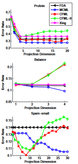


FDA Goals
An intuitive description of FDA can be given by visualizing two clouds of data, as shown above. Ideally, we would like to collapse all of the data points in each cloud onto one point on some projected line, then make those two points as far apart as possible. In doing so, we make it very easy to tell which class a data point belongs to. In practice, it is not possible to collapse all of the points in a cloud to one point, but we attempt to make all of the points in a cloud close to each other while simultaneously far from the points in the other cloud.
Example in R

>> X = matrix(nrow=400,ncol=2)
>> X[1:200,] = mvrnorm(n=200,mu=c(1,1),Sigma=matrix(c(1,1.5,1.5,3),2))
>> X[201:400,] = mvrnorm(n=200,mu=c(5,3),Sigma=matrix(c(1,1.5,1.5,3),2))
>> Y = c(rep("red",200),rep("blue",200))
- Create 2 multivariate normal random variables with [math]\displaystyle{ \, \mu_1 = \left( \begin{array}{c}1 \\ 1 \end{array} \right), \mu_2 = \left( \begin{array}{c}5 \\ 3 \end{array} \right). ~\textrm{Cov} = \left( \begin{array}{cc} 1 & 1.5 \\ 1.5 & 3 \end{array} \right) }[/math]. Create
Y, an index indicating which class they belong to.
>> s <- svd(X,nu=1,nv=1)
- Calculate the singular value decomposition of X. The most significant direction is in
s$v[,1], and is displayed as a black line.
>> s2 <- lda(X,grouping=Y)
- The
ldafunction, given the group for each item, uses Fischer's Linear Discriminant Analysis (FLDA) to find the most discriminant direction. This can be found ins2$scaling.
Now that we've calculated the PCA and FLDA decompositions, we create a plot to demonstrate the differences between the two algorithms. FLDA is clearly better suited to discriminating between two classes whereas PCA is primarily good for reducing the number of dimensions when data is high-dimensional.
>> plot(X,col=Y,main="PCA vs. FDA example")
- Plot the set of points, according to colours given in Y.
>> slope = s$v[2]/s$v[1]
>> intercept = mean(X[,2])-slope*mean(X[,1])
>> abline(a=intercept,b=slope)
- Plot the main PCA direction, drawn through the mean of the dataset. Only the direction is significant.
>> slope2 = s2$scaling[2]/s2$scaling[1]
>> intercept2 = mean(X[,2])-slope2*mean(X[,1])
>> abline(a=intercept2,b=slope2,col="red")
- Plot the FLDA direction, again through the mean.
>> legend(-2,7,legend=c("PCA","FDA"),col=c("black","red"),lty=1)
- Labeling the lines directly on the graph makes it easier to interpret.
FDA projects the data into lower dimensional space, where the distances between the projected means are maximum and the within-class variances are minimum. There are two categories of classification problems:
1. Two-class problem
2. Multi-class problem (addressed next lecture)
Two-class problem
In the two-class problem, we have prior knowledge that the data points belong to two classes. Conceptually, points of each class form a cloud around the class mean, and each class has an distinct size. To divide points among the two classes, we must determine the class whose mean is closest to each point, and we must also account for the different size of each class given by the covariance of each class.
Assume [math]\displaystyle{ \underline{\mu_{1}}=\frac{1}{n_{1}}\displaystyle\sum_{i:y_{i}=1}\underline{x_{i}} }[/math] and [math]\displaystyle{ \displaystyle\Sigma_{1} }[/math], represent the mean and covariance of the 1st class, and [math]\displaystyle{ \underline{\mu_{2}}=\frac{1}{n_{2}}\displaystyle\sum_{i:y_{i}=2}\underline{x_{i}} }[/math] and [math]\displaystyle{ \displaystyle\Sigma_{2} }[/math] represent the mean and covariance of the 2nd class. We have to find a transformation which satisfies the following goals:
1.To make the means of these two classes as far apart as possible
- In other words, the goal is to maximize the distance after projection between class 1 and class 2. This can be done by maximizing the distance between the means of the classes after projection. When projecting the data points to a one-dimensional space, all points will be projected to a single line; the line we seek is the one with the direction that achieves maximum separation of classes upon projection. If the original points are [math]\displaystyle{ \underline{x_{i}} \in \mathbb{R}^{d} }[/math]and the projected points are [math]\displaystyle{ \underline{w}^T \underline{x_{i}} }[/math] then the mean of the projected points will be [math]\displaystyle{ \underline{w}^T \underline{\mu_{1}} }[/math] and [math]\displaystyle{ \underline{w}^T \underline{\mu_{2}} }[/math] for class 1 and class 2 respectively. The goal now becomes to maximize the Euclidean distance between projected means, [math]\displaystyle{ (\underline{w}^T\underline{\mu_{1}}-\underline{w}^T\underline{\mu_{2}})^T (\underline{w}^T\underline{\mu_{1}}-\underline{w}^T\underline{\mu_{2}}) }[/math]. The steps of this maximization are given below.
2.We want to collapse all data points of each class to a single point, i.e., minimize the covariance within each class
- Notice that the variance of the projected classes 1 and 2 are given by [math]\displaystyle{ \underline{w}^T\Sigma_{1}\underline{w} }[/math] and [math]\displaystyle{ \underline{w}^T\Sigma_{2}\underline{w} }[/math]. The second goal is to minimize the sum of these two covariances (the summation of the two covariances is a valid covariance, satisfying the symmetry and positive semi-definite criteria).
{{
Template:namespace detect
| type = style | image = | imageright = | style = | textstyle = | text = This article may require cleanup to meet Wikicoursenote's quality standards. The specific problem is: In 2. above, I wonder if the computation would be much more complex if we instead find a weighted sum of the covariances of the two classes where the weights are the sizes of the two classes?. Please improve this article if you can. (October 2010) | small = | smallimage = | smallimageright = | smalltext = }}
{{
Template:namespace detect
| type = style | image = | imageright = | style = | textstyle = | text = This article may require cleanup to meet Wikicoursenote's quality standards. The specific problem is: If using the weighted sum of two covariances, you will need to use the shared mean of the two classes, and the weighted sum will be the shared covariance. Doing this will result in collapsing the two classes into one point, which contradicts the purpose of using FDA. Please improve this article if you can. (December 2010) | small = | smallimage = | smallimageright = | smalltext = }}
As is demonstrated below, both of these goals can be accomplished simultaneously.
Original points are [math]\displaystyle{ \underline{x_{i}} \in \mathbb{R}^{d} }[/math]
[math]\displaystyle{ \ \{ \underline x_1 \underline x_2 \cdot \cdot \cdot \underline x_n \} }[/math]
Projected points are [math]\displaystyle{ \underline{z_{i}} \in \mathbb{R}^{1} }[/math] with [math]\displaystyle{ \underline{z_{i}} = \underline{w}^T \cdot\underline{x_{i}} }[/math] where [math]\displaystyle{ \ z_i }[/math] is a scalar
1. Minimizing within-class variance
[math]\displaystyle{ \displaystyle \min_w (\underline{w}^T\sum_1\underline{w}) }[/math]
[math]\displaystyle{ \displaystyle \min_w (\underline{w}^T\sum_2\underline{w}) }[/math]
and this problem reduces to [math]\displaystyle{ \displaystyle \min_w (\underline{w}^T(\sum_1 + \sum_2)\underline{w}) }[/math]
(where [math]\displaystyle{ \,\sum_1 }[/math] and [math]\displaystyle{ \,\sum_2 }[/math] are the covariance matrices of the 1st and 2nd classes of data, respectively)
Let [math]\displaystyle{ \displaystyle \ s_w=\sum_1 + \sum_2 }[/math] be the within-classes covariance. Then, this problem can be rewritten as [math]\displaystyle{ \displaystyle \min_w (\underline{w}^Ts_w\underline{w}) }[/math].
2. Maximize the distance between the means of the projected data
[math]\displaystyle{ \displaystyle \max_w ||\underline{w}^T \mu_1 - \underline{w}^T \mu_2||^2, }[/math]
[math]\displaystyle{ \begin{align} ||\underline{w}^T \mu_1 - \underline{w}^T \mu_2||^2 &= (\underline{w}^T \mu_1 - \underline{w}^T \mu_2)^T(\underline{w}^T \mu_1 - \underline{w}^T \mu_2)\\
&= (\mu_1^T\underline{w} - \mu_2^T\underline{w})(\underline{w}^T \mu_1 - \underline{w}^T \mu_2)\\
&= (\mu_1 - \mu_2)^T \underline{w} \underline{w}^T (\mu_1 - \mu_2) \\
&= ((\mu_1 - \mu_2)^T \underline{w})^{T} (\underline{w}^T (\mu_1 - \mu_2))^{T} \\
&= \underline{w}^T(\mu_1 - \mu_2)(\mu_1 - \mu_2)^T \underline{w} \end{align} }[/math]
Note that in the last line above the order is rearranged clockwise because the answer is a scalar.
Let [math]\displaystyle{ \displaystyle s_B = (\mu_1 - \mu_2)(\mu_1 - \mu_2)^T }[/math], the between-class covariance, then the goal is to [math]\displaystyle{ \displaystyle \max_w (\underline{w}^T(\mu_1 - \mu_2)(\mu_1 - \mu_2)^T\underline{w}) }[/math] or [math]\displaystyle{ \displaystyle \max_w (\underline{w}^Ts_B\underline{w}) }[/math].
The Objective Function for FDA
We want an objective function which satisfies both of the goals outlined above (at the same time).
- [math]\displaystyle{ \displaystyle \min_w (\underline{w}^T(\sum_1 + \sum_2)\underline{w}) }[/math] or [math]\displaystyle{ \displaystyle \min_w (\underline{w}^Ts_w\underline{w}) }[/math]
- [math]\displaystyle{ \displaystyle \max_w (\underline{w}^T(\mu_1 - \mu_2)(\mu_1 - \mu_2)^T\underline{w}) }[/math] or [math]\displaystyle{ \displaystyle \max_w (\underline{w}^Ts_B\underline{w}) }[/math]
So, we construct our objective function as maximizing the ratio of the two goals brought above:
[math]\displaystyle{ \displaystyle \max_w \frac{(\underline{w}^T(\mu_1 - \mu_2)(\mu_1 - \mu_2)^T\underline{w})} {(\underline{w}^T(\sum_1 + \sum_2)\underline{w})} }[/math]
or equivalently,
[math]\displaystyle{ \displaystyle \max_w \frac{(\underline{w}^Ts_B\underline{w})}{(\underline{w}^Ts_w\underline{w})} }[/math]
One may argue that we can use subtraction for this purpose, while this approach is true but it can be shown it will need another scaling factor. Thus using this ratio is more efficient.
As the objective function is convex, and so it does not have a maximum. To get around this problem, we have to add the constraint that w must have unit length, and then solvethis optimization problem we form the lagrangian:
[math]\displaystyle{ \displaystyle L(\underline{w},\lambda) = \underline{w}^Ts_B\underline{w} - \lambda (\underline{w}^Ts_w\underline{w} -1) }[/math]
Then, we equate the partial derivative of L with respect to [math]\displaystyle{ \underline{w} }[/math]:
[math]\displaystyle{ \displaystyle \frac{\partial L}{\partial \underline{w}}=2s_B \underline{w} - 2\lambda s_w \underline{w} = 0 }[/math]
[math]\displaystyle{ s_B \underline{w} = \lambda s_w \underline{w} }[/math]
[math]\displaystyle{ s_w^{-1}s_B \underline{w}= \lambda\underline{w} }[/math]
This is in the form of generalized eigenvalue problem. Therefore, [math]\displaystyle{ \underline{w} }[/math] is the largest eigenvector of [math]\displaystyle{ s_w^{-1}s_B }[/math]
This solution can be further simplified as follow:
[math]\displaystyle{ s_w^{-1}(\mu_1 - \mu_2)(\mu_1 - \mu_2)^T\underline{w} = \lambda\underline{w} }[/math]
Since [math]\displaystyle{ (\mu_1 - \mu_2)^T\underline{w} }[/math] is a scalar then [math]\displaystyle{ s_w^{-1}(\mu_1 - \mu_2) }[/math]∝[math]\displaystyle{ \underline{w} }[/math]
This gives the direction of [math]\displaystyle{ \underline{w} }[/math] without doing eigenvalue decomposition in the case of 2-class problem.
Note: In order for [math]\displaystyle{ {s_w} }[/math] to have an inverse, it must have full rank. This can be achieved by ensuring that the number of data points [math]\displaystyle{ \,\ge }[/math] the dimensionality of [math]\displaystyle{ \underline{x_{i}} }[/math].
FDA Using Matlab
Note: The following example was not actually mentioned in this lecture
We see now an application of the theory that we just introduced. Using Matlab, we find the principal components and the projection by Fisher Discriminant Analysis of two Bivariate normal distributions to show the difference between the two methods.
      %First of all, we generate the two data set:
      % First data set X1
      X1 = mvnrnd([1,1],[1 1.5; 1.5 3], 300);
      %In this case:
      mu_1=[1;1];
      Sigma_1=[1 1.5; 1.5 3];
      %where mu and sigma are the mean and covariance matrix.
      % Second data set X2
      X2 = mvnrnd([5,3],[1 1.5; 1.5 3], 300);
      %Here mu_2=[5;3] and Sigma_2=[1 1.5; 1.5 3]
      %The plot of the two distributions is:
      plot(X1(:,1),X1(:,2),'.b'); hold on;
      plot(X2(:,1),X2(:,2),'ob')

      %We compute the principal components:
      % Combine data sets to map both into the same subspace
      X=[X1;X2];
      X=X';
      % We used built-in PCA function in Matlab
      [coefs, scores]=princomp(X);

      plot([0 coefs(1,1)], [0 coefs(2,1)],'b')
      plot([0 coefs(1,1)]*10, [0 coefs(2,1)]*10,'r')
      sw=2*[1 1.5;1.5 3]   % sw=Sigma1+Sigma2=2*Sigma1
      w=sw\[4; 2]       % calculate s_w^{-1}(mu2 - mu1)
      plot ([0 w(1)], [0 w(2)],'g')

      %We now make the projection:
      Xf=w'*X
      figure
      plot(Xf(1:300),1,'ob') %In this case, since it's a one dimension data, the plot is "Data Vs Indexes"
      hold on
      plot(Xf(301:600),1,'or')

      %We see that in the above picture that there is very little overlapping
      Xp=coefs(:,1)'*X
      figure
      plot(Xp(1:300),1,'b')
      hold on
      plot(Xp(301:600),2,'or')

%In this case there is an overlapping since we project the first principal component on [Xp=coefs(:,1)'*X]
Some of FDA applications
There are many applications for FDA in many domains; a few examples are stated below:
- Speech/Music/Noise Classification in Hearing Aids
FDA can be used to enhance listening comprehension when the user goes from one sound environment to another different one. In practice, many people who require hearing aids do not wear them due in part to the nusiance of having to adjust the settings each time a user changes noise environments (for example, from a quiet walk in the to park to a crowded cafe). If the hearing aid itself could distinguish between the type of sound environment and automatically adjust its settings itself, many more people may be willing to wear and use the hearing aids. The paper referenced below examines the difference in using a classifier based on one level and three classes ("speech", "noisy" or "music" environments) and a classifier based on two levels with two classes each ("speech" versus "non-speech" and then for the "non-speech" group, between "noisy" and "music") and also includes a discussion about the feasibility of implementing these classifiers in the hearing aids. For more information review this paper by Alexandre et al. here.
- Application to Face Recognition
FDA can be used in face recognition for different situations. Instead of using the one-dimensional LDA where the data is transformed into long column vectors with less-than-full-rank covariance matrices for the within-class and between-class covariance matrices, several other approaches of using FDA are suggested here including a two-dimensional approach where the data is stored as a matrix rather than a column vector. In this case, the covariance matrices are full-rank. Details can be found in the paper by Kong et al. here.
- Palmprint Recognition
FDA is used in biometrics to implement an automated palmprint recognition system. In Tee et al. here An Automated Palmprint Recognition System was proposed and FDA was used to match images in a compressed subspace where these subspaces best discriminate among classes. It is different from PCA in the aspect that it deals directly with class separation while PCA treats images in its entirety without considering the underlying class structure.
- Other Applications
Other applications can be seen in [4] where FDA was used to authenticate different olive oil types, or classify multiple fault classes [5]. As well as, applications on face recognition [6] and shape deformations to localize epilepsy [8].
References
1. Kong, H.; Wang, L.; Teoh, E.K.; Wang, J.-G.; Venkateswarlu, R.; , "A framework of 2D Fisher discriminant analysis: application to face recognition with small number of training samples," Computer Vision and Pattern Recognition, 2005. CVPR 2005. IEEE Computer Society Conference on , vol.2, no., pp. 1083- 1088 vol. 2, 20-25 June 2005 doi: 10.1109/CVPR.2005.30 1
2. Enrique Alexandre, Roberto Gil-Pita, Lucas Cuadra, Lorena A´lvarez, Manuel Rosa-Zurera, "SPEECH/MUSIC/NOISE CLASSIFICATION IN HEARING AIDS USING A TWO-LAYER CLASSIFICATION SYSTEM WITH MSE LINEAR DISCRIMINANTS", 16th European Signal Processing Conference (EUSIPCO 2008), Lausanne, Switzerland, August 25-29, 2008, copyright by EURASIP, 2
3. Connie, Tee; Jin, Andrew Teoh Beng; Ong, Michael Goh Kah; Ling, David Ngo Chek; "An automated palmprint recognition system", Journal of Image and Vision Computing, 2005. 3
4. met, Francesca; Boqué, Ricard; Ferré, Joan; "Application of non-negative matrix factorization combined with Fisher's linear discriminant analysis for classification of olive oil excitation-emission fluorescence spectra", Journal of Chemometrics and Intelligent Laboratory Systems, 2006. 4
5. Chiang, Leo H.;Kotanchek, Mark E.;Kordon, Arthur K.; "Fault diagnosis based on Fisher discriminant analysis and support vector machines" Journal of Computers & Chemical Engineering, 2004 5
6. Yang, Jian ;Frangi, Alejandro F.; Yang, Jing-yu; "A new kernel Fisher discriminant algorithm with application to face recognition", 2004 6
7. Cawley, Gavin C.; Talbot, Nicola L. C.; "Efficient leave-one-out cross-validation of kernel fisher discriminant classifiers", Journal of Pattern Recognition , 2003 7
8. Kodipaka, S.; Vemuri, B.C.; Rangarajan, A.; Leonard, C.M.; Schmallfuss, I.; Eisenschenk, S.; "Kernel Fisher discriminant for shape-based classification in epilepsy" Hournal Medical Image Analysis, 2007. 8
9. Fisher LDA and Kernel Fisher LDA [26]
Fisher's (Linear) Discriminant Analysis (FDA) - Multi-Class Problem - October 7, 2010
Obtaining Covariance Matrices
The within-class covariance matrix [math]\displaystyle{ \mathbf{S}_{W} }[/math] is easy to obtain:
- [math]\displaystyle{ \begin{align} \mathbf{S}_{W} = \sum_{i=1}^{k} \mathbf{S}_{i} \end{align} }[/math]
where [math]\displaystyle{ \mathbf{S}_{i} = \frac{1}{n_{i}}\sum_{j: y_{j}=i}(\mathbf{x}_{j} - \mathbf{\mu}_{i})(\mathbf{x}_{j} - \mathbf{\mu}_{i})^{T} }[/math] and [math]\displaystyle{ \mathbf{\mu}_{i} = \frac{\sum_{j: y_{j}=i}\mathbf{x}_{j}}{n_{i}} }[/math].
However, the between-class covariance matrix [math]\displaystyle{ \mathbf{S}_{B} }[/math] is not easy to compute directly. To bypass this problem we use the following method. We know that the total covariance [math]\displaystyle{ \,\mathbf{S}_{T} }[/math] of a given set of data is constant and known, and we can also decompose this variance into two parts: the within-class variance [math]\displaystyle{ \mathbf{S}_{W} }[/math] and the between-class variance [math]\displaystyle{ \mathbf{S}_{B} }[/math] in a way that is similar to ANOVA. We thus have:
- [math]\displaystyle{ \begin{align} \mathbf{S}_{T} = \mathbf{S}_{W} + \mathbf{S}_{B} \end{align} }[/math]
where the total variance is given by
- [math]\displaystyle{ \begin{align} \mathbf{S}_{T} = \frac{1}{n} \sum_{i}(\mathbf{x_{i}-\mu})(\mathbf{x_{i}-\mu})^{T} \end{align} }[/math]
We can now get [math]\displaystyle{ \mathbf{S}_{B} }[/math] from the relationship:
- [math]\displaystyle{ \begin{align} \mathbf{S}_{B} = \mathbf{S}_{T} - \mathbf{S}_{W} \end{align} }[/math]
Actually, there is another way to obtain [math]\displaystyle{ \mathbf{S}_{B} }[/math]. Suppose the data contains [math]\displaystyle{ \, k }[/math] classes, and each class [math]\displaystyle{ \, j }[/math] contains [math]\displaystyle{ \, n_{j} }[/math] data points. We denote the overall mean vector by
- [math]\displaystyle{ \begin{align} \mathbf{\mu} = \frac{1}{n}\sum_{i}\mathbf{x_{i}} = \frac{1}{n}\sum_{j=1}^{k}n_{j}\mathbf{\mu}_{j} \end{align} }[/math]
Thus the total covariance matrix [math]\displaystyle{ \mathbf{S}_{T} }[/math] is
- [math]\displaystyle{ \begin{align} \mathbf{S}_{T} = \frac{1}{n} \sum_{i}(\mathbf{x_{i}-\mu})(\mathbf{x_{i}-\mu})^{T} \end{align} }[/math]
Thus we obtain
- [math]\displaystyle{ \begin{align} & \mathbf{S}_{T} = \sum_{i=1}^{k}\sum_{j: y_{j}=i}(\mathbf{x}_{j} - \mathbf{\mu}_{i} + \mathbf{\mu}_{i} - \mathbf{\mu})(\mathbf{x}_{j} - \mathbf{\mu}_{i} + \mathbf{\mu}_{i} - \mathbf{\mu})^{T} \\& = \sum_{i=1}^{k}\sum_{j: y_{j}=i}(\mathbf{x}_{j}-\mathbf{\mu}_{i})(\mathbf{x}_{j}-\mathbf{\mu}_{i})^{T}+ \sum_{i=1}^{k}\sum_{j: y_{j}=i}(\mathbf{\mu}_{i}-\mathbf{\mu})(\mathbf{\mu}_{i}-\mathbf{\mu})^{T} \\& = \mathbf{S}_{W} + \sum_{i=1}^{k} n_{i}(\mathbf{\mu}_{i}-\mathbf{\mu})(\mathbf{\mu}_{i}-\mathbf{\mu})^{T} \end{align} }[/math]
Since the total covariance [math]\displaystyle{ \mathbf{S}_{T} }[/math] is the sum of the within-class covariance [math]\displaystyle{ \mathbf{S}_{W} }[/math] and the between-class covariance [math]\displaystyle{ \mathbf{S}_{B} }[/math], we can denote the second term in the final line of the derivation above as the between-class covariance matrix [math]\displaystyle{ \mathbf{S}_{B} }[/math], thus we obtain
- [math]\displaystyle{ \begin{align} \mathbf{S}_{B} = \sum_{i=1}^{k} n_{i}(\mathbf{\mu}_{i}-\mathbf{\mu})(\mathbf{\mu}_{i}-\mathbf{\mu})^{T} \end{align} }[/math]
Recall that in the two class case problem, we have
- [math]\displaystyle{ \begin{align} & \mathbf{S}_{B}^* = (\mathbf{\mu}_{1}-\mathbf{\mu}_{2})(\mathbf{\mu}_{1}-\mathbf{\mu}_{2})^{T} \\ & = (\mathbf{\mu}_{1}-\mathbf{\mu}+\mathbf{\mu}-\mathbf{\mu}_{2})(\mathbf{\mu}_{1}-\mathbf{\mu}+\mathbf{\mu}-\mathbf{\mu}_{2})^{T} \\ & = ((\mathbf{\mu}_{1}-\mathbf{\mu})-(\mathbf{\mu}_{2}-\mathbf{\mu}))((\mathbf{\mu}_{1}-\mathbf{\mu})-(\mathbf{\mu}_{2}-\mathbf{\mu}))^{T} \\ & = ((\mathbf{\mu}_{1}-\mathbf{\mu})-(\mathbf{\mu}_{2}-\mathbf{\mu}))((\mathbf{\mu}_{1}-\mathbf{\mu})^{T}-(\mathbf{\mu}_{2}-\mathbf{\mu})^{T}) \\ & = (\mathbf{\mu}_{1}-\mathbf{\mu})(\mathbf{\mu}_{1}-\mathbf{\mu})^{T}-(\mathbf{\mu}_{1}-\mathbf{\mu})(\mathbf{\mu}_{2}-\mathbf{\mu})^{T}-(\mathbf{\mu}_{2}-\mathbf{\mu})(\mathbf{\mu}_{1}-\mathbf{\mu})^{T}+(\mathbf{\mu}_{2}-\mathbf{\mu})(\mathbf{\mu}_{2}-\mathbf{\mu})^{T} \end{align} }[/math]
- [math]\displaystyle{ \begin{align} & \mathbf{S}_{B} = n_{1}(\mathbf{\mu}_{1}-\mathbf{\mu})(\mathbf{\mu}_{1}-\mathbf{\mu})^{T} + n_{2}(\mathbf{\mu}_{2}-\mathbf{\mu})(\mathbf{\mu}_{2}-\mathbf{\mu})^{T} \end{align} }[/math]
Apparently, they are very similar.
Now, we are trying to find the optimal transformation. Basically, we have
- [math]\displaystyle{ \begin{align} \mathbf{z}_{i} = \mathbf{W}^{T}\mathbf{x}_{i}, i=1,2,...,k-1 \end{align} }[/math]
where [math]\displaystyle{ \mathbf{z}_{i} }[/math] is a [math]\displaystyle{ (k-1)\times 1 }[/math] vector, [math]\displaystyle{ \mathbf{W} }[/math] is a [math]\displaystyle{ d\times (k-1) }[/math] transformation matrix, i.e. [math]\displaystyle{ \mathbf{W} = [\mathbf{w}_{1}, \mathbf{w}_{2},..., \mathbf{w}_{k-1}] }[/math], and [math]\displaystyle{ \mathbf{x}_{i} }[/math] is a [math]\displaystyle{ d\times 1 }[/math] column vector.
Thus we obtain
- [math]\displaystyle{ \begin{align} & \mathbf{S}_{W}^{\ast} = \sum_{i=1}^{k}\sum_{j: y_{j}=i}(\mathbf{W}^{T}\mathbf{x}_{j}-\mathbf{W}^{T}\mathbf{\mu}_{i})(\mathbf{W}^{T}\mathbf{x}_{j}-\mathbf{W}^{T}\mathbf{\mu}_{i})^{T} \\ & = \sum_{i=1}^{k}\sum_{j: y_{j}=i}(\mathbf{W}^{T}(\mathbf{x}_{j}-\mathbf{\mu}_{i}))(\mathbf{W}^{T}(\mathbf{x}_{j}-\mathbf{\mu}_{i}))^{T} \\ & = \sum_{i=1}^{k}\sum_{j: y_{j}=i}(\mathbf{W}^{T}(\mathbf{x}_{j}-\mathbf{\mu}_{i}))((\mathbf{x}_{j}-\mathbf{\mu}_{i})^{T}\mathbf{W}) \\ & = \sum_{i=1}^{k}\sum_{j: y_{j}=i}\mathbf{W}^{T}(\mathbf{x}_{j}-\mathbf{\mu}_{i})(\mathbf{x}_{j}-\mathbf{\mu}_{i})^{T}\mathbf{W} \\ & = \mathbf{W}^{T}\left[\sum_{i=1}^{k}\sum_{j: y_{j}=i}(\mathbf{x}_{j}-\mathbf{\mu}_{i})(\mathbf{x}_{j}-\mathbf{\mu}_{i})^{T}\right]\mathbf{W} \\ & = \mathbf{W}^{T}\mathbf{S}_{W}\mathbf{W} \end{align} }[/math]
Similarly, we obtain
- [math]\displaystyle{ \begin{align} & \mathbf{S}_{B}^{\ast} = \sum_{i=1}^{k}n_{i}(\mathbf{W}^{T}\mathbf{\mu}_{i}-\mathbf{W}^{T}\mathbf{\mu})(\mathbf{W}^{T}\mathbf{\mu}_{i}-\mathbf{W}^{T}\mathbf{\mu})^{T} \\ & = \sum_{i=1}^{k}n_{i}\mathbf{W}^{T}(\mathbf{\mu}_{i}-\mathbf{\mu})(\mathbf{\mu}_{i}-\mathbf{\mu})^{T}\mathbf{W} \\ & = \mathbf{W}^{T}\left[ \sum_{i=1}^{k}n_{i}(\mathbf{\mu}_{i}-\mathbf{\mu})(\mathbf{\mu}_{i}-\mathbf{\mu})^{T}\right]\mathbf{W} \\ & = \mathbf{W}^{T}\mathbf{S}_{B}\mathbf{W} \end{align} }[/math]
Now, we use the following as our measure:
- [math]\displaystyle{ \begin{align} \sum_{i=1}^{k}n_{i}\|(\mathbf{W}^{T}\mathbf{\mu}_{i}-\mathbf{W}^{T}\mathbf{\mu})^{T}\|^{2} \end{align} }[/math]
The solution for this question is that the columns of the transformation matrix [math]\displaystyle{ \mathbf{W} }[/math] are exactly the eigenvectors that correspond to the largest [math]\displaystyle{ k-1 }[/math] eigenvalues with respect to
{{
Template:namespace detect
| type = style | image = | imageright = | style = | textstyle = | text = This article may require cleanup to meet Wikicoursenote's quality standards. The specific problem is: What if we encounter complex eigenvalues? Then concept of being large does not dense. What is the solution in that case?. Please improve this article if you can. | small = | smallimage = | smallimageright = | smalltext = }} {{
Template:namespace detect
| type = style | image = | imageright = | style = | textstyle = | text = This article may require cleanup to meet Wikicoursenote's quality standards. The specific problem is: Covariance matrices are positive semi-definite. The inverse of a positive semi-definite matrix is positive semi-definite. The product of positive semi-definite matrices is positive semi-definite. The eigenvalues of a positive semi-definite matrix are all real, non-negative values. As a result, the eigenvalues of \mathbf{S}_{W}^{-1}\mathbf{S}_{B} will always be real, non-negative values.. Please improve this article if you can. (December 2010) | small = | smallimage = | smallimageright = | smalltext = }}
- [math]\displaystyle{ \begin{align} \mathbf{S}_{W}^{-1}\mathbf{S}_{B}\mathbf{w}_{i} = \lambda_{i}\mathbf{w}_{i} \end{align} }[/math]
Recall that the Frobenius norm of [math]\displaystyle{ X }[/math] is
- [math]\displaystyle{ \begin{align} \|\mathbf{X}\|^2_{2} = Tr(\mathbf{X}^{T}\mathbf{X}) \end{align} }[/math]
- [math]\displaystyle{ \begin{align} & \sum_{i=1}^{k}n_{i}\|(\mathbf{W}^{T}\mathbf{\mu}_{i}-\mathbf{W}^{T}\mathbf{\mu})^{T}\|^{2} \\ & = \sum_{i=1}^{k}n_{i}Tr[(\mathbf{W}^{T}\mathbf{\mu}_{i}-\mathbf{W}^{T}\mathbf{\mu})(\mathbf{W}^{T}\mathbf{\mu}_{i}-\mathbf{W}^{T}\mathbf{\mu})^{T}] \\ & = Tr[\sum_{i=1}^{k}n_{i}(\mathbf{W}^{T}\mathbf{\mu}_{i}-\mathbf{W}^{T}\mathbf{\mu})(\mathbf{W}^{T}\mathbf{\mu}_{i}-\mathbf{W}^{T}\mathbf{\mu})^{T}] \\ & = Tr[\sum_{i=1}^{k}n_{i}\mathbf{W}^{T}(\mathbf{\mu}_{i}-\mathbf{\mu})(\mathbf{\mu}_{i}-\mathbf{\mu})^{T}\mathbf{W}] \\ & = Tr[\mathbf{W}^{T}\sum_{i=1}^{k}n_{i}(\mathbf{\mu}_{i}-\mathbf{\mu})(\mathbf{\mu}_{i}-\mathbf{\mu})^{T}\mathbf{W}] \\ & = Tr[\mathbf{W}^{T}\mathbf{S}_{B}\mathbf{W}] \end{align} }[/math]
Similarly, we can get [math]\displaystyle{ Tr[\mathbf{W}^{T}\mathbf{S}_{W}\mathbf{W}] }[/math]. Thus we have the following classic criterion function that Fisher used
- [math]\displaystyle{ \begin{align} \phi(\mathbf{W}) = \frac{Tr[\mathbf{W}^{T}\mathbf{S}_{B}\mathbf{W}]}{Tr[\mathbf{W}^{T}\mathbf{S}_{W}\mathbf{W}]} \end{align} }[/math]
Similar to the two class case problem, we have:
max [math]\displaystyle{ Tr[\mathbf{W}^{T}\mathbf{S}_{B}\mathbf{W}] }[/math] subject to [math]\displaystyle{ Tr[\mathbf{W}^{T}\mathbf{S}_{W}\mathbf{W}]=1 }[/math]
To solve this optimization problem a Lagrange multiplier [math]\displaystyle{ \Lambda }[/math], which actually is a [math]\displaystyle{ d \times d }[/math] diagonal matrix, is introduced:
- [math]\displaystyle{ \begin{align} L(\mathbf{W},\Lambda) = Tr[\mathbf{W}^{T}\mathbf{S}_{B}\mathbf{W}] - \Lambda\left\{ Tr[\mathbf{W}^{T}\mathbf{S}_{W}\mathbf{W}] - 1 \right\} \end{align} }[/math]
Differentiating with respect to [math]\displaystyle{ \mathbf{W} }[/math] we obtain:
- [math]\displaystyle{ \begin{align} \frac{\partial L}{\partial \mathbf{W}} = (\mathbf{S}_{B} + \mathbf{S}_{B}^{T})\mathbf{W} - \Lambda (\mathbf{S}_{W} + \mathbf{S}_{W}^{T})\mathbf{W} \end{align} }[/math]
Note that the [math]\displaystyle{ \mathbf{S}_{B} }[/math] and [math]\displaystyle{ \mathbf{S}_{W} }[/math] are both symmetric matrices, thus set the first derivative to zero, we obtain:
- [math]\displaystyle{ \begin{align} \mathbf{S}_{B}\mathbf{W} - \Lambda\mathbf{S}_{W}\mathbf{W}=0 \end{align} }[/math]
Thus,
- [math]\displaystyle{ \begin{align} \mathbf{S}_{B}\mathbf{W} = \Lambda\mathbf{S}_{W}\mathbf{W} \end{align} }[/math]
where
- [math]\displaystyle{ \mathbf{\Lambda} = \begin{pmatrix} \lambda_{1} & & 0\\ &\ddots&\\ 0 & &\lambda_{d} \end{pmatrix} }[/math]
and [math]\displaystyle{ \mathbf{W} = [\mathbf{w}_{1}, \mathbf{w}_{2},..., \mathbf{w}_{k-1}] }[/math].
As a matter of fact, [math]\displaystyle{ \mathbf{\Lambda} }[/math] must have [math]\displaystyle{ \mathbf{k-1} }[/math] nonzero eigenvalues, because [math]\displaystyle{ rank({S}_{W}^{-1}\mathbf{S}_{B})=k-1 }[/math].
Therefore, the solution for this question is as same as the previous case. The columns of the transformation matrix [math]\displaystyle{ \mathbf{W} }[/math] are exactly the eigenvectors that correspond to the largest [math]\displaystyle{ k-1 }[/math] eigenvalues with respect to
- [math]\displaystyle{ \begin{align} \mathbf{S}_{W}^{-1}\mathbf{S}_{B}\mathbf{w}_{i} = \lambda_{i}\mathbf{w}_{i} \end{align} }[/math]
{{
Template:namespace detect
| type = style | image = | imageright = | style = | textstyle = | text = This article may require cleanup to meet Wikicoursenote's quality standards. The specific problem is: Adding more general comments about the advantages and flaws of FDA would be effective here.. Please improve this article if you can. (October 2010) | small = | smallimage = | smallimageright = | smalltext = }}
{{
Template:namespace detect
| type = style | image = | imageright = | style = | textstyle = | text = This article may require cleanup to meet Wikicoursenote's quality standards. The specific problem is: Would you please show how could we reconstruct our original data from the data that its dimentionality is reduced by FDA.. Please improve this article if you can. (October 2010) | small = | smallimage = | smallimageright = | smalltext = }} {{
Template:namespace detect
| type = style | image = | imageright = | style = | textstyle = | text = This article may require cleanup to meet Wikicoursenote's quality standards. The specific problem is: When you reduce the dimensionality of data in most general form you lose some features of the data and you cannot reconstruct the data from redacted space unless the data have special features that help you in reconstruction like sparsity. In FDA it seems that we cannot reconstruct data in general form using reducted version of data. Please improve this article if you can. (October 2010) | small = | smallimage = | smallimageright = | smalltext = }}
Advantages of FDA compared with PCA
-PCA find components which are useful for representing data.
-While there is no reason to assume that components are useful to discriminate data between classes.
-In FDA , we try to use labels to find the components which are useful for discriminating data.
Generalization of Fisher's Linear Discriminant Analysis
Fisher's Linear Discriminant Analysis (Fisher, 1936) is very popular among users of discriminant analysis. Some of the reasons for this are its simplicity and lack of necessity for strict assumptions. However, it has optimality properties only if the underlying distributions of the groups are multivariate normal. It is also easy to verify that the discriminant rule obtained can be very harmed by only a small number of outlying observations. Outliers are very hard to detect in multivariate data sets and even when they are detected simply discarding them is not the most efficient way of handling the situation. Therefore, there is a need for robust procedures that can accommodate the outliers and are not strongly affected by them. Then, a generalization of Fisher's linear discriminant algorithm [[27]] is developed to lead easily to a very robust procedure.
Also notice that LDA can be seen as a dimensionality reduction technique. In general k-class problems, we have k means which lie on a linear subspace with dimension k-1. Given a data point, we are looking for the closest class mean to this point. In LDA, we project the data point to the linear subspace and calculate distances within that subspace. If the dimensionality of the data, d, is much larger than the number of classes, k, then we have a considerable drop in dimensionality from d dimensions to k - 1 dimensions.
Multiple Discriminant Analysis
(MDA) is also termed Discriminant Factor Analysis and Canonical Discriminant Analysis. It adopts a similar perspective to PCA: the rows of the data matrix to be examined constitute points in a multidimensional space, as also do the group mean vectors. Discriminating axes are determined in this space, in such a way that optimal separation of the predefined groups is attained. As with PCA, the problem becomes mathematically the eigenreduction of a real, symmetric matrix. The eigenvalues represent the discriminating power of the associated eigenvectors. The nYgroups lie in a space of dimension at most [math]\displaystyle{ n_{y-1} }[/math]. This will be the number of discriminant axes or factors obtainable in the most common practical case when n > m > nY (where n is the number of rows, and m the number of columns of the input data matrix.
Matlab Example: Multiple Discriminant Analysis for Face Recognition
% The following MATLAB code is an example of using MDA in face recognition. The used dataset can be % found be found here. IT contains % a set of face images taken between April 1992 and April 1994 at the lab. The database was used in the % context of a face recognition project carried out in collaboration with the Speech, Vision and % Robotics Group of the Cambridge University Engineering Department.
load orl_faces_112x92.mat
u=(mean(faces'))';
stfaces=faces-u*ones(1,400);
S=stfaces'*stfaces;
[V,E] = eig(S);
U=zeros(length(stfaces),150);%%%%%%
for i=400:-1:251
    U(:,401-i)=stfaces*V(:,i)/sqrt(E(i,i));
end

defaces=U'*stfaces;
for i=1:40
    for j=1:5
        lsamfaces(:,j+5*i-5)=defaces(:,j+10*i-10);
        ltesfaces(:,j+5*i-5)=defaces(:,j+10*i-5);
    end
end
stlsamfaces=lsamfaces-lsamfaces*wdiag(ones(5,5),40)/5;
Sw=stlsamfaces*stlsamfaces';
zstlsamfaces=lsamfaces-(mean(lsamfaces'))'*ones(1,200);
St=zstlsamfaces*zstlsamfaces';
Sb=St-Sw;
[V D]=eig(Sw\Sb);
U=V(:,1:39);
desamfaces=U'*lsamfaces;
detesfaces=U'*ltesfaces;
rightnum=0;
for i=1:200
   mindis=10^10;minplace=1;
   for j=1:200
       distan=norm(desamfaces(:,i)-detesfaces(:,j));
       if mindis>distan
           mindis=distan;
           minplace=j;
       end
   end
   if floor(minplace/5-0.2)==floor(i/5-0.2)
       rightnum=rightnum+1;
   end
end
rightrate=rightnum/200
K-NNs Discriminant Analysis
Non-parametric (distribution-free) methods dispense with the need for assumptions regarding the probability density function. They have become very popular especially in the image processing area. The K-NNs method assigns an object of unknown affiliation to the group to which the majority of its K nearest neighbours belongs.
There is no best discrimination method. A few remarks concerning the advantages and disadvantages of the methods studied are as follows.
- 1.Analytical simplicity or computational reasons may lead to initial consideration of linear discriminant analysis or the NN-rule.
- 2.Linear discrimination is the most widely used in practice. Often the 2-group method is used repeatedly for the analysis of pairs of multigroup data (yielding [math]\displaystyle{ \frac{k(k-1)}{2} }[/math]decision surfaces for k groups).
- 3.To estimate the parameters required in quadratic discrimination more computation and data is required than in the case of linear discrimination. If there is not a great difference in the group covariance matrices, then the latter will perform as well as quadratic discrimination.
- 4.The k-NN rule is simply defined and implemented, especially if there is insufficient data to adequately define sample means and covariance matrices.
- 5.MDA is most appropriately used for feature selection. As in the case of PCA, we may want to focus on the variables used in order to investigate the differences between groups; to create synthetic variables which improve the grouping ability of the data; to arrive at a similar objective by discarding irrelevant variables; or to determine the most parsimonious variables for graphical representational purposes.
Fisher Score
Fisher Discriminant Analysis should be distinguished from Fisher Score. Feature score is a means, by which we can evaluate the importance of each of the features in a binary classification task. Here is the Fisher score, or in brief [math]\displaystyle{ \ FS }[/math].
[math]\displaystyle{ FS_i=\frac{(\mu_i^1-\mu_i)^2+(\mu_i^2-\mu_i)^2}{var_i^1+var_i^2} }[/math]
Where [math]\displaystyle{ \ \mu_i^1 }[/math], and [math]\displaystyle{ \ \mu_i^2 }[/math] are the average of the feature [math]\displaystyle{ \ i }[/math] for the class 1 and 2 respectively and [math]\displaystyle{ \ \mu_i }[/math] is the average of the feature [math]\displaystyle{ \ i }[/math] over both of the classes. And [math]\displaystyle{ \ var_i^1 }[/math], and [math]\displaystyle{ \ var_i^2 }[/math] are the variances of the feature [math]\displaystyle{ \ i }[/math] in the two classes of 1 and 2 respectively.
We can estimate the FS over all of the features and then select those features with the highest FS. We want features to discriminate as much as possible between two classes and describe each of the classes as dense as possible; this is exactly the criterion that has been taken into consideration for defining the Fisher Score.
References
1. Optimal Fisher discriminant analysis using the rank decomposition [28]
2. Face recognition using Kernel-based Fisher Discriminant Analysis [29]
3. Fisher discriminant analysis with kernels [30]
4. Fisher LDA and Kernel Fisher LDA [31]
5. Previous STAT 841 notes. [32]
6. Another useful pdf introducing FDA [33]
Random Projection
Random Project (RP) is an approach of projecting a point from a high dimensional space to a lower dimensional space. In general, a target subspace, presented as a uniform random orthogonal matrix, should be determined firstly and the projected vector can be described as v=c.p.u, where u is a d-dimension vector, p is the uniform random orthogonal matrix with d’ rows and d columns, v is the projected vector with d’-dimension and c is scaling factor such that the expected squared length of v is equal to the squared length of u. For the projected vectors by RP, they have two main properties: 1. The distance between any two of the original vectors is approximately equal to the distance of their corresponding projected vectors by RP. 2. If each of entries in the uniform random orthogonal matrix is randomly selected followed by distribution N(0,1), then the expected squared length of v is equal to the squared length of u. For more details of RP, please see The Random Projection Method by Santosh S. Vempala.
Linear and Logistic Regression - October 12, 2010
Linear Regression
Linear regression is an approach for modeling the response variable [math]\displaystyle{ \, y }[/math] under the assumption that [math]\displaystyle{ \, y }[/math] is a linear function of a set of explanatory variables [math]\displaystyle{ \,X }[/math]. Any observed deviation from this assumed linear relationship between [math]\displaystyle{ \, y }[/math] and [math]\displaystyle{ \,X }[/math] is attributed to an unobserved random variable [math]\displaystyle{ \, \epsilon }[/math] that adds random noise.
In linear regression, the goal is use a set of training data [math]\displaystyle{ \{y_i,\, x_{i1}, \ldots, x_{id}\}, i=1, \ldots, n }[/math] to find a linear combination [math]\displaystyle{ \,\beta^T = \begin{pmatrix}\beta_1 & \cdots & \beta_d & \beta_0\end{pmatrix} }[/math] that best explains the variation in [math]\displaystyle{ \, y }[/math]. In [math]\displaystyle{ \,\beta }[/math], [math]\displaystyle{ \,\beta_0 }[/math] is the intercept of the fitted line that approximates the assumed linear relationship between [math]\displaystyle{ \, y }[/math] and [math]\displaystyle{ \,X }[/math]. [math]\displaystyle{ \,\beta_0 }[/math] enables this fitted line to be situated away from the origin. In classification, the goal is to classify data into groups so that group members are more similar within groups than between groups.
If the data is 2-dimensional, a model of [math]\displaystyle{ \, y }[/math] as a function of [math]\displaystyle{ \,X }[/math] constructed using training data under the assumption of linear regression typically looks like the one in the following figure:

The linear regression model is a very simple regression model.
According to Bayes Classification we estimate the posterior probability as
[math]\displaystyle{ P( Y=k | X=x )= \frac{f_{k}(x)\pi_{k}}{\Sigma_{l}f_{l}(x)\pi_{l}} }[/math]
For the purpose of classification, the linear regression model assumes that the regression function [math]\displaystyle{ \,E(Y|X) }[/math] is a linear combination of the inputs [math]\displaystyle{ \,X }[/math].
That is, the full model under linear regression has the general form
- [math]\displaystyle{ \begin{align} y_i = \beta_1 x_{i1} + \cdots + \beta_d x_{id} + \beta_0 + \varepsilon_i = \beta^T x_i + \varepsilon_i, \qquad i = 1, \ldots, n, \end{align} }[/math]
and the fitted model that can be used to estimate the response [math]\displaystyle{ \, y }[/math] of any new data point has the form
- [math]\displaystyle{ \begin{align} \hat y_i = \beta_1 x_{i1} + \cdots + \beta_d x_{id} + \beta_0 = \beta^T x_i, \qquad i = 1, \ldots, n. \end{align} }[/math].
In matrix form, the full model can be expressed as
- [math]\displaystyle{ \begin{align} \mathbf{y} = \mathbf{X}^T \beta + \varepsilon \end{align} }[/math]
and the fitted model can be expressed as
- [math]\displaystyle{ \begin{align} \hat \mathbf{y} = \mathbf{X}^T \beta \end{align} }[/math]
Here, [math]\displaystyle{ \,\beta^T = \begin{pmatrix}\beta_1 & \cdots & \beta_d & \beta_0\end{pmatrix} }[/math] is a [math]\displaystyle{ 1 \times (d+1) }[/math] vector and [math]\displaystyle{ \mathbf{X}= \begin{pmatrix} \mathbf{x}_{1} \cdots \mathbf{x}_{n}\\ 1 \cdots 1 \end{pmatrix} }[/math] is a [math]\displaystyle{ (d+1) \times n }[/math] matrix. Here, [math]\displaystyle{ \mathbf{x}_{i} }[/math] is a [math]\displaystyle{ d \times 1 }[/math] vector.
Given the input data [math]\displaystyle{ \,\mathbf{x}_{1}, ..., \mathbf{x}_{n} }[/math] and [math]\displaystyle{ \,y_{1}, ..., y_{n} }[/math], our goal is to find [math]\displaystyle{ \,\beta^{T} }[/math] such that the linear model fits the data while minimizing sum of squared errors using the Least Squares method. Note that vectors [math]\displaystyle{ \mathbf{x}_{i} }[/math] could be numerical inputs, transformations of the original data, i.e. [math]\displaystyle{ \log \mathbf{x}_{i} }[/math] or [math]\displaystyle{ \sin \mathbf{x}_{i} }[/math], or basis expansions, i.e. [math]\displaystyle{ \mathbf{x}_{i}^{2} }[/math] or [math]\displaystyle{ \mathbf{x}_{i}\times \mathbf{x}_{j} }[/math].
To determine the values for [math]\displaystyle{ \,\beta^{T} }[/math], we minimize the residual sum-of-squares
- [math]\displaystyle{ \begin{align} \mathrm{RSS}(\beta)=(\mathbf{y}-\mathbf{X}^T \beta)(\mathbf{y}-\mathbf{X}^T \beta)^{T} \end{align} }[/math]
This is a quadratic function in [math]\displaystyle{ \,d+1 }[/math] parameters. The parameters that minimize the RSS can be determined by differentiating with respect to [math]\displaystyle{ \,\beta }[/math]. We then obtain
- [math]\displaystyle{ \begin{align} \frac{\partial \mathrm{RSS}}{\partial \beta} = -2\mathbf{X}(\mathbf{y}^{T}-\mathbf{X}^T \beta)^{T} \end{align} }[/math]
- [math]\displaystyle{ \begin{align} \frac{\partial^{2}\mathrm{RSS}}{\partial \beta \partial \beta^{T}}=2\mathbf{X}\mathbf{X}^{T} \end{align} }[/math]
Setting the first derivative to zero,
- [math]\displaystyle{ \begin{align} \mathbf{X}(\mathbf{y}-\mathbf{X}^{T}\hat{\beta})=0 \end{align} }[/math]
we obtain the solution
- [math]\displaystyle{ \begin{align} \hat \beta = (\mathbf{X}\mathbf{X}^{T})^{-1}\mathbf{X}\mathbf{y} \end{align} }[/math]
Thus the fitted values at the inputs are
- [math]\displaystyle{ \begin{align} \mathbf{\hat y} = \mathbf{X}^{T}\hat{\beta} = \mathbf{X}^{T}(\mathbf{X}\mathbf{X}^{T})^{-1}\mathbf{X}\mathbf{y} = \mathbf{H}\mathbf{y} \end{align} }[/math]
where [math]\displaystyle{ \mathbf{H} = \mathbf{X}^{T}(\mathbf{X}\mathbf{X}^{T})^{-1}\mathbf{X} }[/math] is called the hat matrix.
A more efficient way to do this is by QR Factorization
[math]\displaystyle{ X^T = QR }[/math] where Q is an orthonormal matrix and R is an upper triangular matrix
[math]\displaystyle{ \begin{align} \hat{\beta} &=& ((QR){^T}(QR))^{-1}(QR)^{T}y \\ &=& ((R^{T}Q^{T}QR))^{-1}(QR)^{T}y \\ &=& (R^{T}R)^{-1}R^{T}Qy \\ &=& R^{-1}(R^{-T}R^{T})Qy \\ &=& R^{-1}Qy \end{align} }[/math]
Therefore [math]\displaystyle{ \hat{\beta} }[/math] can be solved for by solving [math]\displaystyle{ R\hat{\beta} = Qy }[/math]
- Note For classification purposes, this is not a correct model. Recall the following application of Bayes classifier:
[math]\displaystyle{ r(x)= P( Y=k | X=x )= \frac{f_{k}(x)\pi_{k}}{\Sigma_{l}f_{l}(x)\pi_{l}} }[/math]
It is clear that to make sense mathematically, [math]\displaystyle{ \displaystyle r(x) }[/math] must be a value between 0 and 1 and must also sum up to 1. If this is estimated with the
regression function [math]\displaystyle{ \displaystyle r(x)=E(Y|X=x) }[/math] and [math]\displaystyle{ \mathbf{\hat\beta} }[/math] is learned as above, then there is nothing that would restrict [math]\displaystyle{ \displaystyle r(x) }[/math] to meet these two criteria. This is more direct approach to classification since it do not need to estimate [math]\displaystyle{ \ f_k(x) }[/math] and [math]\displaystyle{ \ \pi_k }[/math].
[math]\displaystyle{ \ 1 \times P(Y=1|X=x)+0 \times P(Y=0|X=x)=E(Y|X) }[/math].
This model does not classify Y between 0 and 1, so it is not good but at times it can lead to a decent classifier. [math]\displaystyle{ \ y_i=\frac{1}{n_1} }[/math] [math]\displaystyle{ \ \frac{-1}{n_2} }[/math]

Recursive Linear Regression
In some applications, we need to estimate the weights of the linear regression in an online scheme. For real-time applications, efficiency of computations comes to be very important. In cases like this, we have a batch data and more data samples are still being observed and according to the whole observed data points, we need for example to predict the class label of the upcoming samples. To be able to do that in real-time we should better take advantage of the computations that we have done up to any given sample point and estimate the new weights -having seen the new sample point- using the previous weights -before observing the new sample point. So we want to update the weights, like this:
[math]\displaystyle{ \ W_{new}=h(W_{old},x_{new},y_{new}) }[/math]
In which [math]\displaystyle{ \ W_{new} }[/math] and [math]\displaystyle{ \ W_{old} }[/math] are the linear regression weights after and before observation of the new sample pair, [math]\displaystyle{ \ (x_{new},y_{new}) }[/math]. The function [math]\displaystyle{ \ h }[/math] could be obtained using the following procedure.
[math]\displaystyle{ \begin{align} W_{old}&=(XX^T-x_{new}x_{new}^T)^{-1}(XY-x_{new}y_{new}) \\ \rightarrow (XX^T-x_{new}x_{new}^T)W_{old}&=XY-x_{new}y_{new} \\ \rightarrow XX^TW_{old}&=XY-x_{new}y_{new}+x_{new}x_{new}^TW_{old} \\ \rightarrow W_{old}&=(XX^T)^{-1}(XY-x_{new}y_{new}+x_{new}x_{new}^TW_{old}) \\ \rightarrow W_{old}&=W_{new}+(XX^T)^{-1}(-x_{new}y_{new}+x_{new}x_{new}^TW_{old}) \\ \rightarrow W_{new}&=W_{old}-(XX^T)^{-1}(-x_{new}y_{new}+x_{new}x_{new}^TW_{old}) \end{align} }[/math]
Where [math]\displaystyle{ \ X }[/math], and [math]\displaystyle{ \ Y }[/math] represent the whole set of sample points pairs, including the recently seen sample pair, [math]\displaystyle{ \ (x_{new},y_{new}) }[/math].
Comments about Linear regression model
Linear regression model is almost the easiest and most popular way to analyze the relationship of different data sets. However, it has some disadvantages as well as its advantages. We should be clear about them before we apply the model.
Advantages: Linear least squares regression has earned its place as the primary tool for process modeling because of its effectiveness and completeness. Though there are types of data that are better described by functions that are nonlinear in the parameters, many processes in science and engineering are well-described by linear models. This is because either the processes are inherently linear or because, over short ranges, any process can be well-approximated by a linear model. The estimates of the unknown parameters obtained from linear least squares regression are the optimal estimates from a broad class of possible parameter estimates under the usual assumptions used for process modeling. Practically speaking, linear least squares regression makes very efficient use of the data. Good results can be obtained with relatively small data sets. Finally, the theory associated with linear regression is well-understood and allows for construction of different types of easily-interpretable statistical intervals for predictions, calibrations, and optimizations. These statistical intervals can then be used to give clear answers to scientific and engineering questions.
Disadvantages: The main disadvantages of linear least squares are limitations in the shapes that linear models can assume over long ranges, possibly poor extrapolation properties, and sensitivity to outliers. Linear models with nonlinear terms in the predictor variables curve relatively slowly, so for inherently nonlinear processes it becomes increasingly difficult to find a linear model that fits the data well as the range of the data increases. As the explanatory variables become extreme, the output of the linear model will also always more extreme. This means that linear models may not be effective for extrapolating the results of a process for which data cannot be collected in the region of interest. Of course extrapolation is potentially dangerous regardless of the model type. Finally, while the method of least squares often gives optimal estimates of the unknown parameters, it is very sensitive to the presence of unusual data points in the data used to fit a model. One or two outliers can sometimes seriously skew the results of a least squares analysis. This makes model validation, especially with respect to outliers, critical to obtaining sound answers to the questions motivating the construction of the model.
Inverse-Computation Trick for Matrices that are Nearly-Singular
The calculation of [math]\displaystyle{ \, \underline{\beta} }[/math] in linear regression and in logistic regression (described in the next lecture) requires the calculation of a matrix inverse. For linear regression, [math]\displaystyle{ \, (\mathbf{X}\mathbf{X}^T)^{-1} }[/math] must be calculated. Likewise, [math]\displaystyle{ \, (XWX^T)^{-1} }[/math] must be produced during the iterative method used for logistic regression. When the matrix [math]\displaystyle{ \, \mathbf{X}\mathbf{X}^T }[/math] or [math]\displaystyle{ \, XWX^T }[/math] is nearly singular, error resulting from numerical roundoff can be very large. In the case of logistic regression, it may not be possible to determine a solution because the iterative method relies on convergence; with such large error in calculation of the inverse, the solution for entries of [math]\displaystyle{ \, \underline{\beta} }[/math] may grow without bound. To improve the condition of the nearly-singular matrix prior to calculating its inverse, one trick is to add to it a very small identity matrix like [math]\displaystyle{ \, (10^{-10})I }[/math]. This modification has very little effect on the exact result for the inverse matrix, but it improves the numerical calculation considerably. Now, the inverses to be calculated are [math]\displaystyle{ \, (\mathbf{X}\mathbf{X}^T + (10^{-10})I)^{-1} }[/math] and [math]\displaystyle{ \, (XWX^T + (10^{-10})I)^{-1} }[/math]
Multiple Linear Regression Analysis
Multiple linear regression is a statistical analysis which is similar to Linear Regression with the exception that there can be more than one predictor variable. The assumptions of outliers, linearity and constant variance need to be met. One additional assumption that needs to be examined is multicollinearity. Multicollinearity is the extent to which the predictor variables are related to each other. Multicollinearity can be assessed by asking SPSS for the Variance Inflation Factor (VIF). While different researchers have different criteria for what constitutes too high a VIF number, VIF of 10 or greater is certainly reason for pause. If the VIF is 10 or greater, consider collapsing the variables.
Logistic Regression
The logistic regression model arises from the desire to model the posterior probabilities of the [math]\displaystyle{ \displaystyle K }[/math] classes via linear functions in [math]\displaystyle{ \displaystyle x }[/math], while at the same time ensuring that they sum to one and remain in [0,1]. Logistic regression models are usually fit by maximum likelihood, using the conditional probabilities [math]\displaystyle{ \displaystyle Pr(Y|X) }[/math]. Since [math]\displaystyle{ \displaystyle Pr(Y|X) }[/math] completely specifies the conditional distribution, the multinomial distribution is appropriate. This model is widely used in biostatistical applications for two classes. For instance: people survive or die, have a disease or not, have a risk factor or not.
logistic function

A logistic function or logistic curve is the most common of the sigmoid functions. Given below are five examples of sigmoid functions, with the first being the logistic function.
1. [math]\displaystyle{ y = \frac{1}{1+e^{-x}} }[/math]
2. [math]\displaystyle{ \frac{dy}{dx} = y(1-y)=\frac{-e^{-x}}{(1+e^{-x})^{2}} }[/math]
3. [math]\displaystyle{ y(0) = \frac{1}{2} }[/math]
4. [math]\displaystyle{ \int y dx = ln(1 + e^{x}) }[/math]
5. [math]\displaystyle{ y(x) = \frac{1}{2} + \frac{1}{4}x - \frac{1}{48}x^{3} + \frac{1}{48}x^{5} \cdots }[/math]
The logistic curve shows early exponential growth for negative t, which slows to linear growth of slope 1/4 near t = 0, then approaches y = 1 with an exponentially decaying gap.
An early application of the logistic function was due to Pierre-François Verhulst who, in 1838, used the logistic function to derive a logistic equation now known as the Verhulst equation to model population growth. Verhulst was inspired by Thomas Malthus's work An Essay on the Principle of Population, and his own work was published after reading Malthus' work. Independently of Verhulst, in 1925, Alfred J. Lotka again used the logistic function to derive a logistic equation to model population growth, and he referred to his equation as the law of population growth.
Intuition behind Logistic Regression
Recall that, for classification purposes, the linear regression model presented in the above section is not correct because it does not force [math]\displaystyle{ \,r(x) }[/math] to be between 0 and 1 and also sum to 1. Consider the following log odds model (for two classes):
- [math]\displaystyle{ \log\left(\frac{P(Y=1|X=x)}{P(Y=0|X=x)}\right)=\beta^Tx }[/math]
Calculating [math]\displaystyle{ \,P(Y=1|X=x) }[/math] leads us to the logistic regression model, which as opposed to the linear regression model, allows the modelling of the posterior probabilities of the classes through linear methods and at the same time ensures that they sum to one and are between 0 and 1. It is a type of Generalized Linear Model (GLM).
The Logistic Regression Model
The logistic regression model for the two class case is defined as
Class 1
We have that
![[math]\displaystyle{ P(Y=1|X=x) }[/math]](/statwiki/index.php?title=File:Logit1.jpg)
- [math]\displaystyle{ P(Y=1 | X=x) =\frac{\exp(\underline{\beta}^T \underline{x})}{1+\exp(\underline{\beta}^T \underline{x})}=P(x;\underline{\beta}) }[/math]
This is shown as the top figure on the right.
Class 0
We have that
![[math]\displaystyle{ P(Y=0|X=x) }[/math]](/statwiki/index.php?title=File:Logit0.jpg)
- [math]\displaystyle{ P(Y=0 | X=x) = 1-P(Y=1 | X=x)=1-\frac{\exp(\underline{\beta}^T \underline{x})}{1+\exp(\underline{\beta}^T \underline{x})}=\frac{1}{1+\exp(\underline{\beta}^T \underline{x})} }[/math]
This is shown as the bottom figure on the right.
Fitting a Logistic Regression
Logistic regression tries to fit a distribution to the data. The common practice in statistics is to fit a density function to data using maximum likelihood. The maximum likelihood estimate of [math]\displaystyle{ \underline\beta }[/math], denoted [math]\displaystyle{ \hat \beta_{ML} }[/math], maximizes the probability of observing the training data [math]\displaystyle{ \{y_i,\, x_{i1}, \ldots, x_{id}\}, i=1, \ldots, n }[/math] from the maximum likelihood distribution. Combining [math]\displaystyle{ \displaystyle P(Y=1 | X=x) }[/math] and [math]\displaystyle{ \displaystyle P(Y=0 | X=x) }[/math] as follows, we can consider the two classes at the same time (this is a useful trick, since [math]\displaystyle{ y_i \in \{0, 1\} }[/math]):
- [math]\displaystyle{ p(\underline{x_{i}};\underline{\beta}) = \left(\frac{\exp(\underline{\beta}^T \underline{x_i})}{1+\exp(\underline{\beta}^T \underline{x_i})}\right)^{y_i} \left(\frac{1}{1+\exp(\underline{\beta}^T \underline{x_i})}\right)^{1-y_i} }[/math]
Assuming the data [math]\displaystyle{ \displaystyle {x_{1},...,x_{n}} }[/math] is drawn independently, the likelihood function is
- [math]\displaystyle{
\begin{align}
\mathcal{L}(\theta)&=p({x_{1},...,x_{n}};\theta)\\
&=\displaystyle p(x_{1};\theta) p(x_{2};\theta)... p(x_{n};\theta) \quad
\end{align}
}[/math] (by independence and identical distribution)
- [math]\displaystyle{ \begin{align} = \prod_{i=1}^n p(x_{i};\theta) \end{align} }[/math]
Since it is more convenient to work with the log-likelihood function, take the log of both sides, we get
- [math]\displaystyle{ \displaystyle l(\theta)=\displaystyle \sum_{i=1}^n \log p(x_{i};\theta) }[/math]
So,
- [math]\displaystyle{ \begin{align} l(\underline\beta)&=\displaystyle\sum_{i=1}^n y_{i}\log\left(\frac{\exp(\underline{\beta}^T \underline{x_i})}{1+\exp(\underline{\beta}^T \underline{x_i})}\right)+(1-y_{i})\log\left(\frac{1}{1+\exp(\underline{\beta}^T\underline{x_i})}\right)\\ &= \displaystyle\sum_{i=1}^n y_{i}(\underline{\beta}^T\underline{x_i}-\log(1+\exp(\underline{\beta}^T\underline{x_i}))+(1-y_{i})(-\log(1+\exp(\underline{\beta}^T\underline{x_i}))\\ &= \displaystyle\sum_{i=1}^n y_{i}\underline{\beta}^T\underline{x_i}-y_{i} \log(1+\exp(\underline{\beta}^T\underline{x_i}))- \log(1+\exp(\underline{\beta}^T\underline{x_i}))+y_{i} \log(1+\exp(\underline{\beta}^T\underline{x_i}))\\ &=\displaystyle\sum_{i=1}^n y_{i}\underline{\beta}^T\underline{x_i}- \log(1+\exp(\underline{\beta}^T\underline{x_i}))\\ \end{align} }[/math]
Note: The reader may find it useful to review vector derivatives before continuing.
To maximize the log-likelihood, set its derivative to 0.
- [math]\displaystyle{ \begin{align} \frac{\partial l}{\partial \underline{\beta}} &= \sum_{i=1}^n \left[{y_i} \underline{x}_i- \frac{\exp(\underline{\beta}^T \underline{x_i})}{1+\exp(\underline{\beta}^T \underline{x}_i)}\underline{x}_i\right]\\ &=\sum_{i=1}^n \left[{y_i} \underline{x}_i - p(\underline{x}_i;\underline{\beta})\underline{x}_i\right] \end{align} }[/math]
There are n+1 nonlinear equations in [math]\displaystyle{ \beta }[/math]. The first column is a vector of 1's, and [math]\displaystyle{ \ \sum_{i=1}^n {y_i} =\sum_{i=1}^n p(\underline{x}_i;\underline{\beta}) }[/math] i.e. the expected number of class ones matches the observed number.
To solve this equation, the Newton-Raphson algorithm is used which requires the second derivative of the log-likelihood [math]\displaystyle{ \,l(\beta) }[/math] with respect to [math]\displaystyle{ \,\beta }[/math] in addition to the first derivative of [math]\displaystyle{ \,l(\beta) }[/math] with respect to [math]\displaystyle{ \,\beta }[/math]. This is demonstrated in the next section.
Example: logistic Regression in MATLAB
% function x = logistic(a, y, w, ridge, param) % % Logistic regression. Design matrix A, targets Y, optional instance % weights W, optional ridge term RIDGE, optional parameters object PARAM. % % W is a vector with length equal to the number of training examples; RIDGE % can be either a vector with length equal to the number of regressors, or % a scalar (the latter being synonymous to a vector with all entries the % same). % % PARAM has fields PARAM.MAXITER (an iteration limit), PARAM.VERBOSE % (whether to print diagnostic information), PARAM.EPSILON (used to test % convergence), and PARAM.MAXPRINT (how many regression coefficients to % print if VERBOSE==1). % % Model is % % E(Y) = 1 ./ (1+exp(-A*X)) % % Outputs are regression coefficients X.
function x = logistic(a, y, w, ridge, param)
% process parameters
[n, m] = size(a);
if ((nargin < 3) || (isempty(w)))
 w = ones(n, 1);
end
if ((nargin < 4) || (isempty(ridge)))
 ridge = 1e-5;
end
if (nargin < 5)
 param = [];
end
if (length(ridge) == 1)
   ridgemat = speye(m) * ridge;
elseif (length(ridge(:)) == m)
   ridgemat = spdiags(ridge(:), 0, m, m);
else
   error('ridge weight vector should be length 1 or %d', m);
end
if (~isfield(param, 'maxiter'))
 param.maxiter = 200;
end
if (~isfield(param, 'verbose'))
 param.verbose = 0;
end
if (~isfield(param, 'epsilon'))
 param.epsilon = 1e-10;
end
if (~isfield(param, 'maxprint'))
 param.maxprint = 5;
end
% do the regression
x = zeros(m,1);
oldexpy = -ones(size(y));
for iter = 1:param.maxiter
 adjy = a * x;
 expy = 1 ./ (1 + exp(-adjy));
 deriv = expy .* (1-expy);
 wadjy = w .* (deriv .* adjy + (y-expy));
 weights = spdiags(deriv .* w, 0, n, n);
 x = inv(a' * weights * a + ridgemat) * a' * wadjy;
 if (param.verbose)
   len = min(param.maxprint, length(x));
   fprintf('%3d: [',iter);
   fprintf(' %g', x(1:len));
   if (len < length(x))
     fprintf(' ... ');
   end
   fprintf(' ]\n');
 end
 if (sum(abs(expy-oldexpy)) < n*param.epsilon)
   if (param.verbose)
     fprintf('Converged.\n');
   end
   return;
 end
   oldexpy = expy;
end
warning('logistic:notconverged', 'Failed to converge');
Extension
- When we are dealing with a problem with more than two classes, we need to generalize our logistic regression to a Multinomial Logit model.
- An extension of the logistic model to sets of interdependent variables is the Conditional random field.
- Advantages and Limitations of Linear Regression Model:
- 1. Linear regression implements a statistical model that, when relationships between the independent variables and the dependent variable are almost linear, shows optimal results.
- 2. Linear regression is often inappropriately used to model non-linear relationships.
- 3. Linear regression is limited to predicting numeric output.
- 4. A lack of explanation about what has been learned can be a problem.
- Limitations of Logistic Regression:
- 1. We know that there is no assumptions made about the distributions of the features of the data (i.e. the explanatory variables). However, the features should not be highly correlated with one another because this could cause problems with estimation.
- 2. Large number of data points (i.e.the sample sizes) are required for logistic regression to provide sufficient estimates of the paramters in both classes. The more number of features/dimensions of the data, the larger the sample size required.
- 3. According to this source however, the only real limitation of logistic regression as compared to other types of regression such as linear regression is that the response variable [math]\displaystyle{ \,y }[/math] can only take discrete values.
Further reading
Some supplemental readings on linear and logistic regression:
1- A simple method of sample size calculation for linear and logistic regression here
2- Choosing Between Logistic Regression and Discriminant Analysis here
3- On the existence of maximum likelihood estimates in logistic regression models here
Lecture summary
This lecture introduced logistic regression as a classification technique by using linear regression as a stepping-stone. Classification using models found by linear regression is discouraged, but linear regression provides insight into other forms of regression. However, one important difference between linear and logistic regression is that the former uses the Least-Squares technique to estimate parameters while the latter uses Maximum Likelihood Estimation for this task. Maximum Likelihood Estimation works by fitting a density function (in this case, a logistic function) that maximizes the probability of observing the training data. The lecture finishes by noting some caveats of using logistic regression.
Logistic Regression Cont. - October 14, 2010
Logistic Regression Model
In statistics, logistic regression (sometimes called the logistic model or logit model) is used for prediction of the probability of occurrence of an event by fitting data to a logit function logistic curve. It is a generalized linear model used for binomial regression. Like many forms of regression analysis, it makes use of several predictor variables that may be either numerical or categorical. For example, the probability that a person has a heart attack within a specified time period might be predicted from knowledge of the person's age, sex and body mass index. Logistic regression is used extensively in the medical and social sciences fields, as well as marketing applications such as prediction of a customer's propensity to purchase a product or cease a subscription.
Recall that in the last lecture, we learned the logistic regression model:
- [math]\displaystyle{ P(Y=1 | X=x)=P(\underline{x};\underline{\beta})=\frac{exp(\underline{\beta}^T \underline{x})}{1+exp(\underline{\beta}^T \underline{x})} }[/math]
- [math]\displaystyle{ P(Y=0 | X=x)=1-P(\underline{x};\underline{\beta})=\frac{1}{1+exp(\underline{\beta}^T \underline{x})} }[/math]
Estimating Parameters [math]\displaystyle{ \underline{\beta} }[/math]
Criteria: find a [math]\displaystyle{ \underline{\beta} }[/math] that maximizes the conditional likelihood of Y given X using the training data.
From above, we have the first derivative of the log-likelihood:
[math]\displaystyle{ \frac{\partial l}{\partial \underline{\beta}} = \sum_{i=1}^n \left[{y_i} \underline{x}_i- \frac{exp(\underline{\beta}^T \underline{x}_i)}{1+exp(\underline{\beta}^T \underline{x}_i)}\underline{x}_i\right] }[/math] [math]\displaystyle{ =\sum_{i=1}^n \left[{y_i} \underline{x}_i - P(\underline{x}_i;\underline{\beta})\underline{x}_i\right] }[/math]
Newton-Raphson Algorithm:
If we want to find [math]\displaystyle{ \ x^* }[/math] such that [math]\displaystyle{ \ f(x^*)=0 }[/math], we proceed by first arbitrarily picking a starting point [math]\displaystyle{ \,x^* = x^{old} }[/math] and we iterate the following two steps until convergence, i.e. when [math]\displaystyle{ \, x^{new} }[/math] is sufficiently close to [math]\displaystyle{ \, x^{old} }[/math] using an arbitrary criterion of closeness:
Step 1:
[math]\displaystyle{ \, x^{new} \leftarrow x^{old}-\frac {f(x^{old})}{f'(x^{old})} }[/math]
Step 2:
[math]\displaystyle{ \, x^{old} \leftarrow x^{new} }[/math]
If [math]\displaystyle{ \ f'(x)=0 }[/math] , then we can replace the two steps above by the following two steps:
Step 1: [math]\displaystyle{ \ x^{new} \leftarrow x^{old}-\frac {f'(x^{old})}{f''(x^{old})} }[/math]
Step 2:
[math]\displaystyle{ \ x^{old} \leftarrow x^{new} }[/math]
If we want to maximize or minimize [math]\displaystyle{ \ f(x) }[/math], then we solve for the value of [math]\displaystyle{ \,x }[/math] at which [math]\displaystyle{ \ f'(x)=0 }[/math] using the following iterative updating rule that generates [math]\displaystyle{ \ x^{new} }[/math] from [math]\displaystyle{ \ x^{old} }[/math]:
[math]\displaystyle{ \ x^{new} \leftarrow x^{old}-\frac {f'(x^{old})}{f''(x^{old})} }[/math]
Using vector notation, the above rule can be written as
[math]\displaystyle{
X^{new} \leftarrow X^{old} - H^{-1}(f)(X^{old})\nabla f(X^{old})
}[/math]
where [math]\displaystyle{ \,H }[/math] is the Hessian matrix or second derivative matrix and [math]\displaystyle{ \,\nabla }[/math] is the gradient or first derivative vector.
note: If the Hessian is not invertible the generalized inverse or pseudo inverse can be used
As shown above ,the Newton-Raphson algorithm requires the second-derivative or Hessian.
[math]\displaystyle{ \frac{\partial^{2} l}{\partial \underline{\beta} \partial \underline{\beta}^T }= \sum_{i=1}^n - \underline{x_i} \frac{(exp(\underline{\beta}^T\underline{x}_i) \underline{x}_i^T)(1+exp(\underline{\beta}^T \underline{x}_i))- exp(\underline{\beta}^T\underline{x}_i)\underline{x}_i^Texp(\underline{\beta}^T\underline{x}_i)}{(1+exp(\underline{\beta}^T \underline{x}_i))^2} }[/math]
(note: [math]\displaystyle{ \frac{\partial\underline{\beta}^T\underline{x}_i}{\partial \underline{\beta}^T}=\underline{x}_i^T }[/math] you can check it here, it's a very useful website including a Matrix Reference Manual that you can find information about linear algebra and the properties of real and complex matrices.)
- [math]\displaystyle{ =\sum_{i=1}^n \frac{(-\underline{x}_i exp(\underline{\beta}^T\underline{x}_i) \underline{x}_i^T)}{(1+exp(\underline{\beta}^T \underline{x}))(1+exp(\underline{\beta}^T \underline{x}))} }[/math] (by cancellation)
- [math]\displaystyle{ =\sum_{i=1}^n - \underline{x}_i \underline{x}_i^T P(\underline{x}_i;\underline{\beta}))[1-P(\underline{x}_i;\underline{\beta})]) }[/math](since [math]\displaystyle{ P(\underline{x}_i;\underline{\beta})=\frac{exp(\underline{\beta}^T \underline{x}_i)}{1+exp(\underline{\beta}^T \underline{x}_i)} }[/math] and [math]\displaystyle{ 1-P(\underline{x}_i;\underline{\beta})=\frac{1}{1+exp(\underline{\beta}^T \underline{x}_i)} }[/math])
The same second derivative can be achieved if we reduce the occurrences of beta to 1 by the identity[math]\displaystyle{ \frac{a}{1+a}=1-\frac{1}{1+a} }[/math]
and then solving [math]\displaystyle{ \frac{\partial}{\partial \underline{\beta}^T}\sum_{i=1}^n \left[{y_i} \underline{x}_i-\left[1-\frac{1}{1+exp(\underline{\beta}^T \underline{x}_i)}\right]\underline{x}_i\right] }[/math]
In each of the iterative steps, starting with the existing [math]\displaystyle{ \,\underline{\beta}^{old} }[/math] which is initialized with an arbitrarily chosen value, the Newton-Raphson updating rule for obtaining [math]\displaystyle{ \,\underline{\beta}^{new} }[/math] is
[math]\displaystyle{ \,\underline{\beta}^{new}\leftarrow \,\underline{\beta}^{old}- (\frac{\partial ^2 l}{\partial \underline{\beta}\partial \underline{\beta}^T})^{-1}(\frac{\partial l}{\partial \underline{\beta}}) }[/math] where the derivatives are evaluated at [math]\displaystyle{ \,\underline{\beta}^{old} }[/math]
The iterations terminate when [math]\displaystyle{ \underline{\beta}^{new} }[/math] is very close to [math]\displaystyle{ \underline{\beta}^{old} }[/math] according to an arbitrarily defined criterion.
Each iteration can be described in matrix form.
- Let [math]\displaystyle{ \,\underline{Y} }[/math] be the column vector of [math]\displaystyle{ \,y_i }[/math]. ([math]\displaystyle{ n\times1 }[/math])
- Let [math]\displaystyle{ \,X }[/math] be the [math]\displaystyle{ {(d+1)}\times{n} }[/math] input matrix.
- Let [math]\displaystyle{ \,\underline{P} }[/math] be the [math]\displaystyle{ {n}\times{1} }[/math] vector with [math]\displaystyle{ \,i }[/math]th element [math]\displaystyle{ P(\underline{x}_i;\underline{\beta}^{old}) }[/math].
- Let [math]\displaystyle{ \,W }[/math] be an [math]\displaystyle{ {n}\times{n} }[/math] diagonal matrix with [math]\displaystyle{ \,i,i }[/math]th element [math]\displaystyle{ P(\underline{x}_i;\underline{\beta}^{old})[1-P(\underline{x}_i;\underline{\beta}^{old})] }[/math]
then
[math]\displaystyle{ \frac{\partial l}{\partial \underline{\beta}} = X(\underline{Y}-\underline{P}) }[/math]
[math]\displaystyle{ \frac{\partial ^2 l}{\partial \underline{\beta}\partial \underline{\beta}^T} = -XWX^T }[/math]
The Newton-Raphson step is
[math]\displaystyle{ \underline{\beta}^{new} \leftarrow \underline{\beta}^{old}+(XWX^T)^{-1}X(\underline{Y}-\underline{P}) }[/math]
This equation is sufficient for computation of the logistic regression model. However, we can simplify further to uncover an interesting feature of this equation.
[math]\displaystyle{ \begin{align} \underline{\beta}^{new} &= \,\underline{\beta}^{old}- (\frac{\partial ^2 l}{\partial \underline{\beta}\partial \underline{\beta}^T})^{-1}(\frac{\partial l}{\partial \underline{\beta}})\\ &= \,\underline{\beta}^{old}- (-XWX^T)^{-1}X(\underline{Y}-\underline{P})\\ &= \,(XWX^T)^{-1}(XWX^T)\underline{\beta}^{old}- (XWX^T)^{-1}(XWX^T)(-XWX^T)^{-1}X(\underline{Y}-\underline{P})\\ &= (XWX^T)^{-1}(XWX^T)\underline{\beta}^{old}+(XWX^T)^{-1}XWW^{-1}(\underline{Y}-\underline{P})\\ &=(XWX^T)^{-1}XW[X^T\underline{\beta}^{old}+W^{-1}(\underline{Y}-\underline{P})]\\ &=(XWX^T)^{-1}XWZ \end{align} }[/math]
where [math]\displaystyle{ Z=X^{T}\underline{\beta}^{old}+W^{-1}(\underline{Y}-\underline{P}) }[/math]
This is an adjusted response and it is solved repeatedly as [math]\displaystyle{ \, P }[/math], [math]\displaystyle{ \, W }[/math], and [math]\displaystyle{ \, Z }[/math] are iteratively updated during the steps until convergence is achieved. This algorithm is called iteratively reweighted least squares because it solves the weighted least squares problem iteratively.
Recall that linear regression by least squares finds the following minimum: [math]\displaystyle{ \min_{\underline{\beta}}(\underline{y}-X^T \underline{\beta})^T(\underline{y}-X^T \underline{\beta}) }[/math]
we have [math]\displaystyle{ \underline\hat{\beta}=(XX^T)^{-1}X\underline{y} }[/math]
Similarly, we can say that [math]\displaystyle{ \underline{\beta}^{new} }[/math] is the solution of a weighted least square problem:
[math]\displaystyle{ \underline{\beta}^{new} \leftarrow arg \min_{\underline{\beta}}(Z-X^T \underline{\beta})W(Z-X^T \underline{\beta}) }[/math]
Pseudo Code
First, initialize [math]\displaystyle{ \,\underline{\beta}^{old} \leftarrow 0 }[/math] and set [math]\displaystyle{ \,\underline{Y} }[/math], the labels associated with the observations [math]\displaystyle{ \,i=1...n }[/math]. Then, in each iterative step, perform the following:
- Compute [math]\displaystyle{ \,\underline{P} }[/math] according to the equation [math]\displaystyle{ P(\underline{x}_i;\underline{\beta})=\frac{exp(\underline{\beta}^T \underline{x}_i)}{1+exp(\underline{\beta}^T \underline{x}_i)} }[/math] for all [math]\displaystyle{ \,i=1...n }[/math].
- Compute the diagonal matrix [math]\displaystyle{ \,W }[/math] by setting [math]\displaystyle{ \,W_{i,i} }[/math] to [math]\displaystyle{ P(\underline{x}_i;\underline{\beta}))[1-P(\underline{x}_i;\underline{\beta})] }[/math] for all [math]\displaystyle{ \,i=1...n }[/math].
- Compute [math]\displaystyle{ Z \leftarrow X^T\underline{\beta}+W^{-1}(\underline{Y}-\underline{P}) }[/math].
- [math]\displaystyle{ \underline{\beta}^{new} \leftarrow (XWX^T)^{-1}XWZ }[/math].
- If [math]\displaystyle{ \underline{\beta}^{new} }[/math] is sufficiently close to [math]\displaystyle{ \underline{\beta}^{old} }[/math] according to an arbitrarily defined criterion, then stop; otherwise, set [math]\displaystyle{ \,\underline{\beta}^{old} \leftarrow \underline{\beta}^{new} }[/math] and another iterative step is made towards convergence between [math]\displaystyle{ \underline{\beta}^{new} }[/math] and [math]\displaystyle{ \underline{\beta}^{old} }[/math].
The following Matlab code implements the method above:
  Error = 0.01;

  %Initialize logistic variables
  B_old=0.1*ones(m,1); %beta
  W=0.5*ones(n,n); %weights
  P=zeros(n,1);
  Norm=1;

  while Norm>Error %while the change in Beta (represented by the norm between B_new and B_old) is higher than the threshold, iterate
      for i=1:n
          P(i,1)=exp(B_old'*Xnew(:,i))/(1+exp(B_old'*Xnew(:,i)));
          W(i,i)=P(i,1)*(1-P(i,1));
      end
      z = Xnew'*B_old + pinv(W)*(ytrain-P);
      B_new = pinv(Xnew*W*Xnew')*Xnew*W*z;
      Norm=sqrt((B_new-B_old)'*(B_new-B_old));
      B_old = B_new;
  end
Classification
To implement classification, we should compute [math]\displaystyle{ \underline{\beta}^{T} x }[/math]. If [math]\displaystyle{ \underline{\beta}^{T} x \lt 0 }[/math], then [math]\displaystyle{ \, x }[/math] belongs to class 0 , otherwise it belongs to class 1 .
Comparison with Linear Regression
- Similarities
- They both attempt to estimate [math]\displaystyle{ \,P(Y=k|X=x) }[/math] (For logistic regression, we just mentioned about the case that [math]\displaystyle{ \,k=0 }[/math] or [math]\displaystyle{ \,k=1 }[/math] now).
- They both have linear boundaries.
- note:For linear regression, we assume the model is linear. The boundary is [math]\displaystyle{ P(Y=k|X=x)=\underline{\beta}^T\underline{x}_i+\underline{\beta}_0=0.5 }[/math] (linear)
- For logistic regression, the boundary is [math]\displaystyle{ P(Y=k|X=x)=\frac{exp(\underline{\beta}^T \underline{x})}{1+exp(\underline{\beta}^T \underline{x})}=0.5 \Rightarrow exp(\underline{\beta}^T \underline{x})=1\Rightarrow \underline{\beta}^T \underline{x}=0 }[/math] (nonlinear)
- Differences
- Linear regression: [math]\displaystyle{ \,P(Y=k|X=x) }[/math] is linear function of [math]\displaystyle{ \,x }[/math], [math]\displaystyle{ \,P(Y=k|X=x) }[/math] is not guaranteed to fall between 0 and 1 and to sum up to 1. There exists a closed form solution for least squares.
- Logistic regression: [math]\displaystyle{ \,P(Y=k|X=x) }[/math] is a nonlinear function of [math]\displaystyle{ \,x }[/math], and it is guaranteed to range from 0 to 1 and to sum up to 1. No closed form solution exists, so the Newton-Raphson algorithm is typically used to arrive at an estimate for the parameters.
Comparison with LDA
- The linear logistic model only consider the conditional distribution [math]\displaystyle{ \,P(Y=k|X=x) }[/math]. No assumption is made about [math]\displaystyle{ \,P(X=x) }[/math].
- The LDA model specifies the joint distribution of [math]\displaystyle{ \,X }[/math] and [math]\displaystyle{ \,Y }[/math].
- Logistic regression maximizes the conditional likelihood of [math]\displaystyle{ \,Y }[/math] given [math]\displaystyle{ \,X }[/math]: [math]\displaystyle{ \,P(Y=k|X=x) }[/math]
- LDA maximizes the joint likelihood of [math]\displaystyle{ \,Y }[/math] and [math]\displaystyle{ \,X }[/math]: [math]\displaystyle{ \,P(Y=k,X=x) }[/math].
- If [math]\displaystyle{ \,\underline{x} }[/math] is d-dimensional,the number of adjustable parameter in logistic regression is [math]\displaystyle{ \,d }[/math]. The number of parameters grows linearly w.r.t dimension.
- If [math]\displaystyle{ \,\underline{x} }[/math] is d-dimensional,the number of adjustable parameter in LDA is [math]\displaystyle{ \,(2d)+d(d+1)/2+2=(d^2+5d+4)/2 }[/math]. The number of parameters grows quadratically w.r.t dimension.
- LDA estimate parameters more efficiently by using more information about data and samples without class labels can be also used in LDA.
Robustness:
- Logistic regression relies on fewer assumptions, so it is generally felt to be more robust (Hastie, T., et al., 2009, p. 128). For high-dimensionality data, logistic regression is more accommodating.
- Logistic regression is also more robust because it down-weights outliers, unlike LDA (Hastie, T., et al., 2009, p. 128).
- In practice, Logistic regression and LDA often give similar results (Hastie, T., et al., 2009, p. 128).
Also in order to compare the results obtained by LDA, QDA and Logistic regression methods, following link can be used: http://www.cs.uwaterloo.ca/~a2curtis/courses/2005/ML-classification.pdf.
Many other advantages of logistic regression are explained here.
By example
Now we compare LDA and Logistic regression by an example. Again, we use them on the 2_3 data.
 >>load 2_3;
 >>[U, sample] = princomp(X');
 >>sample = sample(:,1:2);
 >>plot (sample(1:200,1), sample(1:200,2), '.');
 >>hold on;
 >>plot (sample(201:400,1), sample(201:400,2), 'r.');
- First, we do PCA on the data and plot the data points that represent 2 or 3 in different colors. See the previous example for more details.
 >>group = ones(400,1);
 >>group(201:400) = 2;
- Group the data points.
 >>[B,dev,stats] = mnrfit(sample,group);
 >>x=[ones(1,400); sample'];
- Now we use mnrfit to use logistic regression to classfy the data. This function can return [math]\displaystyle{ \underline{\beta} }[/math] which is a [math]\displaystyle{ \,(d+1) }[/math][math]\displaystyle{ \,\times }[/math][math]\displaystyle{ \,(k-1) }[/math] matrix of estimates, where each column corresponds to the estimated intercept term and predictor coefficients. In this case, [math]\displaystyle{ \underline{\beta} }[/math] is a [math]\displaystyle{ 3\times{1} }[/math] matrix.
 >> B
 B =0.1861
   -5.5917
   -3.0547
- This is our [math]\displaystyle{ \underline{\beta} }[/math]. So the posterior probabilities are:
- [math]\displaystyle{ P(Y=1 | X=x)=\frac{exp(0.1861-5.5917X_1-3.0547X_2)}{1+exp(0.1861-5.5917X_1-3.0547X_2)} }[/math].
- [math]\displaystyle{ P(Y=2 | X=x)=\frac{1}{1+exp(0.1861-5.5917X_1-3.0547X_2)} }[/math]
- The classification rule is:
- [math]\displaystyle{ \hat Y = 1 }[/math], if [math]\displaystyle{ \,0.1861-5.5917X_1-3.0547X_2\gt =0 }[/math]
- [math]\displaystyle{ \hat Y = 2 }[/math], if [math]\displaystyle{ \,0.1861-5.5917X_1-3.0547X_2\lt 0 }[/math]
 >>f = sprintf('0 = %g+%g*x+%g*y', B(1), B(2), B(3));
 >>ezplot(f,[min(sample(:,1)), max(sample(:,1)), min(sample(:,2)), max(sample(:,2))])
- Plot the decision boundary by logistic regression.

 >>[class, error, POSTERIOR, logp, coeff] = classify(sample, sample, group, 'linear');
 >>k = coeff(1,2).const;
 >>l = coeff(1,2).linear;
 >>f = sprintf('0 = %g+%g*x+%g*y', k, l(1), l(2));
 >>h=ezplot(f, [min(sample(:,1)), max(sample(:,1)), min(sample(:,2)), max(sample(:,2))]);
- Plot the decision boundary by LDA. See the previous example for more information about LDA in matlab.

Extra Matlab Examples
Example 1
% This Matlab code provides a function that uses the Newton-Raphson algorithm
% to calculate ML estimates of a simple logistic regression. Most of the
% code comes from Anders Swensen, "Non-linear regression." There are two
% elements in the beta vector, which we wish to estimate.

function [beta,J_bar] = NR_logistic(data,beta_start)
x=data(:,1); % x is first column of data
y=data(:,2); % y is second column of data
n=length(x)
diff = 1; beta = beta_start; % initial values
while diff>0.0001 % convergence criterion
 beta_old = beta;
 p = exp(beta(1)+beta(2)*x)./(1+exp(beta(1)+beta(2)*x));
 l = sum(y.*log(p)+(1-y).*log(1-p))
 s = [sum(y-p); % scoring function
 sum((y-p).*x)];
 J_bar = [sum(p.*(1-p)) sum(p.*(1-p).*x); % information matrix
 sum(p.*(1-p).*x) sum(p.*(1-p).*x.*x)]
 beta = beta_old + J_bar\s % new value of beta
 diff = sum(abs(beta-beta_old)); % sum of absolute differences
end
Example 2
% This Matlab program illustrates the use of the Newton-Raphson algorithm
% to obtain maximum likelihood estimates of a logistic regression. The data
% and much of the code are taken from Anders Swensen, "Non-linear regression,"
% www.math.uio_no/avdc/kurs/ST110/materiale/opti_30.ps.
% First, load and transform data:
load 'beetle.dat'; % load data
m=length(beetle(:,1)) % count the rows in the data matrix
x=[]; % create empty vectors
y=[];
for j=1:m % expand group data into individual data
 x=[x,beetle(j,1)*ones(1,beetle(j,2))];
 y=[y,ones(1,beetle(j,3)),zeros(1,beetle(j,2)-beetle(j,3))];
end
beetle2=[x;y]';

% Next, specify starting points for iteration on parameter values:
beta0 = [0; 0]

% Finally, call the function NR_logistic and use its output
[betaml,Jbar] = NR_logistic(beetle2,beta0)
covmat = inv(Jbar)
stderr = sqrt(diag(covmat))
Example 3
% function x = logistic(a, y, w)
% Logistic regression.  Design matrix A, targets Y, optional
% instance weights W.  Model is E(Y) = 1 ./ (1+exp(-A*X)).
% Outputs are regression coefficients X.
function x = logistic(a, y, w)
epsilon = 1e-10;
ridge = 1e-5;
maxiter = 200;
[n, m] = size(a);
if nargin < 3
 w = ones(n, 1);
end
x = zeros(m,1);
oldexpy = -ones(size(y));
for iter = 1:maxiter
 adjy = a * x;
 expy = 1 ./ (1 + exp(-adjy));
 deriv = max(epsilon*0.001, expy .* (1-expy));
 adjy = adjy + (y-expy) ./ deriv;
 weights = spdiags(deriv .* w, 0, n, n);
 x = inv(a' * weights * a + ridge*speye(m)) * a' * weights * adjy;
 fprintf('%3d: [',iter);
 fprintf(' %g', x);
 fprintf(' ]\n');
 if (sum(abs(expy-oldexpy)) < n*epsilon)
  fprintf('Converged.\n');
  break;
 end
 oldexpy = expy;
end
Lecture Summary
Traditionally, regression parameters are estimated using maximum likelihood. However, other optimization techniques may be used as well.
In the case of logistic regression, since there is no closed-form solution for finding zero of the first derivative of the log-likelihood function, the Newton-Raphson algorithm is typically used to estimate parameters. This problem is convex, so the Newton-Raphson algorithm is guaranteed to converge to a global optimum.
Logistic regression requires less parameters than LDA or QDA, which makes it favorable for high-dimensional data.
Supplements
A detailed proof that logistic regression is convex is available here. See '1 Binary LR' for the case we discussed in lecture.
Applications
1. Collaborative filtering.
2. Link Analysis.
3. Times Series with Logistic Regression.
4. Alias Detection.
References
1. Applied logistic regression [34]
2. External validity of predictive models: a comparison of logistic regression, classification trees, and neural networks [35]
3. Logistic Regression: A Self-Learning Text by David G. Kleinbaum, Mitchel Klein [36]
4. Two useful ppt files introducing concepts of logistic regression [37] [38]
Multi-Class Logistic Regression & Perceptron - October 19, 2010
Multi-Class Logistic Regression
Recall that in two-class logistic regression, the class-conditional probability of one of the classes (say class 0) is modeled by a function in the form shown in figure 1.
The class-conditional probability of the second class (say class 1) is the complement of the first class (class 0).
[math]\displaystyle{ \displaystyle P(Y=0 | X=x) = 1 - P(Y=1 | X=x) }[/math]
This function is called sigmoid logistic function, which is the reason why this algorithm is called "logistic regression".

[math]\displaystyle{ \displaystyle \sigma\,\!(a) = \frac {e^a}{1+e^a} = \frac {1}{1+e^{-a}} }[/math]
In two-class logistic regression, we compare the class-conditional probability of one class to the other using this ratio:
- [math]\displaystyle{ \frac{P(Y=1|X=x)}{P(Y=0|X=x)} }[/math]
If we look at the natural logarithm of this ratio, we find that it is always a linear function in [math]\displaystyle{ \,x }[/math]:
- [math]\displaystyle{ \log\left(\frac{P(Y=1|X=x)}{P(Y=0|X=x)}\right)=\underline{\beta}^T\underline{x} \quad \rightarrow (*) }[/math]
What if we have more than two classes?
Using (*), we can extend the notion of logistic regression for the cases where we have more than two classes.
Assume we have [math]\displaystyle{ \,k }[/math] classes, where [math]\displaystyle{ \,k }[/math] is greater than two. Putting an arbitrarily chosen class (which for simplicity we shall assume is class [math]\displaystyle{ \,k }[/math]) aside, and then looking at the logarithm of the ratio of the class-conditional probability of each of the other classes and the class-conditional probability of class [math]\displaystyle{ \,k }[/math], we have:
- [math]\displaystyle{ \log\left(\frac{P(Y=1|X=x)}{P(Y=k|X=x)}\right)=\underline{\beta}_1^T\underline{x} }[/math]
- [math]\displaystyle{ \log\left(\frac{P(Y=2|X=x)}{P(Y=k|X=x)}\right)=\underline{\beta}_2^T\underline{x} }[/math]
- [math]\displaystyle{ \vdots }[/math]
- [math]\displaystyle{ \vdots }[/math]
- [math]\displaystyle{ \log\left(\frac{P(Y=k-1|X=x)}{P(Y=k|X=x)}\right)=\underline{\beta}_{k-1}^T\underline{x} }[/math]
Although the denominator in the above class-conditional probability ratios is chosen to be the class-conditional probability of the last class (class [math]\displaystyle{ \,k }[/math]), the choice of the denominator is arbitrary in that the class-conditional probability estimates are equivariant under this choice - Linear Methods for Classification.
Each of these functions is linear in [math]\displaystyle{ \,x }[/math]. However, we have different [math]\displaystyle{ \underline{\,\beta}_{i} }[/math]'s. We have to make sure that the densities assigned to all of the different classes sum to one.
In general, we can write:
[math]\displaystyle{ P(Y=c | X=x) = \frac{e^{\underline{\beta}_c^T \underline{x}}}{1+\sum_{l=1}^{k-1}e^{\underline{\beta}_l^T \underline{x}}},\quad c \in \{1,\dots,k-1\} }[/math]
[math]\displaystyle{ P(Y=k | X=x) = \frac{1}{1+\sum_{l=1}^{k-1}e^{\underline{\beta}_l^T \underline{x}}} }[/math]
These class-conditional probabilities clearly sum to one.
In the case of the two-classes problem, it is pretty simple to find the [math]\displaystyle{ \,\underline{\beta} }[/math] parameter (the [math]\displaystyle{ \,\underline{\beta} }[/math] in two-class logistic regression problems has dimension [math]\displaystyle{ \,(d+1)\times1 }[/math]), as mentioned in previous lectures. In the multi-class case the iterative Newton method can be used, but here [math]\displaystyle{ \,\underline{\beta} }[/math] is of dimension [math]\displaystyle{ \ (d+1)\times(k-1) }[/math] and the weight matrix [math]\displaystyle{ \ W }[/math] is a dense and non-diagonal matrix. This results in a computationally inefficient yet feasible-to-be-solved algorithm. A trick would be to re-parametrize the logistic regression problem. This is done by suitably expanding the following: the input vector [math]\displaystyle{ \,x }[/math], the vector of parameters [math]\displaystyle{ \,\beta }[/math], the vector of responses [math]\displaystyle{ \,y }[/math], as well as the [math]\displaystyle{ \,\underline{P} }[/math] vector and the [math]\displaystyle{ \,W }[/math] matrix used in the Newton-Raphson updating rule. For interested readers, details regarding this re-parametrization can be found in Jia Li's "Logistic Regression" slides. Another major difference between the two-classes logistic regression and the general multi-classes logistic regression is that, unlike the former which uses the logistic sigmoid function, the latter uses the softmax function instead. Details regarding the softmax function can be found in Sargur N. Srihari's "Logistic Regression" slides.
The Newton-Raphson updating rule however, remains the same as it is in the two-classes case, i.e. it is still [math]\displaystyle{ \underline{\beta}^{new} \leftarrow \underline{\beta}^{old}+(XWX^T)^{-1}X(\underline{Y}-\underline{P}) }[/math]. This key point is also addressed in Jia Li's slides given above.
Note that logistic regression does not assume a distribution for the prior, whereas LDA assumes the prior to be Bernoulli.
Random multinomial logit models combine a random ensemble of multinomial logit models for use as a classifier.
Multiple Logistic Regression in Matlab
% Examples: Multiple linear regression im Matlab
% Load data on cars identify weight and horsepower as predictors, mileage as the response:
load carsmall
x1 = Weight;
x2 = Horsepower; % Contains NaN data
y = MPG;
% Compute regression coefficients for a linear model with an interaction term:
X = [ones(size(x1)) x1 x2 x1.*x2];
b = regress(y,X); % Removes NaN data
% Plot the data and the model:
scatter3(x1,x2,y,'filled','r')
hold on
x1fit = min(x1):100:max(x1);
x2fit = min(x2):10:max(x2);
[X1FIT,X2FIT] = meshgrid(x1fit,x2fit);
YFIT = b(1) + b(2)*X1FIT + b(3)*X2FIT + b(4)*X1FIT.*X2FIT;
mesh(X1FIT,X2FIT,YFIT);
xlabel('Weight');
ylabel('Horsepower');
zlabel('MPG');
view(50,10);
Matlab Code for Multiple Logistic Regression
% Calculation of gradient and objective for Logistic
% Multi-Class Classifcation.
%
% function [obj,grad] = mcclogistic(v,Y,V,lambda,l,varargin)
% v - vector of parameters [n*p*l,1]
% Y - rating matrix (labels) [n,m]
% V - the feature matrix [m,p]
% lambda - regularization parameter [scalar]
% l - # of labels (1..l)
% obj - value of objective at v [scalar]
% grad - gradient at v [n*p*l,1]
%
% Written by Jason Rennie, April 2005
% Last modified: Tue Jul 25 15:08:38 2006
function [obj,grad] = mcclogistic(v,Y,V,lambda,l,varargin)
 fn = mfilename;
 if nargin < 5
   error('insufficient parameters')
 end
 % Parameters that can be set via varargin
 verbose = 1;
 % Process varargin
 paramgt;

 t0 = clock;
 [n,m] = size(Y);
 p = length(v)./n./l;
 if p ~= floor(p) | p < 1
   error('dimensions of v and Y dont match l');
 end
 U = reshape(v,n,p,l);
 Z = zeros(n,m,l);
 for i=1:l
   Z(:,:,i) = U(:,:,i)*V';
 end
 obj = lambda.*sum(sum(sum(U.^2)))./2;
 dU = zeros(n,p,l);
 YY = full(Y==0) + Y;
 YI = sub2ind(size(Z),(1:n)'*ones(1,m),ones(n,1)*(1:m),YY);
 ZY = Z(YI);
 for i=1:l
   obj = obj + sum(sum(h(ZY-Z(:,:,i)).*(Y~=i).*(Y>0)));
 end
 ZHP = zeros(n,m);
 for i=1:l
   ZHP = ZHP + hprime(ZY-Z(:,:,i)).*(Y~=i).*(Y>0);
 end
 for i=1:l
   dU(:,:,i) = ((Y==i).*ZHP - (Y~=i).*(Y>0).*hprime(ZY-Z(:,:,i)))*V + lambda.*U(:,:,i);
 end
 grad = dU(:);
 if verbose
   fprintf(1,'lambda=%.2e obj=%.4e grad*grad=%.4e time=%.1f\n',lambda,obj,grad'*grad,etime(clock,t0));
 end
function [ret] = h(z)
 ret = log(1+exp(-z));
function [ret] = hprime(z)
 ret = -(exp(-z)./(1+exp(-z)));
% ChangeLog
% 7/25/06 - Added varargin, verbose
% 3/23/05 - made calcultions take better advantage of sparseness
% 3/18/05 - fixed bug in objective (wasn't squaring fro norms)
% 3/1/05 - added objective calculation
% 2/23/05 - fixed bug in hprime()
The code is from here. Click here for more information.
Neural Network Concept[39]
The concept of constructing an artificial neural network came from scientists who were interested in simulating the human neural network in their computers. They were trying to create computer programs that could learn like people. A neural network is a method in artificial intelligence, and it was thought to be a simplified model of neural processing in the brain. Later studies showed that the human neural network is much more complicated, and the structure described here is not a good model for the biological architecture of the brain. Although neural network was developed in an attempt to synthesize the human brain, in actuality it has nothing to do with the human neural system.
Perceptron
Content
Perceptron was invented in 1957 by Frank Rosenblatt. It is the basic building block of Feed-Forward neural networks. The perceptron quickly became very popular after it was introduced, because it was shown to be able to solve many classes of useful problems. However, in 1969, Marvin Minsky and Seymour Papert published their book Perceptrons (1969) in which the authors strongly criticized the perceptron regarding its inability of solving simple exclusive-or (XOR) problems, which are not linearly separable. Indeed, the simple perceptron and the single hidden-layer perceptron neural network [40] are not able to solve any problem that is not linearly-separable. However, it was known to the authors of this book that the multi-layer perceptron neural network can in fact solve any type of problem, including ones that are not linearly separable such as exclusive-or problems, although no efficient learning algorithm was available at that time for this type of neural network. Because of the book Perceptrons, interest regarding perceptrons and neural networks in general greatly declined to a much lower point as compared to before this book was published and things stayed that way until 1986 when the back-propagation learning algorithm (which is discussed in detail below) for neural networks was popularized.
We know that the least-squares obtained by regression of -1/1 response variable [math]\displaystyle{ \displaystyle Y }[/math] on observation [math]\displaystyle{ \displaystyle x }[/math] leads to the same coefficients as LDA (recall that LDA minimizes the distance between discriminant function (decision boundary) and the data points). Least squares returns the sign of the linear combination of features as the class labels (Figure 2). This concept was called the Perceptron in Engineering literature during the 1950's.

There is a cost function [math]\displaystyle{ \,\displaystyle D }[/math] that the Perceptron tries to minimize:
[math]\displaystyle{ D(\underline{\beta},\beta_0)=-\sum_{i \in M}y_{i}(\underline{\beta}^T \underline{x_{i}}+\beta_0) }[/math]
where [math]\displaystyle{ \,\displaystyle M }[/math] is the set of misclassified points.
By minimizing D, we minimize the sum of the distances between the misclassified points and the decision boundary.
Derivation: The distances between the misclassified points and the decision boundary.
Consider points [math]\displaystyle{ \underline{x_1} }[/math], [math]\displaystyle{ \underline{x_2} }[/math] and a decision boundary defined as [math]\displaystyle{ \underline{\beta}^T\underline{x}+\beta_0 }[/math] as shown in Figure 3.

Both [math]\displaystyle{ \underline{x_1} }[/math] and [math]\displaystyle{ \underline{x_2} }[/math] lie on the decision boundary, thus:
[math]\displaystyle{ \underline{\beta}^T\underline{x_1}+\beta_0=0 \rightarrow (1) }[/math]
[math]\displaystyle{ \underline{\beta}^T\underline{x_2}+\beta_0=0 \rightarrow (2) }[/math]
Consider (2) - (1):
[math]\displaystyle{ \underline{\beta}^T(\underline{x_2}-\underline{x_1})=0 }[/math]
We see that [math]\displaystyle{ \,\displaystyle \underline{\beta} }[/math] is orthogonal to [math]\displaystyle{ \underline{x_2}-\underline{x_1} }[/math], which is in the same direction with the decision boundary, which means that [math]\displaystyle{ \,\displaystyle \underline{\beta} }[/math] is orthogonal to the decision boundary.
Then the distance of a point [math]\displaystyle{ \,\underline{x_0} }[/math] from the decision boundary is:
[math]\displaystyle{ \underline{\beta}^T(\underline{x_0}-\underline{x_2}) }[/math]
From (2):
[math]\displaystyle{ \underline{\beta}^T\underline{x_2}= -\beta_0 }[/math].
[math]\displaystyle{ \underline{\beta}^T(\underline{x_0}-\underline{x_2})=\underline{\beta}^T\underline{x_0}-\underline{\beta}^T\underline{x_2}=\underline{\beta}^T\underline{x_0}+\beta_0 }[/math]
Therefore, distance between any point [math]\displaystyle{ \underline{x_{i}} }[/math] to the discriminant hyperplane is defined by [math]\displaystyle{ \underline{\beta}^T\underline{x_{i}}+\beta_0 }[/math].
However, this quantity is not always positive. Consider [math]\displaystyle{ \,y_{i}(\underline{\beta}^T \underline{x_{i}}+\beta_0) }[/math]. If [math]\displaystyle{ \underline{x_{i}} }[/math] is classified correctly then this product is positive, since both ([math]\displaystyle{ \underline{\beta}^T\underline{x_{i}}+\beta_0) }[/math] and [math]\displaystyle{ \displaystyle y_{i} }[/math] are positive or both are negative. However, if [math]\displaystyle{ \underline{x_{i}} }[/math] is classified incorrectly, then one of [math]\displaystyle{ (\underline{\beta}^T\underline{x_{i}}+\beta_0) }[/math] and [math]\displaystyle{ \displaystyle y_{i} }[/math] is positive and the other one is negative; hence, the product [math]\displaystyle{ y_{i}(\underline{\beta}^T \underline{x_{i}}+\beta_0) }[/math] will be negative for a misclassified point. The "-" sign in [math]\displaystyle{ D(\underline{\beta},\beta_0) }[/math] makes this cost function always positive (since only misclassified points are passed to D).
Perceptron in Action
Here is a Java applet [41] which may help with the procedure of Perceptron perception. This applet has been developed in the Laboratory of Computational Neuroscience, University of EPFL, Lausanne, Switzerland.
This second applet [42] is developed in the Department of Electrical and Electronics Engineering, Middle East Technical University, Ankara, Turkey.
This third Java applet [43] has been provided by the Computation and Neural Networks Laboratory, College of Engineering, Wayne State University, Detroit, Michigan.
This fourth applet [44] is provided on the official website of the University of Idaho at Idaho Falls.
Further Reading for Perceptron
1. Neural Network Classifiers Estimate Bayesian a posteriori Probabilities [45]
2. A perceptron network for functional identification and control of nonlinear systems [46]
3. Neural network classifiers estimate Bayesian a posteriori probabilities [47]
Perceptron Learning Algorithm and Feed Forward Neural Networks - October 21, 2010
Lecture Summary
In this lecture, we finalize our discussion of the Perceptron by reviewing its learning algorithm, which is based on gradient descent. We then begin the next topic, Neural Networks (NN), and we focus on a NN that is useful for classification: the Feed Forward Neural Network (FFNN). The mathematical model for the FFNN is shown, and we review one of its most popular learning algorithms: Back-Propagation.
To open the Neural Network discussion, we present a formulation of the universal function approximator. The mathematical model for Neural Networks is then built upon this formulation. We also discuss the trade-off between training error and testing error -- known as the generalization problem -- under the universal function approximator section.
There is useful information in [48] by R. Rojas about Perceptron learning.
Perceptron
The last lecture introduced the Perceptron and showed how it can suggest a solution for the 2-class classification problem. We saw that the solution requires minimization of a cost function, which is basically a summation of the distances of the misclassified data points to the separating hyperplane. This cost function is
[math]\displaystyle{ D(\underline{\beta},\beta_0)=-\sum_{i \in M}y_{i}(\underline{\beta}^T \underline{x}_i+\beta_0), }[/math]
in which, [math]\displaystyle{ \,M }[/math] is the set of misclassified points. Thus, the objective is to find [math]\displaystyle{ \arg\min_{\underline{\beta},\beta_0} D(\underline{\beta},\beta_0) }[/math].
Perceptron Learning Algorithm
To minimize [math]\displaystyle{ D(\underline{\beta},\beta_0) }[/math], an algorithm that uses gradient-descent has been suggested. Gradient descent, also known as steepest descent, is a numerical optimization technique that starts from an initial value for [math]\displaystyle{ (\underline{\beta},\beta_0) }[/math] and recursively approaches an optimal solution. Each step of recursion updates [math]\displaystyle{ (\underline{\beta},\beta_0) }[/math] by subtracting from it a factor of the gradient of [math]\displaystyle{ D(\underline{\beta},\beta_0) }[/math]. Mathematically, this gradient is
[math]\displaystyle{ \nabla D(\underline{\beta},\beta_0) = \left( \begin{array}{c}\cfrac{\partial D}{\partial \underline{\beta}} \\ \\ \cfrac{\partial D}{\partial \beta_0} \end{array} \right) = \left( \begin{array}{c} -\displaystyle\sum_{i \in M}y_{i}\underline{x}_i^T \\ -\displaystyle\sum_{i \in M}y_{i} \end{array} \right) }[/math]
However, the perceptron learning algorithm does not use the sum of the contributions from all of the observations to calculate the gradient in each step. Instead, each step uses the gradient contribution from only a single observation, and each successive step uses a different observation. This slight modification is called stochastic gradient descent. That is, instead of subtracting some factor of [math]\displaystyle{ \nabla D(\underline{\beta},\beta_0) }[/math] at each step, we subtract a factor of
[math]\displaystyle{ \left( \begin{array}{c} y_{i}\underline{x}_i^T \\ y_{i} \end{array} \right) }[/math]
As a result, the pseudo code for the Perceptron Learning Algorithm is as follows:
- 1) Choose a random initial value [math]\displaystyle{ \begin{pmatrix} \underline{\beta}^0\\ \beta_0^0 \end{pmatrix} }[/math] for [math]\displaystyle{ (\underline{\beta},\beta_0) }[/math].
- 2) [math]\displaystyle{ \begin{pmatrix} \underline{\beta}^{\mathrm{old}}\\ \beta_0^{\mathrm{old}} \end{pmatrix} \leftarrow \begin{pmatrix} \underline{\beta}^0\\ \beta_0^0 \end{pmatrix} }[/math]
- 3) [math]\displaystyle{ \begin{pmatrix} \underline{\beta}^{\mathrm{new}}\\ \underline{\beta_0}^{\mathrm{new}} \end{pmatrix} \leftarrow \begin{pmatrix} \underline{\beta}^{\mathrm{old}}\\ \underline{\beta_0}^{\mathrm{old}} \end{pmatrix} +\rho \begin{pmatrix} y_i \underline{x_i^T}\\ y_i \end{pmatrix} }[/math] for some [math]\displaystyle{ \,i \in M }[/math].
- 4) If the termination criterion has not been met, go back to step 3 and use a different observation datapoint (i.e. a different [math]\displaystyle{ \,i }[/math]).
The learning rate [math]\displaystyle{ \,\rho }[/math] controls the step size of convergence toward [math]\displaystyle{ \min_{\underline{\beta},\beta_0} D(\underline{\beta},\beta_0) }[/math]. A larger value for [math]\displaystyle{ \,\rho }[/math] causes the steps to be larger. If [math]\displaystyle{ \,\rho }[/math] is set to be too large, however, then the minimum could be missed (over-stepped). In practice, [math]\displaystyle{ \,\rho }[/math] can be adaptive and not fixed, it means that, in the first steps [math]\displaystyle{ \,\rho }[/math] could be larger than the last steps, with [math]\displaystyle{ \,\rho }[/math] gradually declining in size as the steps progress towards convergence. At the beginning, larger [math]\displaystyle{ \,\rho }[/math] helps to find the approximate answer sooner. And smaller [math]\displaystyle{ \,\rho }[/math] towards the last steps help to tune the final answer more accurately. Many works have been done relating to adaptive learning rates. For interested readers, an example of these works is this paper by Plagianakos et al. and this paper by Schraudolph.
As mentioned earlier, the learning algorithm uses just one of the data points at each iteration; this is the common practice when dealing with online applications. In an online application, datapoints are accessed one-at-a-time because training data is not available in batch form. The learning algorithm does not require the derivative of the cost function with respect to the previously seen points; instead, we just have to take into consideration the effect of each new point.
One way that the algorithm could terminate is if there are no more mis-classified points (i.e. if set [math]\displaystyle{ \,M }[/math] is empty). Another way that the algorithm could terminate is continuing until some other termination criterion is reached even if there are still points in [math]\displaystyle{ \,M }[/math]. The termination criterion for an optimization algorithm is usually convergence, but for numerical methods this is not well-defined. In theory, convergence is realized when the gradient of the cost function is zero; in numerical methods an answer close to zero within some margin of error is taken instead.
Since the data is linearly-separable, the solution is theoretically guaranteed to converge in a finite number of iterations. This number of iterations depends on the
- learning rate [math]\displaystyle{ \,\rho }[/math]
- initial value [math]\displaystyle{ \begin{pmatrix} \underline{\beta}^0\\ \beta_0^0 \end{pmatrix} }[/math]
- difficulty of the problem. The problem is more difficult if the gap between the classes of data is very small.
Note that we consider the offset term [math]\displaystyle{ \,\beta_0 }[/math] separately from [math]\displaystyle{ \underline{\beta} }[/math] to distinguish this formulation from those in which the direction of the hyperplane ([math]\displaystyle{ \underline{\beta} }[/math]) has been considered.
A major concern about gradient descent is that it may get trapped in local optimal solutions. Many works such as this paper by Cetin et al. and this paper by Atakulreka et al. have been done to tackle this issue.
Some notes on the Perceptron Learning Algorithm
- If there is access to the training data points in a batch form, it is better to take advantage of a closed optimization technique like least-squares or maximum-likelihood estimation for linear classifiers. (These closed form solutions have been around many years before the invention of Perceptron).
- Just like a linear classifier, a Perceptron can discriminate between only two classes at a time, and one can generalize its performance for multi-class problems by using one of the [math]\displaystyle{ k-1 }[/math], [math]\displaystyle{ k }[/math], or [math]\displaystyle{ k(k-1)/2 }[/math]-hyperplane methods.
- If the two classes are linearly separable, the algorithm will converge in a finite number of iterations to a hyperplane, which makes the error of training data zero. The convergence is guaranteed if the learning rate is set adequately.
- If the two classes are not linearly separable, the algorithm will never converge. So, one may think of a termination criterion in these cases (e.g. a maximum number of iterations in which convergence is expected, or the rate of changes in both a cost function and its derivative).
- In the case of linearly separable classes, the final solution and the number of iterations will be dependent on the initial values (which are arbitrarily chosen), the learning rate (for example, fixed or adaptive), and the gap between the two classes. In general, a smaller gap between classes requires a greater number of iterations for the algorithm to converge.
- Learning rate --or updating step-- has a direct impact on both the number of iterations and the accuracy of the solution for the optimization problem. Smaller quantities of this factor make convergence slower, even though we will end up with a more accurate solution. In the opposite way, larger values of the learning rate make the process faster, even though we may lose some precision. So, one may make a balance for this trade-off in order to get to an accurate enough solution fast enough (exploration vs. exploitation). In addition, an adaptive learning rate that starts off with a large value and then gradually decreases to a small value over the steps toward convergence can be used in place of a fixed learning rate.
In the upcoming lectures, we introduce the Support Vector Machines (SVM), which use a method similar to the iteration optimization scheme to what the Perceptron suggests, but have a different definition for the cost function.
An example of the determination on learning rate
( Based on J. Amini Optimum Learning Rate in Back-Propagation Neural Network for Classification of Satellite Images (IRS-1D) Scientia Iranica, Vol. 15, No. 6, pp. 558-567 )
Learning rate plays an important role in the application of Neural Network (NN). Choosing an optimum learning rate helps us to obtain the best regression model with the fastest possible speed. In the application of NN by different algorithms, the optimum learning rate tends to be determined differently. In the paper, Optimum Learning Rate in Back-Propagation Neural Network for Classification of Satellite Images (IRS-1D), the author applied one hidden layer and two hidden layers as networks to satellite images by Variable Learning Rate (VLR) algorithms and compared their optimum learning rates based on the various networks. In practice, the number of neurons should not be very small or very large. Since the network with too few neurons does not have enough degrees of freedom to train the data, but the network with too many neurons is more likely to lead to over fitting, the range of the number of neurons in the experiment is from 3 to 40. Finally, the optimum learning rate under various cases keeps 0.001-0.006. In practice, we could use a similar way to estimate the optimum learning rate to improve our models. For more details, please see the article mentioned above.
Universal Function Approximator
In mathematics, the Universal Approximation Theorem states that the standard multilayer feed-forward neural network with a single hidden layer that contains a finite and sufficient number of hidden neurons and having an arbitrary activation function for each neuron is a universal approximator on a compact subset of [math]\displaystyle{ \mathbb{R}^n }[/math] under the assumption that the output units are always linear. George Cybenko first proved this theorem in 1989 for a sigmoid activation function, and thus the Universal Approximation Theorem is also called Cybenko's Theorem. For interested readers, a detailed proof of Cybenko's Theorem is given in this presentation by Yousef Shajrawi and Fadi Abboud. In 1991, Kurt Hornik showed that the potential of a particular neural network of being a universal approximator does not depend on the specific choice of the activation function used by the neurons, rather it depends on the multilayer feedforward architecture itself that is used by that neural network.
The universal function approximator is a mathematical formulation for a group of estimation techniques. The usual formulation for it is
[math]\displaystyle{ \hat{Y}(x)=\sum\limits_{i=1}^{n}\alpha_i\sigma(\omega_i^Tx+b_i), }[/math]
where [math]\displaystyle{ \hat{Y}(x) }[/math] is an estimation for a function [math]\displaystyle{ \,Y(x) }[/math]. According to the universal approximation theorem we have
[math]\displaystyle{ |\hat{Y}(x) - Y(x)|\lt \epsilon, }[/math]
which means that [math]\displaystyle{ \hat{Y}(x) }[/math] can get as close to [math]\displaystyle{ \,Y(x) }[/math] as necessary.
This formulation assumes that the output, [math]\displaystyle{ \,Y(x) }[/math], is a linear combination of a set of functions like [math]\displaystyle{ \,\sigma(.) }[/math] where [math]\displaystyle{ \,\sigma(.) }[/math] is a nonlinear function of the inputs or [math]\displaystyle{ \,x_i }[/math]'s.
Generalization Factors
Even though this formulation represents a universal function approximator, which means that it can be fitted to a set of data as closely as demanded, the closeness of fit must be carefully decided upon. In many cases, the purpose of the model is to target unseen data. However, the fit to this unseen data is impossible to determine before it arrives.
To overcome this dilemma, a common practice is to divide the set of available data points into two sets: training data and validation (test) data. We use the training data to estimate the fixed parameters for the model, and then use the validation data to find values for the construction-dependent parameters. How these construction-dependent parameters vary depends on the model. In the case of a polynomial, the construction-dependent parameter would be its highest degree, and for a neural network, the construction-dependent parameter could be the number of hidden layers and the number of neurons in each layer.
These matters on model generalization vs. complexity matters will be discussed with more detail in the lectures to follow.
Feed-Forward Neural Network
Neural Network (NN) is one instance of the universal function approximator. It can be thought of as a system of Perceptrons linked together as units of a network. One particular NN useful for classification is the Feed-Forward Neural Network (FFNN), which consists of multiple "hidden layers" of Perceptron units (also known as neurons). Our discussion here is based around the FFNN, which has a topology shown in Figure 1. The neurons in the first hidden layer take their inputs, the original features (the [math]\displaystyle{ \,x_i }[/math]'s), and pass their inputs unchanged as their outputs to the first hidden layer. From the first layer (the input layer) to the last hidden layer, connections from each neuron are always directed to the neurons in the next adjacent layer. In the output layer, which receives input only from the last hidden layer, each neuron produces a target measurement for a distinct class. [math]\displaystyle{ \,K }[/math] classes typically require [math]\displaystyle{ \,K }[/math] output neurons in the output layer. In the case where the target variable has two values, it suffices to have one output node in the output layer, although it is generally necessary for the single output node to have a sigmoid activation function so as to restrict the output of the neural network to be a value between 0 and 1. As shown in Figure 1, the neurons in a single layer are typically distributed vertically, and the inputs and outputs of the network are shown as the far left layer and the far right layer, respectively. Furthermore, as shown in Figure 1, it is often useful to add an extra hidden node to each hidden layer that represents the bias term (or the intercept term) of that hidden layer's hyperplane. Each bias node usually outputs a constant value of -1. The purpose of adding a bias node to each hidden layer is to ensure that the hyperplane of that hidden layer does not necessarily have to pass through the origin. In Figure 1, the bias node in the single hidden layer is the topmost hidden node in that layer.

Mathematical Model of the FFNN with One Hidden Layer
The FFNN with one hidden layer for a [math]\displaystyle{ \,K }[/math]-class problem is defined as follows:
Let [math]\displaystyle{ \,d }[/math] be the number of input features, [math]\displaystyle{ \,p }[/math] be the number of neurons in the hidden layer, and [math]\displaystyle{ \,K }[/math] be the number of classes which is also typically the number of neurons in the output layer in the case where [math]\displaystyle{ \,K }[/math] is greater than 2.
Each neuron calculates its derived feature (i.e. output) using a linear combination of its inputs. Suppose [math]\displaystyle{ \,\underline{x} }[/math] is the [math]\displaystyle{ \,d }[/math]-dimensional vector of input features. Then, each hidden neuron uses a [math]\displaystyle{ \,d }[/math]-dimensional vector of weights to combine these input features. For the [math]\displaystyle{ \,i }[/math]th hidden neuron, let [math]\displaystyle{ \underline{u}_i }[/math] be this neuron's vector of weights. The linear combination calculated by the [math]\displaystyle{ \,i }[/math]th hidden neuron is then given by
[math]\displaystyle{ a_i = \sum_{j=1}^{d}\underline{u}_{ij}^T\underline{x}_j, i={1,...,p} }[/math]
However, we want the derived feature of each hidden neuron and each output neuron to lie between 0 and 1, so we apply an activation function [math]\displaystyle{ \,\sigma(a) }[/math] to each hidden or output neuron. The derived feature of each hidden or output neuron [math]\displaystyle{ \,i }[/math] is then given by
[math]\displaystyle{ \,z_i = \sigma(a_i) }[/math] where [math]\displaystyle{ \,\sigma }[/math] is typically the logistic sigmoid function [math]\displaystyle{ \sigma(a) = \cfrac{1}{1+e^{-a}} }[/math].
Now, we place each of the derived features [math]\displaystyle{ \,z_i }[/math] from the hidden layer into a [math]\displaystyle{ \,p }[/math]-dimensional vector:
[math]\displaystyle{ \underline{z} = \left[ \begin{array}{c} z_1 \\ z_2 \\ \vdots \\ z_p \end{array}\right] }[/math]
As in the hidden layer, each neuron in the output layer calculates its derived feature using a linear combination of its inputs which are the elements of [math]\displaystyle{ \underline{z} }[/math]. Each output neuron uses a [math]\displaystyle{ \,p }[/math]-dimensional vector of weights to combine its inputs derived from the hidden layer. Let [math]\displaystyle{ \,\underline{w}_k }[/math] be the vector of weights used by the [math]\displaystyle{ \,k }[/math]th output neuron. The linear combination calculated by the [math]\displaystyle{ \,k }[/math]th output neuron is then given by [math]\displaystyle{ \hat{y}_k = \sum_{j=1}^{p}\underline{w}_{kj}^T\underline{z}_j, k={1,...,K} }[/math].
[math]\displaystyle{ \,\hat y_k }[/math] is thus the target measurement for the [math]\displaystyle{ \,k }[/math]th class. It is not necessary to use an activation function [math]\displaystyle{ \,\sigma }[/math] for each of the hidden and output neurons in the case of regression since the outputs are continuous, though it is necessary to use an activation function [math]\displaystyle{ \,\sigma }[/math] for each of the hidden and output neurons in the case of classification so as to ensure that the outputs are in the [math]\displaystyle{ [0, 1] }[/math] interval. {{
Template:namespace detect
| type = style | image = | imageright = | style = | textstyle = | text = This article may require cleanup to meet Wikicoursenote's quality standards. The specific problem is: The sentence above is misleading, I think. The outputs will not be discrete, we need the activation function in order to keep them in the {0,1} interval. Please correct me if I'm wrong.. Please improve this article if you can. (December 2010) | small = | smallimage = | smallimageright = | smalltext = }}
Notice that in each neuron, two operations take place one after the other:
- a linear combination of the neuron's inputs is calculated using corresponding weights
- a nonlinear operation on the linear combination is performed.
These two calculations are shown in Figure 2.
The nonlinear function [math]\displaystyle{ \,\sigma(.) }[/math] is called the activation function. Activation functions, like the logistic function shown earlier, are usually continuous and usually have a finite range with regard to their outputs. Another common activation function used in neural networks is the hyperbolic tangent function [math]\displaystyle{ \,\sigma(a) = tanh(a) }[/math] (Figure 3). The logistic sigmoid activation function [math]\displaystyle{ \sigma(a) = \cfrac{1}{1+e^{-a}} }[/math] and the hyperbolic tangent activation function are very similar to each other. One major difference between them is that, as shown in their illustrations, the output range of the the logistic sigmoid activation function is [math]\displaystyle{ \,[0,1] }[/math] while that of the hyperbolic tangent activation function is [math]\displaystyle{ \,[-1,1] }[/math]. Typically, in a neural network used for classification tasks, the logistic sigmoid activation function is used rather than any other type of activation function. The reason is that, as explained in detail in this paper by Helmbold et al., the logistic sigmoid activation function results in the least matching loss as compared to other types of activation functions.
The NN can be applied as a regression method or as a classifier, and the output layer differs depending on the application. The major difference between regression and classification is in the output space of the model, which is continuous in the case of regression and discrete in the case of classification. For a regression task, no consideration is needed beyond what has already been mentioned earlier, since the outputs of the network would already be continuous. However, to use the neural network as a classifier, as mentioned above, it is necessary to have a threshold stage for each of the hidden and output neurons using an activation function.
Mathematical Model of the FFNN with Multiple Hidden Layers
In the FFNN model with a single hidden layer, the derived features were represented as elements of the vector [math]\displaystyle{ \underline{z} }[/math], and the original features were represented as elements of the vector [math]\displaystyle{ \underline{x} }[/math]. In the FFNN model with more than one hidden layer, [math]\displaystyle{ \underline{z} }[/math] is processed by the second hidden layer in the same way that [math]\displaystyle{ \underline{x} }[/math] was processed by the first hidden layer. Perceptrons in the second hidden layer each use their own combination of weights to calculate a new set of derived features. These new derived features are processed by the third hidden layer in a similar way, and the cycle repeats for each additional hidden layer. This progression of processing is depicted in Figure 4.
Back-Propagation Learning Algorithm
Every linear-combination calculation in the FFNN involves weights that need to be updated after they are initialized to be small random values, and these weights are updated using an algorithm called Back-Propagation when each data point in the training data-set is fed into the neural network. This algorithm is similar to the gradient-descent algorithm introduced in the discussion of the Perceptron. The primary difference is that the gradient used in Back-Propagation is calculated in a more complicated way.
First of all, we want to minimize the error between the estimated target measurement and the true target measurement of each input from the training data-set. That is, if [math]\displaystyle{ \,U }[/math] is the set of all weights in the FFNN, then we want to determine
[math]\displaystyle{ \arg\min_U \left|y - \hat{y}\right|^2 }[/math] for each data point in the training data-set.
Now, suppose the hidden layers of the FFNN are labelled as in Figure 4. Then, we want to determine the derivative of [math]\displaystyle{ \left|y - \hat{y}\right|^2 }[/math] with respect to each weight in the hidden layers of the FFNN. For weights [math]\displaystyle{ \,u_{jl} }[/math] this means we will need to find
[math]\displaystyle{ \cfrac{\partial \left|y - \hat{y}\right|^2}{\partial u_{jl}} = \cfrac{\partial \left|y - \hat{y}\right|^2}{\partial a_j}\cdot \cfrac{\partial a_j}{\partial u_{jl}} = \delta_{j}z_l }[/math]
However, the closed-form solution for [math]\displaystyle{ \,\delta_{j} }[/math] is unknown, so we develop a recursive definition ([math]\displaystyle{ \,\delta_{j} }[/math] in terms of [math]\displaystyle{ \,\delta_{i} }[/math]):
[math]\displaystyle{ \delta_j = \cfrac{\partial \left|y - \hat{y}\right|^2}{\partial a_j} = \sum_{i=1}^p \cfrac{\partial \left|y - \hat{y}\right|^2}{\partial a_i}\cdot \cfrac{\partial a_i}{\partial a_j} = \sum_{i=1}^p \delta_i\cdot u_{ij} \cdot \sigma'(a_j) = \sigma'(a_j)\sum_{i=1}^p \delta_i \cdot u_{ij} }[/math]
We also need to determine the derivative of [math]\displaystyle{ \left|y - \hat{y}\right|^2 }[/math] with respect to each weight in the output layer [math]\displaystyle{ \,k }[/math] of the FFNN (this layer is not shown in Figure 4, but it would be the next layer to the right of the rightmost layer shown). For weights [math]\displaystyle{ \,u_{ki} }[/math] this means
[math]\displaystyle{ \cfrac{\partial \left|y - \hat{y}\right|^2}{\partial u_{ki}} = \cfrac{\partial \left|y - \sum_i u_{ki}z_i\right|^2}{\partial u_{ki}} = -2(y - \sum_i u_{ki}z_i)z_i = -2(y - \hat{y})z_i }[/math]
With similarity to our computation of [math]\displaystyle{ \,\delta_j }[/math], we define
[math]\displaystyle{ \delta_k = \cfrac{\partial \left|y - \hat{y}\right|^2}{\partial a_k} }[/math]
{{
Template:namespace detect
| type = style | image = | imageright = | style = | textstyle = | text = This article may require cleanup to meet Wikicoursenote's quality standards. The specific problem is: It is true that an activation function is not applied to each output neuron if the neural network is used for regression. But, if the neural network is used for classification, I think it is necessary to apply an activation function to each output neuron. I believe that this is correct. In Chapter 5.2 of Pattern Recognition and Machine Learning by Christopher Bishop , it is written that for 2 class classification sigmoid output functions are used and for multi-class the Softmaxfunction is used.. Please improve this article if you can. (November 2 2010) | small = | smallimage = | smallimageright = | smalltext = }}
{{
Template:namespace detect
| type = style | image = | imageright = | style = | textstyle = | text = This article may require cleanup to meet Wikicoursenote's quality standards. The specific problem is: To avoid an extra stage of thresholding, it is suggested for classification task to use the outputs of the hidden units themselves, instead of a linear combination of them. This does not make any sense to me. It is likely that there are more hidden units than output units , so how would you use these to do the classification?. Please improve this article if you can. (November 2 2010) | small = | smallimage = | smallimageright = | smalltext = }}
However, [math]\displaystyle{ \,a_k = \hat{y} }[/math] because an activation function is not applied in the output layer. So, our calculation becomes
[math]\displaystyle{ \delta_k = \cfrac{\partial \left|y - \hat{y}\right|^2}{\partial \hat{y}} = -2(y - \hat{y}) }[/math]
Now that we have [math]\displaystyle{ \,\delta_k }[/math] and a recursive definition for [math]\displaystyle{ \,\delta_j }[/math], it is clear that our weights can be deduced by starting from the output layer and working leftwards through the hidden layers one layer at a time towards the input layer.
Based on the above derivation, our algorithm for determining weights in the FFNN is as follows:
First, choose small random values to initialize the network weights. Then, during each epoch (a single pass through all of the training data points), all of the training data points are sequentially fed into the FFNN one at a time. The network weights are updated using the back-propagation algorithm when each training data point [math]\displaystyle{ \underline{x} }[/math]is fed into the FFNN. This update procedure is done using the following steps:
- Apply [math]\displaystyle{ \underline{x} }[/math] to the FFNN's input layer, and calculate the outputs of all input neurons.
- Propagate the outputs of each hidden layer forward, one hidden layer at a time, and calculate the outputs of all hidden neurons.
- Once [math]\displaystyle{ \underline{x} }[/math] reaches the output layer, calculate the output(s) of all output neuron(s) given the outputs of the previous hidden layer.
- At the output layer, compute [math]\displaystyle{ \,\delta_k = -2(y_k - \hat{y}_k) }[/math] for each output neuron(s), then compute [math]\displaystyle{ \cfrac{\partial \left|y - \hat{y}\right|^2}{\partial u_{jl}} = \delta_{j}z_l }[/math] for all weights [math]\displaystyle{ \,u_{jl} }[/math], and then update [math]\displaystyle{ u_{jl}^{\mathrm{new}} \leftarrow u_{jl}^{\mathrm{old}} - \rho \cdot \cfrac{\partial \left|y - \hat{y}\right|^2}{\partial u_{jl}} }[/math] for all weights [math]\displaystyle{ \,u_{jl} }[/math]. Here, [math]\displaystyle{ \,\rho }[/math] is the learning rate.
- Starting from the last hidden layer, back-propagate layer-by-layer to the first hidden layer. At each hidden layer, compute [math]\displaystyle{ \delta_j = \sigma'(a_j)\sum_{i=1}^p \delta_i \cdot u_{ij} }[/math] for all hidden neurons in that layer, then compute [math]\displaystyle{ \cfrac{\partial \left|y - \hat{y}\right|^2}{\partial u_{jl}} = \delta_{j}z_l }[/math] for all weights [math]\displaystyle{ \,u_{jl} }[/math], and then update [math]\displaystyle{ u_{jl}^{\mathrm{new}} \leftarrow u_{jl}^{\mathrm{old}} - \rho \cdot \cfrac{\partial \left|y - \hat{y}\right|^2}{\partial u_{jl}} }[/math] for all weights [math]\displaystyle{ \,u_{jl} }[/math]. Here, [math]\displaystyle{ \,\rho }[/math] is the learning rate.
Usually, a fairly large number of epochs is necessary for training the FFNN so that the network weights would be close to being their optimal values. The learning rate [math]\displaystyle{ \,\rho }[/math] should be chosen carefully. Usually, [math]\displaystyle{ \,\rho }[/math] should satisfy [math]\displaystyle{ \,\rho \rightarrow 0 }[/math] as the iteration times [math]\displaystyle{ i \rightarrow \infty }[/math]. This is an interesting video depicting the training procedure of the weights of an FFNN using the back-propagation algorithm.
A Matlab implementation of the pseudocode above is given as an example in the Weight Decay subsection under the Regularization title.
Alternative Description of the Back-Propagation Algorithm
Label the inputs and outputs of the [math]\displaystyle{ \,i }[/math]th hidden layer [math]\displaystyle{ \underline{x}_i }[/math] and [math]\displaystyle{ \underline{y}_i }[/math] respectively, and let [math]\displaystyle{ \,\sigma(.) }[/math] be the activation function for all neurons. We now have
[math]\displaystyle{ \begin{align} \begin{cases} \underline{y}_1=\sigma(W_1.\underline{x}_1),\\ \underline{y}_2=\sigma(W_2.\underline{x}_2),\\ \underline{y}_3=\sigma(W_3.\underline{x}_3), \end{cases} \end{align} }[/math]
Where [math]\displaystyle{ \,W_i }[/math] is a matrix of the connection's weights, between two layers of [math]\displaystyle{ \,i }[/math] and [math]\displaystyle{ \,i+1 }[/math], and has [math]\displaystyle{ \,n_i }[/math] columns and [math]\displaystyle{ \,n_i+1 }[/math] rows, where [math]\displaystyle{ \,n_i }[/math] is the number of neurons of the [math]\displaystyle{ \,i^{th} }[/math] layer.
Considering this matrix equations, one can imagine a closed form for the derivative of the error with respect to the weights of the network. For a neural network with two hidden layers, the equations are as follows:
[math]\displaystyle{ \begin{align} \frac{\partial E}{\partial W_3}=&diag(e).\sigma'(W_3.\underline{x}_3).(\underline{x}_3)^T,\\ \frac{\partial E}{\partial W_2}=&\sigma'(W_2.\underline{x}_2).(\underline{x}_2)^T.diag\{\sum rows\{diag(e).diag(\sigma'(W_3.\underline{x}_3)).W_3\}\},\\ \frac{\partial E}{\partial W_1}=&\sigma'(W_1.\underline{x}_1).(\underline{x}_1)^T.diag\{\sum rows\{diag(e).diag(\sigma'(W_3.\underline{x}_3)).W_3.diag(\sigma'(W_2.\underline{x}_2)).W_2\}\}, \end{align} }[/math]
where [math]\displaystyle{ \,\sigma'(.) }[/math] is the derivative of the activation function [math]\displaystyle{ \,\sigma(.) }[/math].
Using this closed form derivative, it is possible to code the procedure for any number of layers and neurons. Given below is the Matlab code for the back-propagation algorithm ([math]\displaystyle{ \,tanh }[/math] is utilized as the activation function).
{{
Template:namespace detect
| type = style | image = | imageright = | style = | textstyle = | text = This article may require cleanup to meet Wikicoursenote's quality standards. The specific problem is: This MATLAB code is not clear (no description for the variable and steps is provided). I am not sure, if the code in its current version, which is provided here is of any use.. Please improve this article if you can. (November 2 2010) | small = | smallimage = | smallimageright = | smalltext = }}
{{
Template:namespace detect
| type = style | image = | imageright = | style = | textstyle = | text = This article may require cleanup to meet Wikicoursenote's quality standards. The specific problem is: This code might be more useful, if one consider it along with the above approach for taking derivatives of the error in respect to the weights.. Please improve this article if you can. (November 2 2010) | small = | smallimage = | smallimageright = | smalltext = }}
{{
Template:namespace detect
| type = style | image = | imageright = | style = | textstyle = | text = This article may require cleanup to meet Wikicoursenote's quality standards. The specific problem is: I also think that some descriptions or comments should be added to the code to make it more clear.. Please improve this article if you can. (November 2 2010) | small = | smallimage = | smallimageright = | smalltext = }}
% This code might be used to train a neural network, using backpropagation algorithm
% ep: maximum number of epochs
% io: matrix of all the inputs and outputs of the network's layers, given the weights matrix, w.
% w: w is the weights matrix
% gp: is the derivatives matrix
% shuffle: a function for changing the permutation of the data
%
while i < ep
    i = i + 1;
    data = shuffle(data,2);
    for j = 1:Q
        io = zeros(max(n)+1,length(n));
        gp = io;
        io(1:n(1)+1,1) = [1;data(1:f,j)];
        for k = 1:l
            io(2:n(k+1)+1,k+1) = w(2:n(k+1)+1,1:n(k)+1,k)*io(1:n(k)+1,k);
            gp(1:n(k+1)+1,k) = [0;1./(cosh(io(2:n(k+1)+1,k+1))).^2];
            io(1:n(k+1)+1,k+1) = [1;tanh(io(2:n(k+1)+1,k+1))];
            wg(1:n(k+1)+1,1:n(k)+1,k) = diag(gp(1:n(k+1)+1,k))*w(1:n(k+1)+1,1:n(k)+1,k);
        end
        e = [0;io(2:n(l+1)+1,l+1) - data(f+1:dd,j)];
        wg(1:n(l+1)+1,1:n(l)+1,l) = diag(e)*wg(1:n(l+1)+1,1:n(l)+1,l);
        gp(1:n(l+1)+1,l) = diag(e)*gp(1:n(l+1)+1,l);
        d = eye(n(l+1)+1);
        E(i) = E(i) + 0.5*norm(e)^2;
        for k = l:-1:1
            w(1:n(k+1)+1,1:n(k)+1,k) = w(1:n(k+1)+1,1:n(k)+1,k) - ro*diag(sum(d,1))*gp(1:n(k+1)+1,k)*(io(1:n(k)+1,k)');
            d = d*wg(1:n(k+1)+1,1:n(k)+1,k);
        end
    end
end
The Neural Network Toolbox in Matlab
% Here is a problem consisting of inputs P and targets T that we would like to solve with a network.
P = [0 1 2 3 4 5 6 7 8 9 10];
T = [0 1 2 3 4 3 2 1 2 3 4];
% Here a network is created with one hidden layer of 5 neurons.
net = newff(P,T,5);
% Here the network is simulated and its output plotted against the targets.
Y = sim(net,P);
plot(P,T,P,Y,’o’)
% Here the network is trained for 50 epochs. Again the network’s output is plotted.
net.trainParam.epochs = 50;
net = train(net,P,T);
Y = sim(net,P);
plot(P,T,P,Y,’o’)
Some notes on the neural network and its learning algorithm
- The activation functions are usually linear around the origin. If this is the case, choosing random weights between the [math]\displaystyle{ \,-0.5 }[/math] and [math]\displaystyle{ \,0.5 }[/math], and normalizing the data may boost up the algorithm in the very first steps of the procedure, as the linear combination of the inputs and weights falls within the linear area of the activation function.
- Learning of the neural network using backpropagation algorithm takes place in epochs. An Epoch is a single pass through the entire training set.
- It is a common practice to randomly change the permutation of the training data in each one of the epochs, to make the learning independent of the data permutation.
- Given a set of data for training a neural network, one should keep aside a ratio of it as the validation dataset, to obtain a sufficient number of layers and number of neurons in each of the layers. The best construction may be the one which leads to the least error for the validation dataset. Validation data may not be used as the training data of the network (refer to cross-validation and k-fold validation explained in the next lecture).
- We can also use the validation-training scheme to estimate how many epochs is enough for training the network.
- It is also common to use other optimization algorithms as steepest descent and conjugate gradient in a batch form.
Deep Neural Network
Back-propagation in practice may not work well when there are too many hidden layers, since the [math]\displaystyle{ \,\delta }[/math] may become negligible and the errors vanish. This is a numerical problem, where it is difficult to estimate the errors. So in practice configuring a Neural Network with Back-propagation faces some subtleties.
Deep Neural Networks became popular two or three years ago, when introduced by Dr. Geoffrey E. Hinton, a Professor in computer science at the University of Toronto. Deep Neural Network training algorithm [49] deals with the training of a Neural Network with a large number of layers.
The approach of training the deep network is to assume the network has only two layers first and train these two layers. After that we train the next two layers, so on and so forth.
Although we know the input and we expect a particular output, we do not know the correct output of the hidden layers, and this will be the issue that the algorithm mainly deals with. There are two major techniques to resolve this problem: using Boltzman machine to minimize the energy function, which is inspired from the theory in atom physics concerning the most stable condition; or somehow finding out what output of the second layer is most likely to lead us to the expected output at the output layer.
Difficulties of training deep architecture <ref>H. Larochelle, Y. Bengio, J. Louradour, P. Lamblin, Exploring Strategies for Training Deep Neural Networks [50], year = 2009, Journal of Machine Learning Research, vol. 10, pp 1-40. </ref>
Given a particular task, a natural way to train a deep network is to frame it as an optimization problem by specifying a supervised cost function on the output layer with respect to the desired target and use a gradient-based optimization algorithm in order to adjust the weights and biases of the network so that its output has low cost on samples in the training set. Unfortunately, deep networks trained in that manner have generally been found to perform worse than neural networks with one or two hidden layers.
We discuss two hypotheses that may explain this difficulty. The first one is that gradient descent can easily get stuck in poor local minima (Auer et al., 1996) or plateaus of the non-convex training criterion. The number and quality of these local minima and plateaus (Fukumizu and Amari, 2000) clearly also influence the chances for random initialization to be in the basin of attraction (via gradient descent) of a poor solution. It may be that with more layers, the number or the width of such poor basins increases. To reduce the difficulty, it has been suggested to train a neural network in a constructive manner in order to divide the hard optimization problem into several greedy but simpler ones, either by adding one neuron (e.g., see Fahlman and Lebiere, 1990) or one layer (e.g., see Lengell´e and Denoeux, 1996) at a time. These two approaches have demonstrated to be very effective for learning particularly complex functions, such as a very non-linear classification problem in 2 dimensions. However, these are exceptionally hard problems, and for learning tasks usually found in practice, this approach commonly overfits.
This observation leads to a second hypothesis. For high capacity and highly flexible deep networks, there actually exists many basins of attraction in its parameter space (i.e., yielding different solutions with gradient descent) that can give low training error but that can have very different generalization errors. So even when gradient descent is able to find a (possibly local) good minimum in terms of training error, there are no guarantees that the associated parameter configuration will provide good generalization. Of course, model selection (e.g., by cross-validation) will partly correct this issue, but if the number of good generalization configurations is very small in comparison to good training configurations, as seems to be the case in practice, then it is likely that the training procedure will not find any of them. But, as we will see in this paper, it appears that the type of unsupervised initialization discussed here can help to select basins of attraction (for the supervised fine-tuning optimization phase) from which learning good solutions is easier both from the point of view of the training set and of a test set.
Neural Networks in Practice
Now that we know so much about Neural Networks, what are suitable real world applications? Neural Networks have already been successfully applied in many industries.
Since neural networks are good at identifying patterns or trends in data, they are well suited for prediction or forecasting needs, such as customer research, sales forecasting, risk management and so on.
Take a specific marketing case for example. A feedforward neural network was trained using back-propagation to assist the marketing control of airline seat allocations. The neural approach was adaptive to the rule. The system is used to monitor and recommend booking advice for each departure.
Neural networks have been applied to almost every field that one can think of. For the interested reader, a detailed description with links that discusses some of the many application of neural networks is available here.
Issues with Neural Network
When Neural Networks was first introduced they were thought to be modeling human brains, hence they were given the fancy name "Neural Network". But now we know that they are just logistic regression layers on top of each other but have nothing to do with the real function principle in the brain.
We do not know why deep networks turn out to work quite well in practice. Some people claim that they mimic the human brains, but this is unfounded. As a result of these kinds of claims it is important to keep the right perspective on what this field of study is trying to accomplish. For example, the goal of machine learning may be to mimic the 'learning' function of the brain, but not necessarily the processes that the brain uses to learn.
As for the algorithm, as discussed above, since it does not have a convex form, it still faces the problem of getting trapped in local minima, although people have devised techniques to help it avoid this problem.
In sum, Neural Network lacks a strong learning theory to back up its "success", thus it's hard for people to wisely apply and adjust it. Having said that, it is still an active research area in machine learning. NN still has wide applications in the engineering field such as in control.
Business Applications of Neural Networks
Neural networks are increasingly being used in real-world business applications and, in some cases, such as fraud detection, they have already become the method of choice. Their use for risk assessment is also growing and they have been employed to visualize complex databases for marketing segmentation. This method covers a wide range of business interests — from finance management, through forecasting, to production. The combination of statistical, neural and fuzzy methods now enables direct quantitative studies to be carried out without the need for rocket-science expertise.
- On the Use of Neural Networks for Analysis Travel Preference Data
- Extracting Rules Concerning Market Segmentation from Artificial Neural Networks
- Characterization and Segmenting the Business-to-Consumer E-Commerce Market Using Neural Networks
- A Neurofuzzy Model for Predicting Business Bankruptcy
- Neural Networks for Analysis of Financial Statements
- Developments in Accurate Consumer Risk Assessment Technology
- Strategies for Exploiting Neural Networks in Retail Finance
- Novel Techniques for Profiling and Fraud Detection in Mobile Telecommunications
- Detecting Payment Card Fraud with Neural Networks
- Money Laundering Detection with a Neural-Network
- Utilizing Fuzzy Logic and Neurofuzzy for Business Advantage
Further readings
Bishop,C. "Neural Networks for Pattern Recognition"
Haykin, Simon. "Neural Networks. A Comprehensive Foundation" Available here
Nilsson,N. "Introduction to Machine Learning", Chapter 4: Neural Networks. Available here
Brian D. Ripley "Pattern Recognition and Neural Networks" Available here
G. Dreyfus "Neural networks: methodology and applications" Available here
References
1. On fuzzy modeling using fuzzy neural networks with the back-propagation algorithm [51]
2. Thirty years of adaptive neural networks: perceptron, madaline and backpropagation [52]
Complexity Control - October 26, 2010
Lecture Summary
Selecting the model structure with an appropriate complexity is a standard problem in pattern recognition and machine learning. Systems with the optimal complexity have a good generalization to yet unobserved data.
A wide range of techniques may be used which alter the system complexity. In this lecture, we present the concepts of over-fitting & under-fitting, and an example to illustrate how we choose a good classifier and how to avoid over-fitting.
Moreover, cross-validation has been introduced during the lecture which is a method for estimating generalization error based on "re-sampling" (Weiss and Kulikowski 1991; Plutowski, Sakata, and White 1994; Shao and Tu 1995)[1],[2],[3]. The resulting estimates of generalization error are often used for choosing among various models. A model which is associated with the smallest estimated generalization error would be selected. Finally, the common types of cross-validation have been addressed.
Before starting the next section, a short description of model complexity is necessary. As the name suggests, model complexity somehow describes how complicated our model is. Suppose we have a feed forward neural network -- if we increase the number of hidden layers or the number of nodes in a specific layer, it makes sense that our model is becoming more complex. Or, suppose we want to fit a polynomial function on some data points -- if we add to the degree of this polynomial it seems that we are choosing a more complex model. Intuitively, it seems that fitting a more complex model would be better, since we have more degrees of freedom and can get a more exact answer. The next section will explain why this is not the case, and why there is a trade-off between model complexity and optimal result. This makes it necessary to find methods for controlling complexity in model selection. We will see this procedure in an example.
Over-fitting and Under-fitting
There are two issues that we have to avoid in Machine Learning:
- Overfitting
- Underfitting
Suppose there is no noise in the training data, then we would face no problem with over-fitting, because in this case every training data point lies on the underlying function, and the only goal is to build a model that is as complex as needed to pass through every training data point.
However, in the real-world, the training data are noisy, i.e. they tend to not lie exactly on the underlying function, instead they may be shifted to unpredictable locations by random noise. If the model is more complex than what it needs to be in order to accurately fit the underlying function, then it would end up fitting most or all of the training data. Consequently, it would be a poor approximation of the underlying function and have poor prediction ability on new, unseen data.
The danger of overfitting is that the model becomes susceptible to predicting values outside of the range of training data. It can cause wild predictions in multilayer perceptrons, even with noise-free data. The best way to avoid overfitting is to use lots of training data. Unfortunately, that is not always useful. Increasing the training data alone does not guarantee that over-fitting will be avoided. The best strategy is to use a large-enough size training set, and control the complexity of the model. The training set should have a sufficient number of data points which are sampled appropriately, so that it is representative of the whole data space.
In a Neural Network, if the number of hidden layers or nodes is too high, the network will have many degrees of freedom and will learn every characteristic of the training data set. That means it will fit the training set very precisely, but will not be able to generalize the commonality of the training set to predict the outcome of new cases.
Underfitting occurs when the model we picked to describe the data is not complex enough, and has a high error rate on the training set. There is always a trade-off. If our model is too simple, underfitting could occur and if it is too complex, overfitting can occur.
Example
- Consider the example shown in the figure. We have a training set and want to find a model which fits it best. We can find a polynomial of high degree which passes through almost all points in the training set. But in reality, the training set comes from a linear model. Although the complex model has little error on the training set, it diverges from the line in other ranges in which we have no training points. As a result, the high degree polynomial has very poor prediction power on the test cases. This is an example of overfitted model.
- Now consider a training set which comes from a polynomial of degree two model. If we model this training set with a polynomial of degree one, our model will have high error rate on the training set, and is not complex enough to describe the problem.
- Consider a simple classification example: if our classification rule takes as input only the colour of a fruit and concludes that it is a banana, then it is not a good classifier. The reason is that just because a fruit is yellow, does not mean that it is a banana. We can add complexity to our model to make it a better classifier by considering more features, such as size and shape. If we continue to make our model more and more complex in order to improve our classifier, we will eventually reach a point where the quality of our classifier no longer improves, ie. we have overfit the data. This occurs when we have considered so many features that we have perfectly described our existing banana that we training on, but if presented with a new banana of a slightly different shape for example, it may not be detected. This is the tradeoff: what is the right level of complexity?
Overfitting occurs when the model is too complex and underfitting occurs when it is not complex enough, both of which are not desirable. To control complexity, it is necessary to make assumptions for the model before fitting the data. Some of the assumptions that we can make for a model are with polynomials or a neural network. There are other ways as well.

We do not want a model to get too complex, so we control it by making an assumption on the model. With complexity control, we want a model or a classifier with a low error rate. The lecture will explain the tradeoff between Bias and variance for model complexity control.
Overfitted model and Underfitted model:
After the structure of the model is determined, the next step is do the model selection. The problem encountered is how to estimate the parameters effectively, especially when we use iteration methods to do the estimation. In the iteration method, the key point is to determine the best time to stop updating parameters. Let us see a very simple example; assume the dotted line on the graph can be expressed as a function [math]\displaystyle{ \,h(x) }[/math], and the data points (the circles) are generated by the function with added noise.
Model 1(as shown on the left of Figure 3)
A line [math]\displaystyle{ \,g(x) }[/math] can be used to describe the data points, where two parameters are needed to construct the estimated function. However, it is clear that it performs badly. This model is a typical example of an underfitted model. In this case, the model will perform well in prediction, but a large bias could be generated.
Model 2 (as shown on the right of Figure 3) In this model, lots of parameters are used to fit the data. Although it looks like a fairly good fit, the prediction performance could be very bad. This means that this model will generate a large variance when we use it on points not part of the training data. The models above are the extreme cases in the model selection, we do not want to choose any of them in our classification task. The key is to stop our training process at the optimal time, such that a balance of bias and variance is obtained, that is, the time t in the following graph.
To achieve this goal, one approach we can use is to divide our data points into two groups: one (training set) is used in the training process to obtain parameters, the other one (validation set) is used for determining the optimal model. After every update of parameters, the test in the validation set is implemented and the error curve is plotted to find the optimal point [math]\displaystyle{ \,t }[/math]. Here, the validation test is a good measure of generalization. Remember to not update the parameters in the validation test. If another, independent test is needed to follow validation, three independent groups should be determined at the beginning. In addition, this approach is suitable for the case of more data points, especially a finite data set, since the effect of noise could be decreased to the lowest level.
So far, we have learned two of the most popular ways to estimate the expected level of fit of a model to a test data set that is independent of the data used to train the model:
- 1. Cross validation
- 2. Regularization: refers to a series of techniques we can use to suppress overfitting, that is, making our function not so curved that it performs badly in prediction. The specific way is to add a new penalty term into the error function, this prevents increasing the weights too much when they are updated at each iteration.
Indeed, there are many techniques could be used, such as:
Note
When the model is linear, the true error form AIC approach is identical to that from Cp approach; when the model is nonlinear, they are different.
How do we choose a good classifier?
Our goal is to find a classifier that minimizes the true error rate[math]\displaystyle{ \ L(h) }[/math].
[math]\displaystyle{ \ L(h)=Pr\{h(x)\neq y\} }[/math]
Recall the empirical error rate
[math]\displaystyle{ \ \hat L(h)= \frac{1}{n} \sum_{i=1}^{n} I(h(x_{i}) \neq y_{i}) }[/math]

There is a downward bias to the training error estimate, it is always less than the true error rate.
If there is a change in our complexity from low to high, our training (empirical) error rate is always decreased. When we apply our model to the test data, our error rate will decrease to a point, but then it will increase because the model has not seen the test data points before. This results in a convex test error curve as a function of learning model complexity. The training error will decrease when we keep fitting increasingly complex models, but as we have seen, a model too complex will not generalize well, resulting in a large test error.
We use our test data (from the test sample line shown on Figure 2) to get our true error rate. Right complexity is defined as the point where the true error rate ( the error rate associated with the test data) is minimum; this is one idea behind complexity control.

We assume that we have samples [math]\displaystyle{ \,x_1, . . . ,x_n }[/math] that follow some (possibly unknown) distribution. We want to estimate a parameter [math]\displaystyle{ \,f }[/math] of the unknown distribution. This parameter may be the mean [math]\displaystyle{ \,E(x_i) }[/math], the variance [math]\displaystyle{ \,var(x_i) }[/math] or some other quantity.
The unknown parameter [math]\displaystyle{ \,f }[/math] is a fixed real number [math]\displaystyle{ f\in R }[/math]. To estimate it, we use an estimator which is a function of our observations, [math]\displaystyle{ \hat{f}(x_1,...,x_n) }[/math].
[math]\displaystyle{ Bias (\hat{f}) = E(\hat{f}) - f }[/math]
[math]\displaystyle{ MSE (\hat{f}) = E[(\hat{f} - f)^2]=Varince (\hat f)+Bias^2(\hat f ) }[/math]
[math]\displaystyle{ Variance (\hat{f}) = E[(\hat{f} - E(\hat{f}))^2] }[/math]
One desired property of the estimator is that it is correct on average, that is, it is unbiased. [math]\displaystyle{ Bias (\hat{f}) = E(\hat{f}) - f=0 }[/math]. However, there is a more important property for an estimator than just being unbiased: low mean squared error. In statistics, there are problems for which it may be good to use an estimator with a small bias. In some cases, an estimator with a small bias may have lesser mean squared error or be median-unbiased (rather than mean-unbiased, the standard unbiasedness property). The property of median-unbiasedness is invariant under transformations while the property of mean-unbiasedness may be lost under nonlinear transformations. For example, while using an unbiased estimator with large mean square error to estimate the parameter, we risk a big error. In contrast, a biased estimator with small mean square error will improve the precision of our predictions.
Hence, our goal is to minimize [math]\displaystyle{ MSE (\hat{f}) }[/math].
From figure 4, we can see that the relationship of the three parameters is: [math]\displaystyle{ MSE (\hat{f})=Variance (\hat{f})+Bias ^2(\hat{f}) }[/math]. Thus given the Mean Squared Error (MSE), if we have a low bias, then we will have a high variance and vice versa.
Algebraic Proof:
[math]\displaystyle{ MSE (\hat{f}) = E[(\hat{f} - f)^2] = E[(\hat{f} - E(\hat{f}) + E(\hat{f}) - f)^2] }[/math]
[math]\displaystyle{ E[(\hat{f} - E(\hat{f}))^2+(E(\hat{f}) - f)^2 + 2(\hat{f} - E(\hat{f}))(E(\hat{f}) - f)] }[/math]
[math]\displaystyle{ E(\hat{f} - E(\hat{f}))^2 + E(E(\hat{f}) - f)^2 + E(2(\hat{f} - E(\hat{f}))(E(\hat{f}) - f)) }[/math]
By definition,
[math]\displaystyle{ E(\hat{f} - E(\hat{f}))^2 = Var(\hat{f}) }[/math]
[math]\displaystyle{ (E(\hat{f}) - f)^2 = Bias^2(\hat{f}) }[/math]
So we must show that:
[math]\displaystyle{ E(2(\hat{f} - E(\hat{f}))(E(\hat{f}) - f)) = 0 }[/math]
[math]\displaystyle{ E(2(\hat{f} - E(\hat{f}))(E(\hat{f}) - f)) = 2E(\hat{f}E(\hat{f})) - \hat{f}f - E(\hat{f})E(\hat{f}) + E(\hat{f})f) }[/math]
[math]\displaystyle{ 2(E(\hat{f})E(\hat{f}) - E(\hat{f})f - E(\hat{f})E(\hat{f}) + E(\hat{f})f) = 0 }[/math]
A test error is a good estimation of MSE. We want to have a somewhat balanced bias and variance (not high on bias or variance), although it will have some bias.
References
1. A Comparison of Prediction Accuracy, Complexity, and Training Time of Thirty-Three Old and New Classification Algorithms [53]
2. Model complexity control and statistical learning theory [54]
3. On Dimensionality, Sample Size, Classification Error, and Complexity of Classification Algorithm in Pattern Recognition [55]
4. Overfitting, Underfitting and Model Complexity [56]
Avoid Overfitting
There are 2 main approaches to avoid overfitting:
1. Estimating error rate
[math]\displaystyle{ \hookrightarrow }[/math] Empirical training error is not a good estimation
[math]\displaystyle{ \hookrightarrow }[/math] Empirical test error is a better estimation
[math]\displaystyle{ \hookrightarrow }[/math] Cross-Validation is fast
[math]\displaystyle{ \hookrightarrow }[/math] Computing error bound (analytically) using some probability inequality.
We will not discuss computing the error bound in class; however, a popular method for doing this computation is called VC Dimension (short for Vapnik–Chervonenkis Dimension). Information can be found from Andrew Moore and Steve Gunn.
2. Regularization
[math]\displaystyle{ \hookrightarrow }[/math] Use of shrinkage method
[math]\displaystyle{ \hookrightarrow }[/math] Decrease the chance of overfitting by controlling the weights
[math]\displaystyle{ \hookrightarrow }[/math] Weight Decay: bound the complexity and non-linearity of the output by a new regularized cost function.
Cross-Validation
Cross-validation, sometimes called rotation estimation, is a technique for assessing how the results of a statistical analysis will generalize to an independent data set. It is mainly used in settings where the goal is prediction, and one wants to estimate how accurately a predictive model will perform in practice. One round of cross-validation involves partitioning a sample of data into complementary subsets, performing the analysis on one subset (called the training set), and validating the analysis on the other subset (called the validation set or testing set). To reduce variability, multiple rounds of cross-validation are performed using different partitions, and the validation results are averaged over the rounds.

Cross-Validation is the simplest and most widely used method to estimate the true error.
Here is a general description of cross-validation:
Given a set of collected data for which we know the proper labels,
- 1) Randomly divide the data into two parts, Training data (T) and Validation data (V)
- 2) Train the classifier using only data in T
- 3) Estimate the true error rate, [math]\displaystyle{ \begin{align}\hat L(h)\end{align} }[/math], using only data in V
- [math]\displaystyle{ \hat L(h) = \frac{1}{|\mathrm{V}|}\sum_{x_i \in \mathrm{V}}I(h(x_i) \neq y_i) }[/math], where [math]\displaystyle{ \begin{align}\,|\mathrm{V}|\end{align} }[/math] is the cardinality of the validation set and
- [math]\displaystyle{ \, I(h(x_i) \neq y_i)= \left\{\begin{matrix} 1 & h(x_i) \neq y_i \\ 0 & \mathrm{otherwise} \end{matrix}\right. }[/math]
Note that the validation set will be totally unknown to the trained model but the proper label of all elements in this set are known. Therefore, it is easy to count the number of misclassified points in V.
The best classifier is the model with minimum true error, [math]\displaystyle{ \begin{align}\hat L(h)\end{align} }[/math].
K-Fold Cross-Validation
The results from the method above may differ significantly based on the initial choice of T and V. Therefore, we improve simple cross-validation by introducing K-fold cross-validation. The advantage of K-fold cross validation is that all the values in the dataset are eventually used for both training and testing. When using K-fold cross validation the number of folds must be considered. If the user has a large data set then more folds can be used because a smaller portion of the total data is needed to train the classifier. This leaves more test data and therefore a better estimate on the test error. Unfortunately, the more folds one uses the longer the cross-validation will run. If the user has a small data set then fewer, larger folds must be taken to properly train the classifier.
In this case, the algorithm is:
Given a set of collected data for which we know the proper labels,
- 1) Randomly divide the data into K parts with approximately equal size
- 2) For k = 1,...,K
- 3) Remove part k and train the classifier using data from all classes except part k
- 4) Compute the error rate, [math]\displaystyle{ \begin{align}\hat L_k(h)\end{align} }[/math], using only data in part k
- [math]\displaystyle{ \hat L_k(h) = \frac{1}{m} \sum_{i=1}^{m} I(h(x_{i}) \neq y_{i}) }[/math], where [math]\displaystyle{ m }[/math] is the number of data points in part k
- 5) End loop
- 6) Compute the average error [math]\displaystyle{ \hat L(h) = \frac{1}{K} \sum_{k=1}^{K} \hat L_k(h) }[/math]
Once again, the best classifier is the model with minimum average error, [math]\displaystyle{ \begin{align}\hat L(h)\end{align} }[/math].
In class we mentioned that [math]\displaystyle{ \begin{align}\hat L(h)\end{align} }[/math] is a high variance estimator of the error rate, but it is unbiased.
Figure 4 is an illustration of data that is divided into four roughly equal parts.
Leave-One-Out Cross-Validation - October 28, 2010
Leave-one-out cross validation is used to determine how accurately a learning algorithm will be able to predict data that it was not trained on. When using the leave-one-out method, the learning algorithm is trained multiple times, using all but one of the training set data points. The form of the algorithm is as follows:
For k = 1 to n (where n is the number of points in our dataset)
•Temporarily remove the kth data point.
•Train the learning algorithm on the remaining n - 1 points.
•Test the removed data point and note your error.
Calculate the mean error over all n data points.
Leave-one-out cross validation is useful because it does not waste data. When training, all but one of the points are used, so the resulting regression or classification rules are essentially the same as if they had been trained on all the data points. The main drawback to the leave-one-out method is that it is expensive - the computation must be repeated as many times as there are training set data points.
Leave-one-out cross-validation is similar to k-fold validation by selecting sets of equal size for error estimation. Leave-one-out cross-validation instead removes a single data point, with n-partitions. Each partition is used systematically for testing exactly once whereas the remaining partitions are used for training. For example, we estimate the [math]\displaystyle{ \,n-1 }[/math] data points with [math]\displaystyle{ \,m }[/math] linear models over the [math]\displaystyle{ \,n }[/math] sets, and compare the average error rates of the m linear model.The leave-one-out error is the average error over all partitions.
In the above example, we can see that k-fold cross-validation can be computationally expensive: for every possible value of the parameter, we must train the model [math]\displaystyle{ \,K }[/math] times. This deficiency is even more obvious in leave-one-out cross-validation, where we must train the model [math]\displaystyle{ \,n }[/math] times, where [math]\displaystyle{ \,n }[/math] is the number of data points in the data set.
But an expensive computational load does not tell the whole story. Why do we need this validation? The key factor is not having enough data points! In some real world problems gathering data points can be very expensive or time consuming. Suppose we want to study the effect of a new drug on the human body. To do this, we must test the drug on some patients. However, it is very hard to convince a person to take part in this procedure since there may be risks and side effects with testing the new drug on him/her. As well, a long-term study needs to be done to observe any long-term effects. In a similar manner we lack data points or observations in some problems. But if we use K-fold cross-validation and divide the data points into a training and test data set then we may not have enough data to train the neural network or fit any other model, and under fitting may occur. To avoid this the best thing that can be done is to do leave-one-out cross-validation. In this way we will take advantage of the data points we have and yet still be able to test the model.
Leave-one-out cross-validation often works well for estimating generalization error for continuous error functions such as the mean squared error, but it may perform poorly for discontinuous error functions such as the number of misclassified cases. In the latter case, k-fold cross-validation is preferred. But if k gets too small, the error estimate is pessimistically biased because of the difference in training-set size between the full-sample analysis and the cross-validation analyses.
However, in the linear model, we can save complexity analytically. A model is correct if the mean response is the linear combination of subsets of a vector and the columns of [math]\displaystyle{ X_n }[/math]. Let [math]\displaystyle{ A_n }[/math] be a finite set of proposed models. Let [math]\displaystyle{ a_n^L }[/math] be the model minimizing average squared error, then the selection procedure is consistent if the probability of the model selected being [math]\displaystyle{ a_n^L }[/math] approaches 1. Leave-one-out is correct, can be inconsistent, and given
- [math]\displaystyle{ \max_{i \lt = n} x_i^t (X_n^tX_n)^{-1} x_i \to 0 }[/math]
is asymptotically equivalent to AIC, which performs slightly worse than k-fold <ref>Shao, J. An asymptotic theory for linear model selection, Statistica Sineca, 7, 221-264 (1997).</ref>.AIC has an asymptotic probability of one of choosing a "good" subset, but less than one of choosing the "best" subset. Many simulation studies have also found that AIC overfits badly in small samples. Hence, these results suggest that leave-one-out
cross-validation should overfit in small samples.
Leave-one-out cross-validation can perform poorly in comparison to k-fold validation. A paper by Breiman compares k-fold (leave-many-out) cross-validation to leave-one-out cross-validation, noting that average prediction loss and downward bias increase from k-fold to leave-one-out <ref>Breiman, L. Heuristics of instability and stabilization in model selection, Annals of Statistics, 24, 2350-2383 (1996).</ref>. This can be explained by the lower bias of leave-one-out validation, causing an increase in variance. The bias is relative to the size of the sample set compared to the training set [57]. As such, as k becomes larger, it becomes more biased and has less variance. Similarly, larger data sets will direct the bias toward zero.
k × 2 cross-validation
This is a variation on k-fold cross-validation. For each fold, we randomly assign data points to two sets d0 and d1, so that both sets are equal size (this is usually implemented as shuffling the data array and then splitting in two). We then train on d0 and test on d1, followed by training on d1 and testing on d0. This has the advantage that our training and test sets are both large, and each data point is used for both training and validation on each fold. In general, k = 5 (resulting in 10 training/validation operations) has been shown to be the optimal value of k for this type of cross-validation.
- One-item-out: Asymptotics for and against cross-validation
- Leave-one-out style crossvalidation bound for Kernel methods applied to some classification and regression problems
Matlab Code for Cross Validation
1. Generate cross validation index using matlab build-in function 'crossvalind.m'. Click here for details.
2. Use 'cvpartition.m' to partition data. Click here.
Further Reading
1. Two useful pdf's introducing concepts of cross validation. [58] [59]
References
1. Sholom M. Weiss and Casimir A. Kulikowski, Computer Systems That Learn: Classification and Prediction Methods from Statistics, Neural Nets, Machine Learning and Expert Systems. Morgan Kaufmann, 1991.
2. M. Plutowski, S. Sakata and H. White: "Cross-Validation Estimates Integrated Mean Squared Error," in J. Cowan, G. Tesauro, and J. Alspector, eds., Advances in Neural Information Processing Systems 6. San Francisco: Morgan Kaufmann, 391-398 (1994).
3. Shao, J. and Tu D. (1995). The Jackknife and Bootstrap. Springer, New York.
4. http://en.wikipedia.org/wiki/Cross-validation_(statistics)
Radial Basis Function (RBF) Network - October 28, 2010

Introduction
A Radial Basis Function (RBF) network is a type of artificial neural network with:
- an output layer,
- a single hidden layer,
- weights from the hidden layer to the output layer,
- and no weights from the first layer to the hidden layer.
An RBF network can be trained without back propagation since it has a closed-form solution. The neurons in the hidden layer contain basis functions. A common basis function for RBF network is a kind of Gaussian function without the scaling factor.
RBF networks were first used in solving multivariate interpolation problems and in numerical analysis. Their prospect is similar in neural network applications, where the training and query targets are continuous. RBF networks are artificial neural networks and they can be applied to Regression, Classification and Time series prediction.
For example, if we consider [math]\displaystyle{ \,n }[/math] data points along a one dimensional line and [math]\displaystyle{ \,m }[/math] clusters. An RBF network with radial basis (Gaussian) functions will cluster points around the [math]\displaystyle{ \,m }[/math] means, [math]\displaystyle{ \displaystyle\mu_{j} }[/math] for [math]\displaystyle{ j= 1, ..., m }[/math]. The other data points will be distributed normally around these centers.
- Note: The hidden layer can have a variable number of basis functions (the optimal number of basis function can be determined using the complexity control techniques discussed in the previous section). As usual, the more basis functions are in the hidden layer, the higher the model complexity will be.
RBF networks, K-Means clustering, Probabilistic Neural Networks(PNN) and General Regression Neural Networks(GRNN) are almost the same. The main difference is that PNN/GRNN networks have one neuron for each point in the training file, whereas the number of RBF networks neurons (basis functions) is not set, and it is usually much less than the number of training points. When the size of the training set is not very large, PNN and GRNN perform well. But for large size data sets RBF will be more useful, since PNN/GRNN are impractical.
A brief introduction to the K-means algorithm
K-means is a commonly applied technique in clustering, which aims to divide [math]\displaystyle{ \,n }[/math] observations into [math]\displaystyle{ \,k }[/math] groups by computing the distance from each of individual observations to the [math]\displaystyle{ \,k }[/math] cluster centers. A typical K-means algorithm can be described as follows:
Step1: Select [math]\displaystyle{ \,k }[/math] as the number of clusters
Step2: Randomly select [math]\displaystyle{ \,k }[/math] observations from the [math]\displaystyle{ \,n }[/math] observations, to be used as [math]\displaystyle{ \,k }[/math] initial centers.
Step3: For each data point from the rest of observations, compute the distance to each of the [math]\displaystyle{ \,k }[/math] initial centers and classify it into the cluster with the minimum distance.
Step4: Obtain updated [math]\displaystyle{ \,k }[/math] cluster centers by computing the mean of all the observations in the corresponding clusters.
Step5: Repeat Step 3 and Step 4 until all of the differences between the old cluster centers and new cluster centers are acceptable.
Typical Radial Function
Gaussian :
[math]\displaystyle{ \ \phi(r) = e^{- \frac{r^{2}}{2 \sigma^2}} }[/math]
Hardy Multi-quadratic :
[math]\displaystyle{ \ \phi(r) = \frac{\sqrt{r^2+c^2}}{c} , c\gt 0 }[/math]
Hardy Multi-quadratic :
[math]\displaystyle{ \ \phi(r) = \frac{c}{\sqrt{r^2+c^2}} , c\gt 0 }[/math]
Reference for the above paragraph
1. Improving the performance of k-means clustering algorithm to position the centers of RBF network [60]
2. GA-RBF: A self-optimising RBF network [61]
3. A closer look at the radial basis function (RBF) networks [62]
4. Probabilistic neural networks [63]
5. A general regression neural network [64]
6. Experience with adaptive probabilistic neural networks and adaptive general regression neural networks [65]
7. Using General Regression and Probabilistic Neural Networks To Predict Human Intestinal Absorption with Topological Descriptors Derived from Two-Dimensional Chemical Structures [66]
Model Detail
RBF Network's Hidden Layer
The hidden layer has [math]\displaystyle{ \, m }[/math] neurons, where the optimal number for [math]\displaystyle{ \, m }[/math] can be determined using cross validation techniques discussed in the previous section.
For example, if the data is generated from mixture of Gaussian distribution, you can cluster the data and estimate each Gaussian distribution mean and variance by EM algorithm. Their mean and variance can be used for constructing the basis functions. Each neuron consists of a basis function of an input layer point [math]\displaystyle{ \underline x_{i} }[/math] referred to as [math]\displaystyle{ \,\Phi_{j}(\underline x_{i}) }[/math] where [math]\displaystyle{ \, j \in \{1 ... m\} }[/math] and [math]\displaystyle{ \, i \in \{1 ... n\} }[/math].
- Note: In the following section, [math]\displaystyle{ k }[/math] is the number of outputs, [math]\displaystyle{ n }[/math] is the number of data points, and [math]\displaystyle{ m }[/math] is the number of hidden units. If [math]\displaystyle{ \,k = 1 }[/math], [math]\displaystyle{ \,\hat Y }[/math] and [math]\displaystyle{ \,W }[/math] are column vectors.
A common basis function is the radial basis Gaussian function:
[math]\displaystyle{ \Phi_{j}(\underline x_i) = e^{\frac{-\Vert\underline x_i - \mu_{j}\Vert ^2}{2\gamma_{j}}} }[/math]
- Note: An RBF function [math]\displaystyle{ \Phi }[/math] is a real-valued function whose value depends only on the distance from a centre [math]\displaystyle{ \underline c }[/math], such that [math]\displaystyle{ \Phi(\underline x,\underline c) = \Phi(\|\underline x - \underline c \|) }[/math]. Other commonly used radial basis functions are Multiquadric, Polyharmonic spline, and Thin plate spline.
- [math]\displaystyle{ \Phi_{n,m} = \left[ \begin{matrix} \Phi_{1}(\underline x_{1}) & \Phi_{2}(\underline x_{1}) & \cdots & \Phi_{m}(\underline x_{1}) \\ \Phi_{1}(\underline x_{2}) & \Phi_{2}(\underline x_{2}) & \cdots & \Phi_{m}(\underline x_{2}) \\ \vdots & \vdots & \ddots & \vdots \\ \Phi_{1}(\underline x_{n}) & \Phi_{2}(\underline x_{n}) & \cdots & \Phi_{m}(\underline x_{n}) \end{matrix}\right] }[/math] is the matrix of Radial Basis Functions.
Weights
The weights [math]\displaystyle{ \, w_k }[/math] used in calculating the output layer can be optimally calculated. Let
- [math]\displaystyle{ W_{m,k} = \left[ \begin{matrix}
w_{1,1} & w_{1,2} & \cdots & w_{1,k} \\
w_{2,1} & w_{2,2} & \cdots & w_{2,k} \\
\vdots & \vdots & \ddots & \vdots \\
w_{m,1} & w_{m,2} & \cdots & w_{m,k}
\end{matrix}\right] }[/math] be the matrix of weights.
Output Layer
The output layer can be multi-dimensional.
- [math]\displaystyle{ Y_{n,k} = \left[ \begin{matrix} y_{1,1} & y_{1,2} & \cdots & y_{1,k} \\ y_{2,1} & y_{2,2} & \cdots & y_{2,k} \\ \vdots &\vdots & \ddots & \vdots \\ y_{n,1} & y_{n,2} & \cdots & y_{n,k} \end{matrix}\right] }[/math] is the matrix of output variables, and the fitted output [math]\displaystyle{ \, \hat{Y} }[/math] can be expressed in matrix form as:
[math]\displaystyle{ \hat Y = \Phi W }[/math]
Since this is a linear combination of [math]\displaystyle{ \, \Phi_{j}(\underline x_{i}) }[/math]s, we can apply least-squares to find the optimal [math]\displaystyle{ \, w_j }[/math]:
[math]\displaystyle{ min_W \vert Y - \Phi W \vert^2 \ \Rightarrow W = (\Phi^T \Phi)^{-1}\Phi^T Y }[/math]
Model selection implies choosing the following:
- the number of basis functions (hidden nodes), and thus, the complexity of the model
- the basis function to be used (for the time being assumed to be the Gaussian function above)
- the function parameters ([math]\displaystyle{ \, \mu_{j}, \gamma_{j} }[/math])
Let
- [math]\displaystyle{ \, \hat f }[/math] denote the prediction model which is estimated from a training set (model estimate)
- [math]\displaystyle{ \, f }[/math] denote the true model (the model which when applied to input data [math]\displaystyle{ \, X }[/math] will result in [math]\displaystyle{ \, Y }[/math])
- [math]\displaystyle{ \, err }[/math] be the training error
- [math]\displaystyle{ \, Err }[/math] be the generalized error (true error)
Assume that given data [math]\displaystyle{ \, D=\{x_i, y_i\} }[/math] for [math]\displaystyle{ \, i \in \{1 ... n\} }[/math],
[math]\displaystyle{ \, y_i = f(x_i) + \epsilon_i }[/math]
[math]\displaystyle{ \, \epsilon }[/math] is what essentially contributes to the complexity of the model. If there were no noise then model selection would be trivial since there would exist many functions of various degrees of complexity that would perfectly fit the data. We assume that [math]\displaystyle{ \, \epsilon }[/math] is an additive Gaussian noise: [math]\displaystyle{ \, \epsilon_i \sim N(0, \sigma^2) }[/math].
[math]\displaystyle{ \, err = E[(y - \hat y)^2] }[/math]
[math]\displaystyle{ \,= E[(f(x) + \epsilon - \hat f(x))^2] }[/math]
[math]\displaystyle{ \,= E[(f(x) - \hat f(x))^2 + \epsilon^2 - 2\epsilon(f(x) - \hat f(x))] }[/math]
The part of the error term we want to approximate is [math]\displaystyle{ \, E[(f(x) - \hat f(x))^2] }[/math]. We will try to estimate this by finding the other terms of the above expression. See lecture titled "Model Selection for an RBF network", November 2, 2010, below.
Conceptualizing RBF Networks
In the past, we have classified data using models that were explicitly linear, quadratic, or otherwise definite. In RBF networks, like in Neural Networks, we can fit an arbitrary model. How can we do this without changing the equations being used? Recall the trick we discussed at the beginning of the term: if we add new features to our original data set, we can project our input data into higher dimensions, and then use a linear algorithm to solve. Thinking of [math]\displaystyle{ \,\Phi }[/math] as a feature space of the input, each hidden unit can then represent a feature; we can see that, if there are more hidden units than input units, we can essentially project to a higher-dimensional space, as we did in our earlier trick. This does not mean that an RBF network will always do this, it is merely a way to convince yourself that RBF networks (and neural networks) can fit arbitrary models.
Further Reading:
Introduction of the Radial Basis Function (RBF) Networks [67]
Paper about the BBFN for multi-task learning [68]
Radial Basis Function (RBF) Networks [69] [70] [71]
An Example of RBF Networks [72]
This paper suggests an objective approach in determining proper samples to find good RBF networks with respect to accuracy[73].
Improvement for RBF Neural Networks Based on Cloud Theory
Base on cloud theory, an improved algorithm for RBF neural networks was introduced to transfer the problem of determining the center and its corresponding bandwidth of cluster of RBF to determine the parameters of normal cloud model in order to make the output of each of hidden layers having vague and random properties and the randomness of each of data are kept and passed to the output layer. The conclusion shows that the improved algorithm is superior to the classical RBF in prediction and the actual result is well. Simultaneously, the improved algorithm can be transplanted to the improvement of RBF neural networks algorithms. For more information, see Lingfang Sun, Shouguo Wang, Ce Xu, Dong Ren, Jian Zhang, Research on the improvement for RBF neural networks based on cloud theory, Proceedings of the World Congress on Intelligent Control and Automation (WCICA), pp. 3110-3113, 2008.
Radial Basis Approximation Implementation
% This code uses the built-in NEWRB MATLAB function to create a radial basis network that % approximates a function defined by a set of data points.
% Define 21 inputs P and associated targets T.
P = -1:.1:1;
T = [-.9602 -.5770 -.0729  .3771  .6405  .6600  .4609 ...
     .1336 -.2013 -.4344 -.5000 -.3930 -.1647  .0988 ...
     .3072  .3960  .3449  .1816 -.0312 -.2189 -.3201];
plot(P,T,'+');
title('Training Vectors');
xlabel('Input Vector P');
ylabel('Target Vector T');
% We would like to find a function which fits the 21 data points. One way to do this is with a radial % basis network. A radial basis network is a network with two layers. A hidden layer of radial basis % neurons and an output layer of linear neurons. Here is the radial basis transfer function used by % the hidden layer.
p = -3:.1:3;
a = radbas(p);
plot(p,a)
title('Radial Basis Transfer Function');
xlabel('Input p');
ylabel('Output a');
% The weights and biases of each neuron in the hidden layer define the position % and width of a radial basis function. Each linear output neuron forms a % weighted sum of these radial basis functions. With the correct weight and % bias values for each layer, and enough hidden neurons, a radial basis network % can fit any function with any desired accuracy. This is an example of three % radial basis functions are scaled and summed to produce a function
a2 = radbas(p-1.5);
a3 = radbas(p+2);
a4 = a + a2*1 + a3*0.5;
plot(p,a,'b-',p,a2,'b--',p,a3,'b--',p,a4,'m-')
title('Weighted Sum of Radial Basis Transfer Functions');
xlabel('Input p');
ylabel('Output a');
% The function NEWRB quickly creates a radial basis network which approximates % the function defined by P and T. In addition to the training set and targets, % NEWRB takes two arguments, the sum-squared error goal and the spread constant.
eg = 0.02; % sum-squared error goal
sc = 1;    % spread constant
net = newrb(P,T,eg,sc);
% To see how the network performs, replot the training set. Then simulate the % network response for inputs over the same range. Finally, plot the results on % the same graph.
plot(P,T,'+');
xlabel('Input');
X = -1:.01:1;
Y = sim(net,X);
hold on;
plot(X,Y);
hold off;
legend({'Target','Output'})
Linear Basis Network
A piece-wise linear trajectory maybe modeled more easily and meaningfully using linear bases, rather than Gaussians. To replace Gaussian with linear, one may need to replace the clustering algorithm and modify the basis function. C-varieties algorithm developed by H.H.Bock and J.C.Bezdek is a good way for finding linear clusters (for details on this algorithm you may want to refer to the Fuzzy Cluster Analysis, by Frank Hoeppner et al). And then the resulting linear functions should be accompanied with some Gaussian functions, or any other localizing functions to localize the working area of each one of the linear clusters. The combination is a general function approximator, just like the RBF, NN, etc.
[math]\displaystyle{ \begin{align}\hat{y}=\sum_{i=1}^{P}f_i(x)\Phi_i(x) \end{align} }[/math]
Where in this equation, [math]\displaystyle{ \ f_i(x) }[/math] is a linear function, coming the clustering stage and corresponding to the ith cluster and [math]\displaystyle{ \ \Phi_i }[/math] is the validity or localizing function, corresponding to the ith cluster.
Model Selection for RBF Network (Stein's Unbiased Risk Estimator) - November 2nd, 2010
Model Selection
Model selection is the task of selecting a model of optimal complexity for a given set of data. Learning a radial basis function network from data is a parameter estimation problem. One difficulty with this problem is selecting parameters that perform well for both the training data and the testing data. In principle, a model is selected that has parameters associated with the best observed performance on the training data, although our goal is really to achieve good performance on the unseen (to the model) testing data. Not surprisingly, a model selected on the basis of the training data set does not necessarily exhibit comparable performance on the testing data set. When squared error is used as the performance index, a zero-error model on the training data can always be achieved by using a sufficient number of basis functions.
However, training error and testing error do not demonstrate a linear relationship. In particular, a smaller training error does not necessarily result in a smaller testing error. In practice, one often observes that up to a certain point the model error on testing data tends to decrease as the training error decreases. However, if one attempts to decrease the training error too much by increasing the model complexity, the testing error often can take a dramatic turn and begin to increase. This behavior was explained and related figures illustrating this concept were provided in the lecture on complexity control on October 26th.
The basic reason behind this phenomenon of the training and testing errors is that in the process of minimizing training error, after a certain point, the model begins to over-fit the training set. Over-fitting in this context means fitting the model to the training data at the expense of losing generality. As seen in Figure 1, the red data points have been over-fit as the general form of the underlying smooth function has been lost in the red-curve model. In the extreme case, a set of [math]\displaystyle{ \displaystyle N }[/math] training data points can be modeled exactly with [math]\displaystyle{ \displaystyle N }[/math] radial basis functions. Such a model will fit the training data set perfectly. However, the perfectly-fit model fails to be as accurate or perform as well on the training data set because it has modeled not only the true function [math]\displaystyle{ \displaystyle f(X) }[/math] but the random noise as well, and thus has over-fit the data (as the red curve in Figure 1 has done). It is interesting to note that in the case of no noise, over-fitting will not occur and hence the complexity of the model can be increased without bound. However, this is not realistic in practice as random noise is almost always present in the data.
All in all, we can expect the training error will be an overly optimistic estimate of the testing error. An obvious way to estimate testing error is to add a penalty term to the training error to compensate for the difference. SURE, a technique developed by Charles Stein, a professor of statistics at Stanford University, is based on this idea.
Stein's unbiased risk estimate (SURE)
Stein's unbiased risk estimate (SURE) is an unbiased estimator of the mean-squared error of a given estimator in a deterministic estimation scenario. In other words, it provides an indication of the accuracy of a given estimator. This is important since, in deterministic estimation, the true mean-squared error of an estimator generally depends on the value of the unknown parameter, and thus cannot be determined completely. A standard application of SURE is to choose a parametric form for an estimator, and then optimize the values of the parameters to minimize the risk estimate.
Stein’s unbiased risk estimation (SURE) theory gives a rigorous definition of the degrees of freedom for any fitting procedure. [74]. For more information about the relation between Stein's unbiased risk estimator and Stein's lemma refer to[75]. The following is the description of Stein's lemma and its use to derive Stein's unbiased risk estimator (SURE).
Note that the material presented here is applicable to model selection in general, and is not specific to RBF networks.
Applications of Stein's unbiased risk estimate
A standard application of SURE is to choose a parametric form for an estimator, and then optimize the values of the parameters to minimize the risk estimate. This technique has been applied in several settings. For example, a variant of the James–Stein estimator[76] can be derived by finding the optimal shrinkage estimator. The technique has also been used by Donoho and Johnstone to determine the optimal shrinkage factor in a wavelet denoising setting [77]. SURE has also been used for optical flow estimation by Mingren Shi [78].
Important Notation [79]
Let:
- [math]\displaystyle{ \displaystyle f(X) }[/math] denote the true model.
- [math]\displaystyle{ \hat f(X) }[/math] denote the prediction/estimated model, which is generated from a training data set [math]\displaystyle{ \displaystyle D = \{(x_i, y_i)\}^n_{i=1} }[/math].
- [math]\displaystyle{ \displaystyle err }[/math] denote the training error or empirical error.
- [math]\displaystyle{ \displaystyle Err }[/math] denote the true error or generalization error, and is what we are trying to minimize.
- [math]\displaystyle{ \displaystyle MSE=E[(\hat f-f)^2] }[/math] denote the mean squared error, where [math]\displaystyle{ \hat f(X) }[/math] is the estimated model and [math]\displaystyle{ \displaystyle f(X) }[/math] is the true model.
For a single data point, we have the following two values:
- the observations [math]\displaystyle{ \displaystyle y_i = f(\underline x_i) + \epsilon_i }[/math] where [math]\displaystyle{ \displaystyle \epsilon }[/math] is noise
- the fitted values [math]\displaystyle{ \displaystyle \hat y_i = \hat f(\underline x_i) }[/math]
We will make two assumptions about the observations: 1) [math]\displaystyle{ \displaystyle \epsilon }[/math] is additive Gaussian noise, and 2) [math]\displaystyle{ \displaystyle \epsilon_i }[/math] ~ [math]\displaystyle{ \displaystyle N(0,\sigma^2) }[/math].
We need to estimate [math]\displaystyle{ \hat f }[/math] from the training data set [math]\displaystyle{ D=\{(x_i,y_i)\}^n_{i=1} }[/math]. Let [math]\displaystyle{ \hat f_i=\hat f(x_i) }[/math] and [math]\displaystyle{ \displaystyle f_i= f(x_i) }[/math], then:
[math]\displaystyle{ \displaystyle E[(\hat y_i-y_i)^2 ]=E[(\hat f_i-f_i-\epsilon_i)^2] }[/math][math]\displaystyle{ =E[(\hat f_i-f_i)^2]+E[\epsilon_i^2]-2E[\epsilon_i(\hat f_i-f_i)] }[/math]
Let [math]\displaystyle{ \displaystyle E[(\hat y_i-y_i)^2 ]=E[(\hat f_i-f_i)^2]+\sigma^2-2E[\epsilon_i(\hat f_i-f_i)] }[/math] be referred to as equation [math]\displaystyle{ \displaystyle (1) }[/math].
The last term of equation (1) can be written as:
[math]\displaystyle{ \displaystyle E[\epsilon_i(\hat f_i-f_i)]=E[(y_i-f_i)(\hat f_i-f_i)]=cov(y_i,\hat f) }[/math], where[math]\displaystyle{ \displaystyle y_i }[/math] and [math]\displaystyle{ \hat f_i }[/math] both have same mean [math]\displaystyle{ \displaystyle f_i }[/math].
Note that we can compute the left-hand side of equation (1), and what we are interested in calculating is the term [math]\displaystyle{ \displaystyle E[(\hat f_i-f_i)^2] }[/math]. Thus, if we can somehow calculate the last term of equation (1) we will have achieved our goal.
For reference, we make note of the bias-variance decomposition:
- [math]\displaystyle{ \begin{align} \displaystyle MSE = E[(\hat f-f)^2] &= E[(\hat f-E(\hat f))+(E(\hat f)-f)]^2\\ &= E[(\hat f-E(\hat f))^2+2*(\hat f-E(\hat f))*(E(\hat f)-f)+(E(\hat f)-f)^2]\\ &= E[(\hat f-E(\hat f))^2]+E[2*(\hat f-E(\hat f))*(E(\hat f)-f)]+E[(E(\hat f)-f)^2]\\ &= Var(\hat f)+Bias^2(\hat f) \end{align} }[/math]
Since, [math]\displaystyle{ \displaystyle E[2*(\hat f-E(\hat f))*(E(\hat f)-f)]=2*Cov[E(\hat f)-f, \hat f-E(\hat f)] }[/math], which is equal to zero.
Stein's Lemma
If [math]\displaystyle{ \,Z }[/math] is [math]\displaystyle{ \,N(\theta,\sigma^2) }[/math] and if [math]\displaystyle{ \displaystyle g(Z) }[/math] is weakly differentiable, such that [math]\displaystyle{ \displaystyle E[\vert g'(Z)\vert]\lt \infty }[/math], then [math]\displaystyle{ \displaystyle E[g(Z)(Z-\theta)]=\sigma^2E(g'(Z)) }[/math].
According to Stein's Lemma, the last cross term of equation [math]\displaystyle{ \displaystyle (1) }[/math], [math]\displaystyle{ \displaystyle E[\epsilon_i(\hat f_i-f_i)] }[/math], can be written as [math]\displaystyle{ \sigma^2 E\left[\frac {\partial \hat f}{\partial y_i}\right] }[/math]. The derivation is as follows.
[math]\displaystyle{ \displaystyle Proof }[/math]: Let [math]\displaystyle{ \,Z = \epsilon }[/math]. Then [math]\displaystyle{ g(Z) = \hat f-f }[/math], since [math]\displaystyle{ \hat y = f + \epsilon }[/math], and [math]\displaystyle{ \,f }[/math] is a constant. So [math]\displaystyle{ \,\theta = 0 }[/math] and [math]\displaystyle{ \,\sigma^2 }[/math] is the variance in [math]\displaystyle{ \,\epsilon }[/math].
[math]\displaystyle{ \displaystyle E[g(Z)(Z-\theta)]=E[(\hat f-f)\epsilon]=\sigma^2E(g'(Z))=\sigma^2 E\left[\frac {\partial (\hat f-f)}{\partial y_i}\right]=\sigma^2 E\left[\frac {\partial \hat f}{\partial y_i}-\frac {\partial f}{\partial y_i}\right] }[/math]
Since [math]\displaystyle{ \displaystyle f }[/math] is the true function and not a function of the observations [math]\displaystyle{ \displaystyle y_i }[/math], then [math]\displaystyle{ \frac {\partial f}{\partial y_i}=0 }[/math].
So, [math]\displaystyle{ \displaystyle E[\epsilon_i(\hat f_i-f_i)]=\sigma^2 E\left[\frac {\partial \hat f}{\partial y_i}\right] }[/math]. Call this equation [math]\displaystyle{ \displaystyle (2) }[/math].
Two Different Cases
SURE in RBF, Automatic basis selection for RBF networks using Stein’s unbiased risk estimator,Ali Ghodsi Dale Schuurmans
Case 1
Consider the case in which a new data point has been introduced to the estimated model, i.e. [math]\displaystyle{ (x_i,y_i)\not\in D }[/math]; this new point belongs to the testing/validation data set [math]\displaystyle{ V=\{(x_i,y_i)\}^m_{i=1} }[/math]. Since [math]\displaystyle{ \displaystyle y_i }[/math] is a new point, [math]\displaystyle{ \hat f }[/math] and [math]\displaystyle{ \displaystyle y_i }[/math] are independent. Therefore [math]\displaystyle{ \displaystyle cov(y_i,\hat f)=0 }[/math]. Alternatively, this can be thought of when considering [math]\displaystyle{ \frac{\partial \hat f}{\partial y_i} }[/math]: when [math]\displaystyle{ \,y_i }[/math]is a new point the partial derivative has no relation with [math]\displaystyle{ \hat f }[/math] because the estimation of [math]\displaystyle{ \hat f }[/math] was based on the training data of which [math]\displaystyle{ \displaystyle y_i }[/math] was not a part of. Thus, [math]\displaystyle{ \frac{\partial \hat f}{\partial y_i}=0 }[/math]. In this case, equation [math]\displaystyle{ \displaystyle (1) }[/math] can be written as:
[math]\displaystyle{ \displaystyle E[(\hat y_i-y_i)^2 ]=E[(\hat f_i-f_i)^2]+\sigma^2 }[/math] for one data point.
Summing over all m data points in the testing/validation dataset gives the following expression:
[math]\displaystyle{ \sum_{i=1}^m (\hat y_i-y_i)^2 = \sum_{i=1}^m (\hat f_i-f_i)^2+ m\sigma^2 }[/math]
Based on the notation we defined above, we then have: [math]\displaystyle{ \displaystyle err=Err+m\sigma^2 }[/math].
The empirical error is a good estimator of the true error, up to a constant additive value. Since [math]\displaystyle{ \displaystyle m \sigma^2 }[/math] is constant, minimizing [math]\displaystyle{ \displaystyle err }[/math] is equal to minimizing the true error [math]\displaystyle{ \displaystyle Err }[/math]. This is the justification behind the technique of cross-validation. To avoid over-fitting or under-fitting using cross-validation, a validation data set selected so that it is independent from the estimated model.
Case 2
A more interesting case is the case in which we do not use new data points to assess the performance of the estimated model, and the training data set is used for both estimating and assessing the model [math]\displaystyle{ \hat f_i }[/math]. In this case the cross-term in equation [math]\displaystyle{ \displaystyle (1) }[/math] cannot be ignored because [math]\displaystyle{ \hat f_i }[/math] and [math]\displaystyle{ \displaystyle y_i }[/math] are not independent. Instead, the cross-term can be estimated by Stein's Lemma, which was originally proposed to estimate the mean of a Gaussian distribution.
Suppose [math]\displaystyle{ (x_i,y_i)\in D }[/math]. Then by applying Stein's Lemma, we obtain equation [math]\displaystyle{ \displaystyle (2) }[/math] that was proven above.
This means that equation [math]\displaystyle{ \displaystyle (1) }[/math] now becomes, for one data point: [math]\displaystyle{ \displaystyle E[(\hat y-y)^2 ]=E[(\hat f-f)^2]+\sigma^2-2\sigma^2E\left[\frac {\partial \hat f}{\partial y}\right] }[/math].
Summing over all n data points in the training (and testing, since it is the same) dataset gives the following expression:
[math]\displaystyle{ \sum_{i=1}^n (\hat y_i-y_i)^2 = \sum_{i=1}^n (\hat f_i-f_i)^2+ n\sigma^2-2\sigma^2\sum_{i=1}^n \frac {\partial \hat f}{\partial y_i} }[/math].
Based on the notation we defined above, we then have: [math]\displaystyle{ \displaystyle err=Err+n\sigma^2-2\sigma^2\sum_{i=1}^n \frac {\partial \hat f}{\partial y_i} }[/math] or equivalently [math]\displaystyle{ \displaystyle Err=err-n\sigma^2+2\sigma^2\sum_{i=1}^n \frac {\partial \hat f}{\partial y_i} }[/math]. Denote this last expression as equation [math]\displaystyle{ \displaystyle (3) }[/math].
In statistics, this is known as Stein's unbiased risk estimate (SURE). It is an unbiased estimator of the mean-squared error of a given estimator, in a deterministic estimation scenario. In other words, it provides an indication of the accuracy of a given estimator. This is important since, in deterministic estimation, the true mean-squared error of an estimator generally depends on the value of the unknown parameter and thus cannot be determined completely.
SURE for RBF Network
We now consider applying SURE to Radial Basis Function networks specifically. Based on SURE, the optimum number of basis functions should be assigned so that the generalization error [math]\displaystyle{ \displaystyle err }[/math] is minimized. Based on the RBF Network, by setting [math]\displaystyle{ \frac{\partial err}{\partial W} }[/math] equal to zero we obtain the least squares solution of [math]\displaystyle{ \ W = (\Phi^{T}\Phi)^{-1}\Phi^{T}Y }[/math]. Then the fitted values are [math]\displaystyle{ \hat{Y} = \hat{f} = \Phi W = \Phi(\Phi^{T}\Phi)^{-1}\Phi^{T}Y = HY }[/math], where [math]\displaystyle{ \ H = \Phi(\Phi^{T}\Phi)^{-1}\Phi^{T} }[/math] is the hat matrix for this model.
Consider only one node of the network. In this case we can write:
[math]\displaystyle{ \hat f_i=\,H_{i1}y_1+\,H_{i2}y_2+\cdots+\,H_{ii}y_i+\cdots+\,H_{in}y_n }[/math].
Denote this as equation [math]\displaystyle{ \displaystyle (4) }[/math].
Note here that [math]\displaystyle{ \,H }[/math] depends on the input vector [math]\displaystyle{ \displaystyle x_i }[/math] but not on the observation [math]\displaystyle{ \displaystyle y_i }[/math].
By taking the derivative of [math]\displaystyle{ \hat f_i }[/math] with respect to [math]\displaystyle{ \displaystyle y_i }[/math], we can readily obtain:
[math]\displaystyle{ \sum_{i=1}^n \frac {\partial \hat f}{\partial y_i}=\sum_{i=1}^n \,H_{ii} }[/math]
Here we recall that [math]\displaystyle{ \sum_{i=1}^n \,H_{ii}= \,Trace(H) }[/math], the sum of the diagonal elements of [math]\displaystyle{ \,H }[/math]. Using the permutation property of the trace function we can further simplify the expression as follows:
[math]\displaystyle{ \,Trace(H)= Trace(\Phi(\Phi^{T}\Phi)^{-1}\Phi^{T})= Trace(\Phi^{T}\Phi(\Phi^{T}\Phi)^{-1})=m }[/math], by the trace cyclical permutation property, where [math]\displaystyle{ \displaystyle m }[/math] is the number of basis functions in the RBF network (and hence [math]\displaystyle{ \displaystyle \Phi }[/math] has dimension [math]\displaystyle{ \displaystyle n \times m }[/math]).
Sketch of Trace Cyclical Property Proof:
For [math]\displaystyle{ \, A_{mn}, B_{nm}, Tr(AB) = \sum_{i=1}^{n}\sum_{j=1}^{m}A_{ij}B_{ji} = \sum_{j=1}^{m}\sum_{i=1}^{n}B_{ji}A_{ij} = Tr(BA) }[/math].
With that in mind, for [math]\displaystyle{ \, A_{nn}, B_{nn} = CD, Tr(AB) = Tr(ACD) = Tr(BA) }[/math] (from above) [math]\displaystyle{ \, = Tr(CDA) }[/math].
Note that since [math]\displaystyle{ \displaystyle \Phi }[/math] is a projection of the input matrix [math]\displaystyle{ \,X }[/math] onto a basis set spanned by [math]\displaystyle{ \,m }[/math], the number of basis functions, that sometimes an extra [math]\displaystyle{ \displaystyle \Phi_0 }[/math] term is included without any input to represent the intercept of a fitted model. In this case, if considering an intercept, then [math]\displaystyle{ \,Trace(H)= m+1 }[/math].
Substituting [math]\displaystyle{ \sum_{i=1}^n \,H_{ii} = m+1 }[/math] into equation [math]\displaystyle{ \displaystyle (3) }[/math] gives the following:
[math]\displaystyle{ \displaystyle Err=err-n\sigma^2+2\sigma^2(m+1) }[/math].
Computationally, to obtain an estimate for the true error [math]\displaystyle{ \displaystyle Err }[/math] the above expression is repeatedly evaluated beginning at [math]\displaystyle{ \displaystyle m = 1 }[/math], then at [math]\displaystyle{ \displaystyle m = 2 }[/math], then [math]\displaystyle{ \displaystyle m = 3 }[/math], and so on until the minimum value for [math]\displaystyle{ \displaystyle Err }[/math] is determined. The value of m that gives the minimum true error estimate is the optimal number of basis functions to be implemented in the RBF network, and hence is also the optimal degree of complexity of the model.
Lecture Summary
Stein's unbiased risk estimate (SURE) is an unbiased estimator of the mean-squared error of a given estimator, in a deterministic estimation scenario. It provides an indication of the accuracy of a given estimator.
In RBF network, the problem of selecting the appropriate number of basis functions is a critical issue. An RBF network with an overly restricted basis gives poor predictions on new data. But if an RBF network with too many basis functions, it also gives poor generalization performance.
This lecture introduce a criterion for selecting the number of radial basis functions in an RBF network, using the generalization of Stein’s unbiased risk estimator (SURE).
Reference:
- Automatic basis selection for RBF networks using Stein’s unbiased risk estimator [80]
- J. Moody and C. J. Darken, "Fast learning in networks of locally tuned processing units," Neural Computation, 1, 281-294 (1989). Also see Radial basis function networks according to Moody and Darken
- T. Poggio and F. Girosi, "Networks for approximation and learning," Proc. IEEE 78(9), 1484-1487 (1990).
- Roger D. Jones, Y. C. Lee, C. W. Barnes, G. W. Flake, K. Lee, P. S. Lewis, and S. Qian, Function approximation and time series prediction with neural networks, Proceedings of the International Joint Conference on Neural Networks, June 17-21, p. I-649 (1990).
- John R. Davies, Stephen V. Coggeshall, Roger D. Jones, and Daniel Schutzer, "Intelligent Security Systems,"
- S. Chen, C. F. N. Cowan, and P. M. Grant, "Orthogonal Least Squares Learning Algorithm for Radial Basis Function Networks", IEEE Transactions on Neural Networks, Vol 2, No 2 (Mar) 1991.
Further Reading:
From Stein's unbiased risk estimates to the method of generalized cross validation [81]
(This paper concerns the method of generalized cross validation (GCV), based on Stein estimates and the associated unbiased risk estimates.)
Adaptive denoising based on SURE risk [82]
(In this paper, a new adaptive denoising method is presented based on Stein's (1981) unbiased risk estimate (SURE) and on a new class of thresholding functions.)
Wavelet shrinkage denoising using the non-negative garrote [83]
Estimation of the Mean of a Multivariate Normal Distribution [84]
Generalized SURE for Exponential Families
As we know, Stein’s unbiased risk estimate (SURE) is limited to be applied for the independent, identically distributed (i.i.d.) Gaussian model. However, in some recent work, some researchers tried to work on obtaining a SURE counterpart for general, instead of deriving estimate by dominating least-squares estimation, and this technique made SURE extend its application to a wider area. In 2009, Yonina C. Eldar from Department of Electrical Engineering Technion, Israel Institute of Technology published her paper, in which a new method for choosing regularization parameters in penalized LS estimators was introduced to design estimates without predefining their structure and its application can be proved to have superior performance over the conventional generalized cross validation and discrepancy approaches in the context of image deblurring and deconvolution. For more information, see Yonina C. Eldar, Generalized SURE for Exponential Families: Applications to Regularization, IEEE TRANSACTIONS ON SIGNAL PROCESSING, VOL. 57, NO. 2, FEBRUARY 2009.
Regularization for Neural Network - November 4, 2010
Large weights in a neural network can hurt generalization in two different ways. First, excessively large weights leading to hidden units can cause the output function to be too rough, possibly with near discontinuities. Second, excessively large weights leading to output units can cause wild outputs far beyond the range of the data if the output activation function is not bounded to the same range as the data. To put it another way, large weights can cause excessive variance of the output. The effort to reduce the size of these weights is called regularization.
Training of the weights in a neural network is usually accomplished by iteratively developing them from some regularized set of small initial values. The weights tend to increase in absolute values as training proceeds. When neural networks were first developed, weights were prevented from getting too large by simply stopping the training session early; to determine when to stop training the neural network, a set of test data was used to detect overfitting. Using this method, the stopping point would be determined by finding the length of training time that results in minimal classification error for the test set. However, in this section, a somewhat different for regularization method is presented that does not require the training session to be terminated early; rather, this method directly penalizes overfitting in the optimization calculation.
Weight decay
Weight decay is a subset of regularization methods, which aim to prevent overfitting in model selection. The penalty term in weight decay, by definition, penalizes large weights. Other regularization methods may involve not only the weights but various derivatives of the output function [85]. The weight decay penalty term causes the weights to converge to smaller absolute values than they otherwise would.

Weight decay training is suggested as a method useful in achieving a robust neural network which is insensitive to noise. Since the number of hidden layers in a NN is usually decided by certain domain knowledge, it may easily get into the problem of overfitting.
The weight–decay method is an effective way to improve the generalization ability of neural networks. In general, the trained weights are constrained to be small when the weight-decay method is applied. Large weights in the output layer can cause outputs that are far beyond the range of the data (when test data is used); in other words, large weights can result in high output variance.
It can be seen from Figure 3 that when the weight is in the vicinity of zero, the operative part of the activation function shows linear behavior. That is, the operative part of a sigmoid function is almost linear for small weights. The NN then collapses to an approximately linear model. Note that a linear model is the simplest model, and we can avoid overfitting by constraining the weights to be small. This gives us a hint on why we initialize the random weights to be close to zero. If the weights are large, the model is more complex and the activation function tends to be nonlinear.
Note that it is not necessarily bad to go to the nonlinear section of the activation function. In fact, we use nonlinear activation functions to increase the ability of neural networks and make it possible to estimate nonlinear functions. What we must avoid is using the nonlinear section more than required, which would result in overfitting of the training data. To achieve this we add a penalty term to the error function.
The usual penalty is the sum of squared weights times a decay constant. In a linear model, this form of weight decay is equivalent to ridge regression [86]. Now the regularized error function becomes:
[math]\displaystyle{ \,REG = err + \lambda( \sum_{ij}|u_{ij}|^2) }[/math], where [math]\displaystyle{ \,err }[/math] is the original error in back-propagation;and it decreases all the time; [math]\displaystyle{ \,u_{ij} }[/math] is the weights of the hidden layers.
Usually, we use [math]\displaystyle{ \,\lambda( \sum_{ij}|u_{ij}|^2) }[/math] to control the value of the weights. We can use cross validation to estimate [math]\displaystyle{ \,\lambda }[/math].Another approach to choosing the [math]\displaystyle{ \,\lambda }[/math] is to train several networks with different amounts of decay and estimates the generalization error for each; then choose the [math]\displaystyle{ \,\lambda }[/math] that minimizes the estimated generalization error.
A similar penalty, weight elimination, is given by,
[math]\displaystyle{ \,REG = err + \lambda(\sum_{jk}\frac{|u_{jk}|^2}{1+|u_{jk}|^2}) }[/math].
As in back-propagation, we take partial derivative with respect to the weights:
[math]\displaystyle{ \frac{\partial REG}{\partial u_{ij}} = \frac{\partial err}{\partial u_{ij}} + 2\lambda u_{ij} }[/math]
[math]\displaystyle{ u^{new} \leftarrow u^{old} - \rho\left(\frac{\partial err}{\partial u} + 2\lambda u^{old}\right) }[/math]
To conclude, the weight decay penalty term lead the weights to converge to smaller
absolute values than they otherwise would. Large weights can effect generalization negatively in two different ways. Excessively large weights leading to
hidden units can cause the output function to be too rough, possibly with
near discontinuities. Excessively large weights leading to output units can
cause wild outputs far beyond the range of the data if the output activation
function is not bounded to the same range as the data. In another words, large weights can cause large variance of the output [87]. According to [88], the size (L1-
norm) of the weights is more important than the number of weights in
determining generalization.
Note:
here [math]\displaystyle{ \,\lambda }[/math] serves as a trade-off parameter, tuning between the error rate and the linearity. Actually, we may also set [math]\displaystyle{ \,\lambda }[/math] by cross-validation. The tuning parameter is important since weights of zero will lead to zero derivatives and the algorithm will not change. On the other hand, starting with weights that are too large means starting with a nonlinear model which can often lead to poor solutions. <ref>Trevor Hastie, Robert Tibshirani, Jerome Friedman, Elements of Statistical Learning (Springer 2009) pp.398</ref>
We can standardize or normalize the inputs and targets, or adjust the penalty term for the standard deviations of all the inputs and targets in order to omit the biases and get good result from weight decay.
[math]\displaystyle{ \,\lambda }[/math]is different for different types of weights in the NN. We can have different [math]\displaystyle{ \,\lambda }[/math] for input-to-hidden, hidden-to-hidden, and hidden-to-output weights.
The following Matlab code implements a neural network with weight decay using the backpropagation method:
   %initialize
   m; 			        %features
   n; 			        %datapoints
   nodes; 			%number of hidden nodes
   u1=rand(m,nodes)-0.5; 	%input-to-hidden weights
   u2=rand(nodes,1)-0.5; 	%hidden-to-output weights
   ro; 			%learning rate
   weightPenalty;

   Z_output=zeros(n,1);
   Z=zeros(nodes,n);

   %% TRAIN DATA
   for epoch=1:100

       for i=1:n
           %% Forward Pass
           %determine inputs to hidden layer
           A=u1'*training_X(:,i);

   	    %apply activation function to hidden layer weighted inputs
           for j=1:nodes
               Z(j,i)=1/(1+exp(-A(j)));
           end

   	    %apply weights to get fitted outputs;
           Z_output(i,1) = u2'*Z(:,i);

           %% Backward Pass
           %output delta
           delta_O = -2*(training_Y(i)-Z_output(i,1));

   	    %tweak the hidden-output weights
           for j=1:nodes
               u2(j)=u2(j)-ro*(delta_O*Z(j)+2*weightPenalty*u2(j));
           end
           for j=1:nodes
               sigmaPrime=exp(-A(j))/(1+exp(-A(j)))^2;
               delta_H = sigmaPrime*delta_O*u2(j);
               u1(:,j)=u1(:,j)-ro*(delta_H*training_X(:,i)+2*weightPenalty*u1(:,j));
           end
       end
       yhat(:,1) = Z_output(:,1) > 0.5;
   end
For more reading about the effect of weight decay training for backpropagation on noisy data sets please refer to [89] and how weight decay can improve generalization in feed forward network refer to [90]
A fundamental problem with weight decay is that different types of weights
in the network will usually require different decay constants for good
generalization. At the very least, you need three different decay constants
for input-to-hidden, hidden-to-hidden, and hidden-to-output weights.
Adjusting all these decay constants to produce the best estimated
generalization error often requires vast amounts of computation.
Fortunately, there is a superior alternative to weight decay: hierarchical Bayesian learning. Bayesian learning makes it possible to estimate efficiently numerous decay constants.
Weight decay is proposed to reduce overfitting as it often appears in the learning tasks of artificial neural networks. For example, in [91] weight decay is applied to a well defined model system based on a single layer perceptron, which exhibits strong overfitting. Since the optimal non-overfitting solution is known for this system, they have compared the effect of the weight decay with this solution. A strategy to find the optimal weight decay strength is proposed, which leads to the optimal solution for any number of examples.
Methods to estimate the weight decay parameter
One of the biggest problems in weight decay regularization of neural networks is how to estimate its parameter. There are many ways proposed in the literature to estimate the weight decay parameter.
Typically,the weight decay parameter is set between 0.001 and 0.1 that is based on that is based on network training .An inappropriate estimate of the decay parameter may cause over-fitting or over smoothing . Determining the correct value of the parameter is a very tedious process which needs a lot of trial and error . Typically, the optimal value of the weight decay is determined by training the network many times .That is, performing network training based on the same set of initial weights ,same network configuration with fixed number of neutral layers , and fit the network with various weight decay parameters . Then determine the optimal value of weight decay values by the smallest generalization error.
The following papers are good start for some one who is looking for further reading.
1- On the selection of weight decay parameter for faulty networks here
2- A Simple Trick for Estimating the Weight Decay Parameter here
Regularization invariant under transformation
A major drawback of the simple weight decay is that it is inconsistent with regard to transformations done to the input variables and / or the target variables of the training data. This fact is remarkably easy to show. For the interested reader, a simple derivation of it is available on page 8 of Sargur Srihari's Regularization in Neural Networks slides.
It is desirable for regularization to have the property of being invariant under transformation of the inputs and / or the outputs of the training data. This is so that, if one is given a set of training data and uses regularization during training, and trains one network after transforming the training data using one transformation and trains another network after transforming the training data using another transformation, then the two solutions represented by the two trained networks should only differ from each other with regard to the weights as given so that neither solution would be arbitrarily favored over the other.
Many approaches have been devised so that, when regularization is used during the training process of a network, the resulting predictions would be invariant under any transformation(s) made to the input variable(s). One such approach is to add a regularization term to the error function that serves to penalize any possible changes to the outputs resulting from any transformation(s) applied to the inputs. A common example of this approach is tangent propagation, which is described in Sargur Srihari's slides and which is discussed in detail in Simard et al.'s 1998 paper regarding transformation invariance. Several other approaches are also described in Sargur Srihari's slides.
Other Alternatives for NN Regularization
As enumerated before, there are some drawbacks for the weight decay, which makes it necessary to think of some other regularization methods. Consistent Gaussian priors, early Stopping, invariances, tangent propagation, training with transformed data, convolutional networks, and soft weight sharing are some other alternatives for neural network regularization. A zealous reader may find a great deal of information about these topics in the Pattern Recognition and Machine Learning by Christopher M. Bishop (chapter 5, section 5).
Further reading
The generalization ability of the network can depend crucially on the decay constant, especially with small training sets. One approach to choosing the decay constant is to train several networks with different amounts of decay and estimate the generalization error for each; then choose the decay constant that minimizes the estimated generalization error.
There are other important considerations for getting good results from weight decay. You must either standardize the inputs and targets, or adjust the penalty term for the standard deviations of all the inputs and targets. It is usually a good idea to omit the biases from the penalty term.
A fundamental problem with weight decay is that different types of weights in the network will usually require different decay constants for good generalization. At the very least, you need three different decay constants for input-to-hidden, hidden-to-hidden, and hidden-to-output weights. Adjusting all these decay constants to produce the best estimated generalization error often requires vast amounts of computation.
Fortunately, there is a superior alternative to weight decay: hierarchical Bayesian learning. Bayesian learning makes it possible to estimate efficiently numerous decay constants.For information about bayesian learning, please refer to Bayesian inference
References
1. A Simple Weight Decay Can Improve Generalization [93]
2. Weight decay backpropagation for noisy data [94]
3. Learning with ensembles: How overfitting can be useful [95]
4. Sargur Srihari. Regularization in Neural Networks slides. [96]
5. Neural Network Modeling using SAS Enterprise Miner [97]
6. Valentina Corradi, Halbert White Regularized neural networks: some convergence rate results [98]
7. Bayesian Regularization in a Neural Network Model to Estimate Lines of Code Using Function Points [99]
7. An useful pdf introducing regularization of neural network: [100]
Support Vector Machine - November 09, 2010
Introduction
Through the course we have seen different methods for solving linearly separable problems, e.g.: Linear regression, LDA, Neural Networks. In most cases, we can find many linear boundaries for a problem which separate classes (see figure 1) and all have the same training error. A question arises: which of these boundaries is optimal and has minimum true error? The answer to this question leads to a new type of classifiers called Support Vector Machines (SVM). SVMs are a set of supervised learning methods.
The original algorithm was proposed by Vladimir Vapnik and later formulated to what is in current literature by Corinna Cortes and Vapnik. The modern history of SVM can be traced to 1974 when the field of statistical learning theory was pioneered by Vladimir Vapnik and Alexey Chervonenkis. In 1979, SVM was established when Vapnik further developed statistical learning theory and wrote a book in 1979 documenting his works. Since Vapnik's 1979 book was written in Russian, SVM did not become popular until Vapnik immigrated to the US and, in 1982, translated his 1979 book into English. More of SVM's history can be found in this link.
The current standard incarnation of SVM is known as "soft margin" and was proposed by Corinna Cortes and Vladimir Vapnik [101]. In practice the data is not usually linearly separable. Although theoretically we can make the data linearly separable by mapping it into higher dimensions, the issues of how to obtain the mapping and how to avoid overfitting are still of concern. A more practical approach to classifying non-linearly separable data is to add some error tolerance to the separating hyperplane between the two classes, meaning that a data point in class A can cross the separating hyperplane into class B by a certain specified distance. This more generalized version of SVM is the so-called "soft margin" support vector machine and is generally accepted as the standard form of SVM over the hard margin case in practice today. [102]
SVM was introduced after neural networks and gathered attention by outperforming neural networks in many applications e.g. bioinformatics, text, image recognition, etc. It retained popularity until recently, when the notion of deep network (introduced by Hinton) outperformed SVM in some applications. A support vector machine constructs a hyperplane which can be used as a classification boundary. These linear decision boundaries explicitly try to separate the data into different classes while maximizing the margin of separation. Intuitively, if we are dealing with separable data clusters, a good separation is achieved by the hyperplane that has the largest distance to the nearest training data point(s) from each of the classes since in general the larger the margin the lower is the generalization error of the classifier, i.e. the lower is the probability that a new data point would be misclassified into the wrong class.
The techniques that make the extensions to the non-linearly separable case, where the classes overlap no matter what linear boundary is created, are generalized to what is known as the "kernel support vector machine". Kernel SVM produces a nonlinear boundary by constructing a linear boundary in a higher-dimensional space and transformed feature space. This non-linear boundary is a linear boundary in the transformed feature space obtained by application of kernel, making kernel SVM a linear classifier just as the original form of SVM.
No matter whether the training data are linearly-separable or not, the linear boundary produced by any of the versions of SVM is calculated using only a small fraction of the training data rather than using all of the training data points. This is much like the difference between the median and the mean. SVM can also be considered a special case of Tikhonov regularization. A special property is that they simultaneously minimize the empirical classification error and maximize the geometric margin; hence they are also known as maximum margin classifiers. The key features of SVM are the use of kernels, the absence of local minima, the sparseness of the solution (i.e. few training data points are needed to construct the linear decision boundary) and the capacity control obtained by optimizing the margin.(Shawe-Taylor and Cristianini (2004)). Another key feature of SVM, as discussed below, is the use of slack variables to control the amount of tolerable misclassification on the training data, which form the soft margin SVM. This key feature can serve to improve the generalization of SVM to new data. SVM has been used successfully in many real-world problems:
- Pattern Recognition (Face Detection [17], Face Verification [18], Object Recognition [19], Handwritten Character/Digit Recognition [20], Speaker/Speech Recognition [21], Image Retrieval [22], Prediction [23])
- Text (and hypertext) categorization
- Image classification
- Bioinformatics (Protein classification, Cancer classification)
For a complete list of SVM application please refer to [103].
Optimal Separating Hyperplane
As can be seen in Figure 1, there exists an infinite number of linear hyperplanes between the two classes. A Support Vector Machine (SVM) performs classification by constructing an N-dimensional hyperplane that optimally separates the data into two categories. The data points which are indicated in the green circles in Figure 2 are the data points that are on the boundary of the margin and are called Support Vectors.


Some facts about the geometry of hyperplane
Figure 3 shows the linear algebra of the hyperplane, where [math]\displaystyle{ \,d_i }[/math] is the distance between the origin and a point [math]\displaystyle{ \,x_i }[/math] on the hyperplane.
Suppose a hyperplane is defined as [math]\displaystyle{ \displaystyle \beta^{T}x+\beta_0=0 }[/math], as shown in figure 3, and suppose that the data is linearly separable and [math]\displaystyle{ \displaystyle y_i \in \{-1,1 \} }[/math]. Where [math]\displaystyle{ \displaystyle \beta_0 }[/math] is the distance of the hyperplane to the origin.
Property 1: [math]\displaystyle{ \displaystyle \beta }[/math] is orthogonal to the hyperplane
Suppose that [math]\displaystyle{ \displaystyle x_1,x_2 }[/math] are
lying on the hyperplane. Then we have
- [math]\displaystyle{ \displaystyle \beta^{T}x_1+\beta_0=0 }[/math] , and
- [math]\displaystyle{ \displaystyle \beta^{T}x_2+\beta_0=0 }[/math] .
Therefore,
- [math]\displaystyle{ \displaystyle \beta^{T}x_1+\beta_0 - (\beta^{T}x_2+\beta_0)=0 }[/math] , and
- [math]\displaystyle{ \displaystyle \beta^{T}(x_1-x_2)=0 }[/math] .
Hence,
- [math]\displaystyle{ \displaystyle \beta \bot \displaystyle (x_1 - x_2) }[/math] .
But [math]\displaystyle{ \displaystyle x_1-x_2 }[/math] is a vector lying in the hyperplane, since the two points were arbitrary. So, [math]\displaystyle{ \displaystyle \beta }[/math] is orthogonal to every vector lying in the hyperplane and by definition orthogonal to hyperplane.
Property 2:
For any point [math]\displaystyle{ \displaystyle x_0 }[/math] on the hyperplane, we can say that
- [math]\displaystyle{ \displaystyle \beta^{T}x_0+\beta_0=0 }[/math] and
- [math]\displaystyle{ \displaystyle \beta^{T}x_0=-\beta_0 }[/math] .
For any point on the hyperplane, multiplying by [math]\displaystyle{ \displaystyle \beta^{T} }[/math] gives negative value of the intercept of the hyperplane.
Property 3:
For any point [math]\displaystyle{ \displaystyle x_i }[/math], let the distance of the point to the hyperplane be denoted by [math]\displaystyle{ \displaystyle d_i }[/math], which is the projection of ([math]\displaystyle{ \displaystyle x_i - x_0 }[/math]) onto [math]\displaystyle{ \displaystyle\beta }[/math]. The signed distance for any point [math]\displaystyle{ \displaystyle x_i }[/math] to the hyperplane is [math]\displaystyle{ \displaystyle d_i = \beta^{T}(x_i - x_0) }[/math]. Since the length of [math]\displaystyle{ \displaystyle \beta }[/math] changes the value of the distance, we can normalize it by dividing [math]\displaystyle{ \displaystyle \beta }[/math] into its length. Thus, we get
- [math]\displaystyle{ \displaystyle d_i=\frac{\beta^{T}(x_i-x_0)}{\|\beta\|} }[/math] [math]\displaystyle{ \displaystyle i=1,2,....,N }[/math] ,
- [math]\displaystyle{ \displaystyle d_i=\frac{\beta^{T}x_i-\beta^{T}x_0}{\|\beta\|} }[/math] by property 2, and
- [math]\displaystyle{ \displaystyle d_i=\frac{\beta^{T}x_i+\beta_0}{\|\beta\|} }[/math] .
Therefore, for any point if we want to find it's distance to the hyperplane we simply put it in the above equation.
Property 4:
We use labels to make the distance positive. Therefore, let [math]\displaystyle{ \displaystyle Margin=(y_id_i) }[/math]. Since we would like to maximize the Margin, we have
- [math]\displaystyle{ \displaystyle Margin=max(y_id_i) }[/math] [math]\displaystyle{ \displaystyle i=1,2,....,N }[/math] .
Since we now know how to compute [math]\displaystyle{ \displaystyle d_i }[/math] , by property 3,
- [math]\displaystyle{ \displaystyle Margin=max\{y_i\frac{\beta^{T}x_i+\beta_0}{\|\beta\|}\} \quad (1) }[/math] , and
- [math]\displaystyle{ \displaystyle y_i(\beta^{T}x_i+\beta_0)\ge 0 }[/math] .
Since the margin is a distance it is always non-negative. If the point is on the hyperplane, it is zero. Otherwise, it is greater than zero. For all training data points [math]\displaystyle{ \,i }[/math] that are not on the hyperplane,
- [math]\displaystyle{ \displaystyle y_i(\beta^{T}x_i+\beta_0)\gt 0 }[/math] .
Let [math]\displaystyle{ \displaystyle c\gt 0 }[/math] be the minimum distance between the hyperplane and the training data points not on the hyperplane. We have
- [math]\displaystyle{ \, y_i(\beta^{T}x_i+\beta_0)\ge c }[/math]
for all training data points [math]\displaystyle{ \displaystyle i }[/math] that are not on the hyperplane. Thus,
- [math]\displaystyle{ \displaystyle y_i(\frac{\beta^{T}x_i}{c}+\frac{\beta_0}{c})\ge 1 }[/math] .
This is known as the canonical representation of the decision hyperplane. For [math]\displaystyle{ \displaystyle \beta^{T} }[/math] only the direction is important, so [math]\displaystyle{ \displaystyle \frac{\beta^{T}}{c} }[/math] does not change its direction and the hyperplane will be the same. Thus,
- [math]\displaystyle{ \displaystyle y_i(\beta^{T}x_i+\beta_0)\ge 1 \quad (2) }[/math] ,
equivalently, as we care only about the direction of the [math]\displaystyle{ \displaystyle\beta }[/math], we can write:
- [math]\displaystyle{ \displaystyle y_i\frac{\beta^{T}x_i+\beta_0}{\|\beta\|}\geq1 }[/math]
Considering (2) and (1), for the the closest datapoints to the margin (those datapoints, which are placed at the distance 1 to the margin as shown above), (1) becomes:
- [math]\displaystyle{ \displaystyle Margin=max\{\frac{1}{\|\beta\|}\} }[/math]
Therefore, in order to maximize the margin we have to minimize the norm of [math]\displaystyle{ \,\beta }[/math]. So, we get
- minimize [math]\displaystyle{ \displaystyle\|\beta\|^2 }[/math] and
- minimize [math]\displaystyle{ \displaystyle\frac{1}{2}\|\beta\|^2 }[/math] s.t [math]\displaystyle{ \displaystyle y_i(\beta^T x_i + \beta_0) \geq 1 \forall }[/math] i
for the [math]\displaystyle{ \displaystyle\beta }[/math] s which have distance greater than or equal to one.
we choose to minimize norm 2 of [math]\displaystyle{ \displaystyle\beta }[/math] mainly for the sake of simplified optimization.
We have used [math]\displaystyle{ \displaystyle\frac{1}{2} }[/math] factor only for convenience in derivation of the derivative.
Writing Lagrangian Form of Support Vector Machine
The Lagrangian form using Lagrange multipliers and constraints that are discussed below is introduced to ensure that the optimization conditions are satisfied, as well as finding an optimal solution (the optimal saddle point of the Lagrangian for the classic quadratic optimization). The problem will be solved in dual space by introducing [math]\displaystyle{ \,\alpha_i }[/math] as dual constraints, this is in contrast to solving the problem in primal space as function of the betas. A simple algorithm for iteratively solving the Lagrangian has been found to run well on very large data sets, making SVM more usable. Note that this algorithm is intended to solve Support Vector Machines with some tolerance for errors - not all points are necessarily classified correctly. Several papers by Mangasarian explore different algorithms for solving SVM.
Dual form of the optimization problem:
- [math]\displaystyle{ \,L(\beta,\beta_0,\alpha) = \frac{1}{2}\|\beta\|^2 - \sum_{i=1}^n{\alpha_i\left(y_i(\beta^Tx_i+\beta_0)-1\right)} }[/math] .
To find the optimal value, we set the derivative equal to zero:
- [math]\displaystyle{ \,\frac{\partial L}{\partial \beta} = 0 }[/math] and [math]\displaystyle{ \,\frac{\partial L}{\partial \beta_0} = 0 }[/math] .
Note that [math]\displaystyle{ \,\frac{\partial L}{\partial \alpha_i} }[/math] is equivalent to the constraints [math]\displaystyle{ \left(y_i(\beta^Tx_i+\beta_0)-1\right) \geq 0, \,\forall\, i }[/math].
First, setting [math]\displaystyle{ \,\frac{\partial L}{\partial \beta} = 0 }[/math]:
- [math]\displaystyle{ \,\frac{\partial L}{\partial \beta} = \frac{\partial}{\partial \beta}\frac{1}{2}\|\beta\|^2 - \sum_{i=1}^n{\left\{\frac{\partial}{\partial \beta}(\alpha_iy_i\beta^Tx_i)+\frac{\partial}{\partial \beta}\alpha_iy_i\beta_0-\frac{\partial}{\partial \beta}\alpha_iy_i\right\}} }[/math] ,
- [math]\displaystyle{ \frac{\partial}{\partial \beta}\frac{1}{2}\|\beta\|^2 = \beta }[/math] ,
- [math]\displaystyle{ \,\frac{\partial}{\partial \beta}(\alpha_iy_i\beta^Tx_i) = \alpha_iy_ix_i }[/math] ,
- [math]\displaystyle{ \,\frac{\partial}{\partial \beta}\alpha_iy_i\beta_0 = 0 }[/math] , and
- [math]\displaystyle{ \,\frac{\partial}{\partial \beta}\alpha_iy_i = 0 }[/math] .
So this simplifies to [math]\displaystyle{ \,\frac{\partial L}{\partial \beta} = \beta - \sum_{i=1}^n{\alpha_iy_ix_i} = 0 }[/math] . In other words,
- [math]\displaystyle{ \,\beta = \sum_{i=1}^n{\alpha_iy_ix_i} }[/math] and [math]\displaystyle{ \,\beta^T = \sum_{i=1}^n{\alpha_iy_ix_i^T} }[/math] .
Similarly, [math]\displaystyle{ \,\frac{\partial L}{\partial \beta_0} = \sum_{i=1}^n{\alpha_iy_i} = 0 }[/math] .
Thus, our objective function becomes [math]\displaystyle{ \,\frac{1}{2}\sum_{i=1}^n{\sum_{j=1}^n{\alpha_i\alpha_jy_iy_jx_i^Tx_j}} - \sum_{i=1}^n{\sum_{j=1}^n{\alpha_i\alpha_jy_iy_jx_i^Tx_j}} + \sum_{i=1}^n{\alpha_i} }[/math], which is a dual representation of the maximum margin. Since [math]\displaystyle{ \,\alpha_i }[/math] is the Lagrange multiplier, [math]\displaystyle{ \,\alpha_i \geq 0 \forall i }[/math]. Therefore, we have a new optimization problem:
- [math]\displaystyle{ \underset{\alpha}{\max} \sum_{i=1}^n{\alpha_i}- \,\frac{1}{2}\sum_{i=1}^n{\sum_{j=1}^n{\alpha_i\alpha_jy_iy_jx_i^Tx_j}} }[/math] , where
- [math]\displaystyle{ \,\alpha_i \ge 0 \forall i }[/math] and
- [math]\displaystyle{ \,\Sigma_i{\alpha_i y_i} = 0 }[/math] .
This is a much simpler optimization problem and we can solve it by [104]. Quadratic programming (QP) is a special type of mathematical optimization problem. It is the problem of optimizing (minimizing or maximizing) a quadratic function of several variables subject to linear constraints on these variables. The general form of such a problem is minimize with respect to [math]\displaystyle{ \,x }[/math]
- [math]\displaystyle{ f(x) = \frac{1}{2}x^TQx + c^Tx }[/math]
subject to one or more constraints of the form [math]\displaystyle{ \,Ax\le b }[/math], [math]\displaystyle{ \,Ex=d }[/math].
See this link for a good description of general QP problem formulation and solution.
Remark
Using Lagrangian Primal/Lagrangian Dual will give us two very different results when formulating this problem:
If use Lagrangian Primal:
- [math]\displaystyle{ \,min{L(\beta,\beta_0,\alpha)} }[/math]
where
- [math]\displaystyle{ \,L(\beta,\beta_0,\alpha) = \frac{1}{2}\|\beta\|^2 - \sum_{i=1}^n{\alpha_i\left(y_i(\beta^Tx_i+\beta_0)-1\right)} }[/math]
such that
- [math]\displaystyle{ \,\frac{\partial L}{\partial \beta} = 0 }[/math] , [math]\displaystyle{ \,\frac{\partial L}{\partial \beta_0} = 0 }[/math] and [math]\displaystyle{ \alpha_i\left(y_i(\beta^Tx_i+\beta_0)-1\right) = 0, \,\forall\, i }[/math]
If use Lagrangian Dual:
- [math]\displaystyle{ \,max{L(\beta,\beta_0,\alpha)} }[/math]
where
- [math]\displaystyle{ \,L(\beta,\beta_0,\alpha) = \frac{1}{2}\|\beta\|^2 - \sum_{i=1}^n{\alpha_i\left(y_i(\beta^Tx_i+\beta_0)-1\right)} }[/math]
such that
- [math]\displaystyle{ \,\frac{\partial L}{\partial \beta} = 0 }[/math] and [math]\displaystyle{ \,\frac{\partial L}{\partial \beta_0} = 0 }[/math] (Note: no [math]\displaystyle{ \alpha_i\left(y_i(\beta^Tx_i+\beta_0)-1\right) = 0, \,\forall\, i }[/math] constraint anymore)
We do not use Lagrangian Primal here because this formulation will generate quadratic constraints, which cannot be solved by 'quadprog.m'. Click here for more details about Lagrangian Duality.
Quadratic Programming Problem of SVMs and Dual Problem
We have to find [math]\displaystyle{ \,\beta }[/math] and [math]\displaystyle{ \,\beta_0 }[/math] such that [math]\displaystyle{ \,\frac{1}{2}\|\beta\|^2 }[/math] is minimized subject to [math]\displaystyle{ \,y_i (\beta^T x_i + \beta_0) \geq 1 \forall i }[/math]. Therefore, we need to optimize a quadratic function subject to linear constraints. Quadratic optimization problems are a well-known class of mathematical programming problems, and many (rather intricate) algorithms exist for solving them. The solution involves constructing a dual problem where a Lagrange multiplier [math]\displaystyle{ \,\alpha_i }[/math] is associated with every constraint in the primary problem.
The optimization goal is quadratic and the constraints are linear, it is a typical QP. Given such a constrained optimization problem, it is possible to construct another problem called the dual problem. We may now state the dual problem: given the training sample, find the Lagrange multipliers that maximize the objective function
- [math]\displaystyle{ \,Q(\alpha)= \underset{\alpha}{\max} \sum_{i=1}^n{\alpha_i}- \,\frac{1}{2}\sum_{i=1}^n{\sum_{j=1}^n{\alpha_i\alpha_jy_iy_jx_i^Tx_j}} }[/math]
subject to the constraints
- [math]\displaystyle{ \,\alpha_i \ge 0 \forall i }[/math] and
- [math]\displaystyle{ \,\Sigma_i{\alpha_i y_i} = 0 }[/math] .
Feasibility of the Primal and Dual Programming Problems
For Hard-Margin SVM, the primal and dual programming problems are feasible with any values of [math]\displaystyle{ \, y_i }[/math] and [math]\displaystyle{ \, x_i }[/math]. Feasibility depends on satisfaction of the problem's constraints. In the primal problem, the constraint [math]\displaystyle{ \,y_i (\beta^T x_i + \beta_0) \geq 1 \forall i }[/math] can be satisfied by setting [math]\displaystyle{ \, \beta = \underline{0} }[/math] and by setting [math]\displaystyle{ \, \beta_0 = \frac{1}{y_i} }[/math] for any values of [math]\displaystyle{ \, y_i }[/math] and [math]\displaystyle{ \, x_i }[/math]. In the dual problem, the constrants [math]\displaystyle{ \,\alpha_i \ge 0 \forall i }[/math] and [math]\displaystyle{ \,\Sigma_i{\alpha_i y_i} = 0 }[/math] can be satisfied by setting [math]\displaystyle{ \,\alpha_i = 0 \forall i }[/math] for any values of [math]\displaystyle{ \, y_i }[/math] and [math]\displaystyle{ \, x_i }[/math]. The constaints can always be satisfied, so the programming problems are always feasible.
Implementation
The parameters of the maximum-margin hyperplane are derived by solving the optimization. There exist several specialized algorithms for quickly solving the QP problem that arises from SVMs, mostly reliant on heuristics for breaking the problem down into smaller, more-manageable chunks. A common method for solving the QP problem is the Sequential Minimal Optimization (SMO) algorithm by John Platt in 1998. A link to the original paper of which is available here. SMO which breaks the problem down into 2-dimensional sub-problems that may be solved analytically, eliminating the need for a numerical optimization algorithm. Another approach is to use an interior point method that uses Newton-like iterations to find a solution of the Karush-Kuhn-Tucker conditions of the primal and dual problems [10]. Instead of solving a sequence of broken down problems, this approach directly solves the problem as a whole. To avoid solving a linear system involving the large kernel matrix, a low rank approximation to the matrix is often used to use the kernel trick.Please refer to [105] for code implementation of SVM.
Hard margin SVM Algorithm

Source: John Shawe-Taylor and Nello Cristianini. Kernel Methods for Pattern Analysis. Cambridge University Press, illustrated edition edition, June 2004.
Multiclass SVM
SVM is only directly applicable for two-class case. We want to generalize this algorithm to multi-class tasks. Multiclass SVM aims to assign labels to instances by using support vector machines, where the labels are drawn from a finite set of several elements. The dominating approach for doing so is to reduce the single multiclass problem into multiple binary problems. Each of the problems yields a binary classifier, which is assumed to produce an output function that gives relatively large values for examples from the positive class and relatively small values for examples belonging to the negative classes. Two common methods to build such binary classifiers are where each classifier distinguishes between (i) one of the labels to the rest (one-versus-all) or (ii) between every pair of classes (one-versus-one). Classification of new instances for one-versus-all case is done by a winner-takes-all strategy, in which the classifier with the highest output function assigns the class (it is important that the output functions be calibrated to produce comparable scores). For the one-versus-one approach, classification is done by a max-wins voting strategy, in which every classifier assigns the instance to one of the two classes, then the vote for the assigned class is increased by one vote, and finally the class with most votes determines the instance classification.
LIBSVM is an integrated software for support vector classification, regression and distribution estimation. It supports multi-class classification. [106]
Koby Cramer and Yoram Singer have proposed a direct way to learn multiclass SVMs. It is described here in their paper: On the Algorithmic Implementation of Multiclass Kernel-based Vector Machines
Implements SVM multi-class
Spider is an object orientated environment for machine learning in MATLAB, for unsupervised, supervised or semi-supervised machine learning problems, and includes training, testing, model selection, cross-validation, and statistical tests. Implements SVM multi-class classification and regression. Spider
Support Vector Machines vs Artificial Neural Networks
The development of ANNs followed a heuristic path, with applications and extensive experimentation preceding theory. In contrast, the development of SVMs involved sound theory first, then implementation and experiments. A significant advantage of SVMs is that whilst ANNs can suffer from multiple local minima, the solution to an SVM is global and unique. Two more advantages of SVMs are that they have a simple geometric interpretation and also a sparse solution. Unlike ANNs, the computational complexity of SVMs does not depend on the dimensionality of the input space. ANNs use empirical risk minimization, whilst SVMs use structural risk minimization. The reason that SVMs often outperform ANNs in practice is that they deal with the biggest problem with ANNs, SVMs are less prone to over-fitting since their solution is sparse. In contrast to neural networks SVMs automatically select their model size (by selecting the Support vectors)(Rychetsky (2001)).While the weight decay term is an important aspect for obtaining good generalization in the context of neural networks for regression, the gamma parameter (in soft-margin SVM) that is discussed below plays a somewhat similar role in classification problems.
SVM packages
One of the popular Matlab toolboxes for SVM is LIBSVM, which has been developed in the department of Computer Science and Information Engineering, National Taiwan University, under supervision of Chih-Chung Chang and Chih-Jen Lin. In this page they have provided the society with many different interfaces for LIBSVM like Matlab, C++, Python, Perl, and many other languages, each one of those has been developed in different institutes and by variety of engineers and mathematicians. In this page you can also find a thorough introduction to the package and its various parameters.
A very helpful tool which you can find on the LIBSVM page is a graphical interface for SVM; it is an applet by which we can draw points corresponding to each of the two classes of the classification problem and by adjusting the SVM parameters, observe the resulting solution.
If you found LIBSVM helpful and wanted to use it for your research, please cite the toolbox.
A pretty long list of other SVM packages and comparison between all of them in terms of language, execution platform, multiclass and regression capabilities, is available here.
The top 3 SVM software are:
1. LIBSVM
2. SVMlight
3. SVMTorch
Also, there are other two web pages introducing SVM software and their comparison: [107] and [108].
References
1. V. Vapnik and A. Chervonenkis, Theory of Pattern Recognition, Nauka, Moscow, 1974.
2. V. Vapnik, Estimation of Dependencies Based on Empirical Data, Nauka, Moscow, 1979.
3. V. Vapnik, The Nature of Statistical Learning Theory, Springer, 1995.
4. V. Vapnik, Statistical Learning Theory, Wiley-Interscience, New York, 1998.
5. P. H. Chen, C. J. Lin, and B. Schölkopf, A tutorial on ν-support vector machines, Appl. Stoch. Models. Bus. Ind. 21, 111-136, 2005.
6. S.-W. Lee and A. Verri (Eds.),Applications of Support Vector Machines for Pattern Recognition: SVM 2002, LNCS 2388, pp. 213-236, 2002.
7. V. D. Sanchez, Advanced support vector machines and kernel methods, Neurocomputing 55, 5-20, 2003.
8. C. Campbell, Kernel methods: a survey of current techniques, Neurocomputing, 48, 63-84, 2002.
9. K. R. Müller, S. Mika, G. Rätsch, K. Tsuda, and B. Schölkopf, An introduction to kernel-based learning algorithms, IEEE Trans. Neural Netw., 12, 181-201, 2001.
10. J. A. K. Suykens, Support vector machines: A nonlinear modelling and control perspective, Eur. J. Control, 7, 311-327, 2001.
11. V. N. Vapnik, An overview of statistical learning theory, IEEE Trans. Neural Netw., 10, 988-999, 1999.
12. B. Schölkopf, S. Mika, C. J. C. Burges, P. Knirsch, K. R. Muller, G. Ratsch, and A. J. Smola, Input space versus feature space in kernel-based methods, IEEE Trans. Neural Netw., 10, 1000-1017, 1999.
13. C. J. C. Burges, A tutorial on Support Vector Machines for pattern recognition, Data Min. Knowl. Discov., 2, 121-167, 1998.
14. A. J. Smola and B. Schölkopf, On a kernel-based method for pattern recognition, regression, approximation, and operator inversion, Algorithmica, 22, 211-231, 1998.
15. K. Jonsson, J. Kittler, and Y.P. Matas, Support vector machines for face authentication, Journal of Image and Vision Computing, vol. 20. pp. 369-375, 2002.
16. A. Tefas, C. Kotropoulos, and I. Pitas, Using support vector machines to enhance the performance of elastic graph matching for frontal face authentication, IEEE Transaction on Pattern Analysis and Machine Intelligence, vol. 23. No. 7, pp. 735-746, 2001.
17. E. Osuna, R. Freund, and F. Girosi, Training support machines: An application to face detection. In Proceedings of IEEE Conference on Computer Vision and Pattern Recognition, pp. 130-136, 1997.
18. Y. Wang, C.S. Chua, and Y.K, Ho. Facial feature detection and face recognition from 2D and 3D images, Pattern Recognition Letters, Feb., 2002.
19. Q. Tian, P. Hong, and T.S. Huang, Update relevant image weights for contentbased image retrieval using support vector machines, In Proceedings of IEEE Int. Conference on Multimedia and Expo, vol.2, pp. 1199-1202, 2000.
20. D. Gorgevik, D. Cakmakov, and V. Radevski, Handwritten digit recognition by combining support vector machines using rule-based reasoning, In Proceedings of 23rd Int. Conference on Information Technology Interfaces, pp. 139-144, 2001.
21. V. Wan and W.M. Campbell, Support vector machines for speaker verification and identification, In Proceedings of IEEE Workshop on Neural Networks for Signal Processing X, vol. 2, 2000.
22. A. Fan and M. Palaniswami, Selecting bankruptcy predictors using a support vector machine approach, vol. 6, pp. 354-359, 2000.
23. Joachims, T. Text categorization with support vector machines. Technical report, LS VIII Number 23, University of Dortmund, 1997. ftp://ftp-ai.informatik.uni-zortmund.de/pub/Reports/report23.ps.Z.
Support Vector Machine Cont., Kernel Trick - November 11, 2010
Recall in the previous lecture that instead of solving the primal problem of maximizing the margin, we can solve the dual problem without changing the solution as long as it subjects to the Karush-Kuhn-Tucker (KKT) conditions. KKT are the first-order conditions on the gradient for an optimal point. Leading to the following:
[math]\displaystyle{ \max_{\alpha} L(\alpha) = \sum_{i=1}^n{\alpha_i} - \frac{1}{2}\sum_{i=1}^n{\sum_{j=1}^n{\alpha_i\alpha_jy_iy_jx_i^Tx_j}} }[/math]
- such that [math]\displaystyle{ \,\alpha_i \ge 0 \forall i }[/math]
- and [math]\displaystyle{ \sum_{i=1}^n{\alpha_i y_i} = 0 }[/math]
We are looking to maximize [math]\displaystyle{ \,\alpha }[/math], which is our only unknown. Once we know [math]\displaystyle{ \,\alpha }[/math], we can easily find [math]\displaystyle{ \,\beta }[/math] and [math]\displaystyle{ \,\beta_0 }[/math] (see the Support Vector algorithm below for complete details).
If we examine the Lagrangian equation, we can see that [math]\displaystyle{ \,\alpha }[/math] is multiplied by itself; that is, the Lagrangian is quadratic with respect to [math]\displaystyle{ \,\alpha }[/math]. Our constraints are linear. This is therefore a problem that can be solved through quadratic programming techniques.
We can write the Lagrangian equation in matrix form:
[math]\displaystyle{ \max_{\alpha} L(\alpha) = \underline{\alpha}^T\underline{1} - \frac{1}{2}\underline{\alpha}^TS\underline{\alpha} }[/math]
- such that [math]\displaystyle{ \underline{\alpha} \geq \underline{0} }[/math]
- and [math]\displaystyle{ \underline{\alpha}^T\underline{y} = 0 }[/math]
Where:
- [math]\displaystyle{ \underline{\alpha} }[/math] denotes an [math]\displaystyle{ \,n \times 1 }[/math] vector; [math]\displaystyle{ \underline{\alpha}^T = [\alpha_1, ..., \alpha_n] }[/math]
- Matrix [math]\displaystyle{ S(i,j) = y_iy_jx_i^Tx_j = (y_ix_i)^T(y_jx_j) }[/math]
- [math]\displaystyle{ \,\underline{0} }[/math] and [math]\displaystyle{ \,\underline{1} }[/math] are vectors containing all 0s or all 1s respectively
Using this matrix notation, we can use Matlab's built in quadratic programming routine, quadprog.
Note
Matlab's quadprog function minimizes an equation of the following form:
- [math]\displaystyle{ \min_x\frac{1}{2}x^THx+f^Tx }[/math]
- such that: [math]\displaystyle{ \,A \cdot x \leq b }[/math], [math]\displaystyle{ \,A_{eq} \cdot x = b_{eq} }[/math] and [math]\displaystyle{ \,lb \leq x \leq ub }[/math]
The function is called as such: x = quadprog(H,f,A,b,Aeq,beq,lb,ub). The variables correspond to values in the equation above.
An example of running "quadprog" method in matlab:
- [math]\displaystyle{ \min_x\frac{1}{2}x_1^2+x_2^2-x_1x_2-2x_1-6x_2 }[/math]
- [math]\displaystyle{ \,s.t. x_1+x_2 \leq 2 }[/math], [math]\displaystyle{ \,-x_1+2x_2 \leq 2 }[/math], [math]\displaystyle{ \,2x_1+x_2 \leq 3 }[/math], [math]\displaystyle{ \,0 \leq x_1 }[/math], [math]\displaystyle{ \,0 \leq x_2 }[/math]
The matlab code is:
H = [1 -1; -1 2]
f = [-2; -6]
A = [1 1; -1 2; 2 1]
b = [2; 2; 3]
lb = zeros(2,1)
[x,fval,exitflag,output,lambda] = quadprog(H,f,A,b,[],[],lb)
The result is:
x =
    0.6667
    1.3333
fval =
-8.2222
exitflag =
1
output =
         iterations: 3
    constrviolation: 1.1102e-016
          algorithm: 'medium-scale: active-set'
      firstorderopt: []
       cgiterations: []
            message: 'Optimization terminated.'
lambda =
      lower: [2x1 double]
      upper: [2x1 double]
      eqlin: [0x1 double]
    ineqlin: [3x1 double]
Upper bound for Hard Margin SVM in MATLAB's Quadprog
The theoretical optimization problem for Hard Margin SVM provided at the beginning of this lecture shows that [math]\displaystyle{ \, \underline{\alpha} }[/math] is given no upper bound. However, when this problem is implemented using MATLAB's quadprog, there are some cases where the correct solution is not produced. It is the experience of students who have taken this course that, for some Hard-Margin SVM problems, quadprog unexpectedly outputs a solution that has all elements of [math]\displaystyle{ \, \underline{\alpha} }[/math] set to zero. Of course, some elements of [math]\displaystyle{ \, \underline{\alpha} }[/math] need to be non-zero in order for the support vectors to be determined, so this all-zero result is obviously incorrect. One numerical trick that seems to correct this trouble with quadprog is to set the upper bound on the elements of [math]\displaystyle{ \, \underline{\alpha} }[/math] to a large number like [math]\displaystyle{ \, 10^6 }[/math]. This can be done by setting the eighth parameter of quadprog to a vector with the same dimension of [math]\displaystyle{ \, \underline{\alpha} }[/math] and with all elements having a value of [math]\displaystyle{ \, 10^6 }[/math].
Examining K.K.T. conditions
Karush-Kuhn-Tucker conditions (more info) give us a closer look into the Lagrangian equation and the associated conditions.
Suppose we are looking to minimize [math]\displaystyle{ \,f(x) }[/math] such that [math]\displaystyle{ \,g_i(x) \geq 0, \forall{x} }[/math]. If [math]\displaystyle{ \,f }[/math] and [math]\displaystyle{ \,g }[/math] are differentiable, then the necessary conditions for [math]\displaystyle{ \hat{x} }[/math] to be a local minimum are:
- At the optimal point, [math]\displaystyle{ \frac{\partial L}{\partial \hat{x}} = 0 }[/math]; i.e. [math]\displaystyle{ f'(\hat{x}) - \Sigma_i{\alpha_ig'(\hat{x})}=0 }[/math]
- [math]\displaystyle{ \alpha_i \ge 0 \forall{i} }[/math]. (Dual Feasibility)
- [math]\displaystyle{ \alpha_ig_i({x}) = 0 \forall{i} }[/math] (Complementary Slackness)
- [math]\displaystyle{ g_i(\hat{x}) \geq 0 }[/math] (Primal Feasibility)
If any of these conditions are violated, then the problem is deemed not feasible.
These are all trivial except for condition 3. Let's examine it further in our support vector machine problem.
Support Vectors
Support vectors are the training points that determine the optimal separating hyperplane that we seek. Also, they are the most difficult points to classify and at the same time the most informative for classification.
In our case, the [math]\displaystyle{ g_i({x}) }[/math] function is:
- [math]\displaystyle{ \,g_i(x) = y_i(\beta^Tx_i+\beta_0)-1 }[/math]
Substituting [math]\displaystyle{ \,g_i }[/math] into KKT condition 3, we get [math]\displaystyle{ \,\alpha_i[y_i(\beta^Tx_i+\beta_0)-1] = 0 }[/math]. <br\>In order for this condition to be satisfied either
[math]\displaystyle{ \,\alpha_i= 0 }[/math] or
[math]\displaystyle{ \,y_i(\beta^Tx_i+\beta_0)=1 }[/math]
All points [math]\displaystyle{ \,x_i }[/math] will be either 1 or greater than 1 distance unit away from the hyperplane.
Case 1: a point away from the margin
If [math]\displaystyle{ \,y_i(\beta^Tx_i+\beta_0) \gt 1 \Rightarrow \alpha_i = 0 }[/math].
If point [math]\displaystyle{ \, x_i }[/math] is not on the margin, then the corresponding [math]\displaystyle{ \,\alpha_i=0 }[/math].
Case 2: a point on the margin
If [math]\displaystyle{ \,y_i(\beta^Tx_i+\beta_0) = 1 \Rightarrow \alpha_i \gt 0 }[/math]. <br\>If point [math]\displaystyle{ \, x_i }[/math] is on the margin, then the corresponding [math]\displaystyle{ \,\alpha_i\gt 0 }[/math].
Points on the margin, with corresponding [math]\displaystyle{ \,\alpha_i \gt 0 }[/math], are called support vectors.
The optimal hyperplane is determined by only a few support vectors. Since it is impossible for us to know a priori which of the training data points would end up as the support vectors, it is necessary for us to work with the entire training set to find the optimal hyperplane.
The support vector machine algorithm
- Solve the quadratic programming problem:[math]\displaystyle{ \max_{\alpha} L(\alpha) = \sum_{i=1}^n{\alpha_i} - \frac{1}{2}\sum_{i=1}^n{\sum_{j=1}^n{\alpha_i\alpha_jy_iy_jx_i^Tx_j}} }[/math] such that [math]\displaystyle{ \alpha_i \geq 0 \forall{i} }[/math] and [math]\displaystyle{ \sum_{i=1}^n{\alpha_i y_i} = 0 }[/math]
(Use Matlab's quadprog to find the optimal [math]\displaystyle{ \,\underline{\alpha} }[/math]) - Find [math]\displaystyle{ \beta = \sum_{i=1}^n{\alpha_iy_i\underline{x_i}} }[/math]
- Find [math]\displaystyle{ \,\beta_0 }[/math] by choosing a support vector (a point with [math]\displaystyle{ \,\alpha_i \gt 0 }[/math]) and solving [math]\displaystyle{ \,y_i(\beta^Tx_i+\beta_0) = 1 }[/math]
Advantages of Support Vector Machines
- SVMs provide a good out-of-sample generalization. This means that, by choosing an appropriate generalization grade,
SVMs can be robust, even when the training sample has some bias. This is mainly due to selection of optimal hyperplane.
- SVMs deliver a unique solution, since the optimality problem is convex. This is an advantage compared
to Neural Networks, which have multiple solutions associated with local minima and for this reason may not be robust over different samples.
- State-of-the-art accuracy on many problems.
- SVM can handle any data types by changing the kernel.
- The support vector machine algorithm is insensitive to outliers. If [math]\displaystyle{ \,\alpha = 0 }[/math], then the cost function is also 0, and won't contribute to the solution of the SVM problem; only points on the margin — support vectors — contribute. Hence the model given by SVM is entirely defined by the support vectors, which is a very small subset of the entire training set. In this case we have a data-driven or 'nonparametric' model in which is the training set and algorithm will determine the support vectors, instead of fitting a set of parameters.
References: Wang, L, 2005. Support Vector Machines: Theory and Applications, Springer, 3
Disadvantages of Support Vector Machines [109]
- Perhaps the biggest limitation of the support vector approach lies in choice of the kernel (Which we will study about in future).
- A second limitation is speed and size, both in training and testing (mostly in training - for large training sets, it typically selects a small number of support vectors, thereby minimizing the computational requirements during testing).
- Discrete data presents another problem, although with suitable rescaling excellent results have nevertheless been obtained.
- The optimal design for multiclass SVM classifiers is a further area for research.
- Although SVMs have good generalization performance, they can be abysmally slow in test phase.
- Besides the advantages of SVMs - from a practical point of view - they have some drawbacks. An important practical question that is not entirely solved, is the selection of the kernel function parameters - for Gaussian kernels the width parameter [sigma] - and the value of [epsilon] in the [epsilon]-insensitive loss function.
- However, from a practical point of view perhaps the most serious problem with SVMs is the high algorithmic complexity and extensive memory requirements of the required quadratic programming in large-scale tasks.
Applications of Support Vector Machines
The following papers describe some of the possible applications of support vector machines:
1- Training support vector machines: an application to face detection here
2- Application of support vector machines in financial time series forecasting here
3- Support vector machine active learning with applications to text classification here
Note that SVMs start from the goal of separating the data with a hyperplane, and could be extended to non-linear decision boundaries using the kernel trick.
Kernel Trick
{{
Template:namespace detect
| type = style | image = | imageright = | style = | textstyle = | text = This article may require cleanup to meet Wikicoursenote's quality standards. The specific problem is: It would be better to provide a link to exact proof of the fact that of we project data into high dimensional space then data will become linearly separable.. Please improve this article if you can. (November 2010) | small = | smallimage = | smallimageright = | smalltext = }}
{{
Template:namespace detect
| type = style | image = | imageright = | style = | textstyle = | text = This article may require cleanup to meet Wikicoursenote's quality standards. The specific problem is: I dont know if such a proof exists, would this not depend on the data whether or not a high dimensional projection would make the data linearly seperable. Please improve this article if you can. (November 2010) | small = | smallimage = | smallimageright = | smalltext = }}
Fig.1 shows how transforming the data into the higher dimension makes it linearly separable.
We talked about the curse of dimensionality at the beginning of this course. However, we now turn to the power of high dimensions in order to find a hyperplane between two classes of data points that can linearly separate the transformed (mapped) data in a space that has a higher dimension than the space in which the training data points reside. To understand this, imagine a two dimensional prison where a two dimensional person is constrained. Suppose magically we give the person a third dimension, then he can escape from the prison. In other words, the prison and the person are linearly separable now with respect to the third dimension. The intuition behind the kernel trick is basically to map data to a higher dimension in which the mapped data are linearly separable by a hyperplane, even if the original data are not linearly separable.


The original optimal hyperplane algorithm proposed by Vladimir Vapnik in 1963 was a linear classifier. However, in 1992, Bernhard Boser, Isabelle Guyon and Vapnik suggested a way to create non-linear classifiers by applying the kernel trick to maximum-margin hyperplanes. The algorithm is very similar, except that every dot product is replaced by a non-linear kernel function as below. This allows the algorithm to fit the maximum-margin hyperplane in a transformed feature space. We have seen SVM as a linear classification problem that finds the maximum margin hyperplane in the given input space. However, for many real world problems a more complex decision boundary is required. The following simple method was devised in order to solve the same linear classification problem but in a higher dimensional space, a feature space, under which the maximum margin hyperplane is better suited.
Let [math]\displaystyle{ \,\phi }[/math] be a mapping,
[math]\displaystyle{ \phi:\mathbb{R}^d \rightarrow \mathbb{R}^D }[/math], where [math]\displaystyle{ \,D \gt d }[/math].
We wish to find a [math]\displaystyle{ \,\phi }[/math] such that our data will be suited for separation by a hyperplane. Given this function, we are led to solve the previous constrained quadratic optimization on the transformed dataset,
[math]\displaystyle{ \max_{\alpha} L(\alpha) = \sum_{i=1}^n{\alpha_i} - \frac{1}{2}\sum_{i=1}^n{\sum_{j=1}^n{\alpha_i\alpha_jy_iy_j\phi(x_i)^T\phi(x_j)}} }[/math] such that [math]\displaystyle{ \alpha_i \geq 0 }[/math] and [math]\displaystyle{ \sum_{i=1}^n{\alpha_i y_i} = 0 }[/math]
The solution to this optimization problem is now well known; however a workable [math]\displaystyle{ \,\phi }[/math] must be determined. Possibly the largest drawback in this method is that we must compute the inner product of two vectors in the high dimensional space. As the number of dimensions in the initial data set increases, the inner product becomes computationally intensive or impossible.
However, we have a very useful result that says that there exists a class of functions, [math]\displaystyle{ \,\Phi }[/math], which satisfy the above requirements and that for any function [math]\displaystyle{ \,\phi \in \Phi }[/math],
[math]\displaystyle{ \,\phi(x_i)^T\phi(x_j) = K(x_i,x_j) }[/math]
Where K is a kernel function in the input space satisfying Mercer's condition (to guarantee that it indeed corresponds to certain mapping function [math]\displaystyle{ \,\phi }[/math]). As a result, if the objective function depends on inner products but not on coordinates, we can always use a kernel function to implicitly calculate in the feature space without storing the huge data. Not only does this solve the computation problems but it no longer requires us to explicitly determine a specific mapping function in order to use this method. In fact, it is now possible to use an infinite dimensional feature space (such as a Hilbert space in SVM without even explicitly knowing the function [math]\displaystyle{ \,\phi }[/math].
- one may look at [math]\displaystyle{ \,x_i^T x_j }[/math] as way of measuring similarity, where [math]\displaystyle{ \,K(\underline{x}_i,\underline{x}_j) }[/math] is another way of measuring similarity between [math]\displaystyle{ \,x_i }[/math] and [math]\displaystyle{ \,x_j }[/math]
Available here is a a short but interesting and informative video by Udi Aharoni that illustrates how kernel SVM uses a kernel to map non-linearly-separable original data to a higher-dimensional space and then finding a hyperplane in that space that linearly separates the implicitly mapped data, and how this hyperplane ultimately translates to a non-linear decision boundary in the original space that classifies the original data.
Popular kernel choices for SVM
There are many types of kernels that can be used in Support Vector Machines models. These include linear, polynomial and radial basis function (RBF).
linear: [math]\displaystyle{ \ K(\underline{x}_{i},\underline{x}_{j})= \underline{x}_{i}^T\underline{x}_{j} }[/math],
polynomial: [math]\displaystyle{ \ K(\underline{x}_{i},\underline{x}_{j})= (\gamma\underline{x}_{i}^T\underline{x}_{j}+r)^{d}, \gamma \gt 0 }[/math],
radial Basis: [math]\displaystyle{ \ K(\underline{x}_{i},\underline{x}_{j})= exp(-\gamma \|\underline{x}_i - \underline{x}_j\|^{2}), \gamma \gt 0 }[/math],
Gaussian: [math]\displaystyle{ \ K(x_i,x_j)=exp(\frac{-||x_i-x_j||^2}{2\sigma^2 }) }[/math],
hyperbolic tangent: [math]\displaystyle{ \ K(x_i,x_j)=tanh(k_1\underline{x}_{i}^T\underline{x}_{j}+k_2) }[/math],
The RBF kernel is by far the most popular choice of kernel types used in Support Vector Machines. This is mainly because of their localized and finite responses across the entire range of the real x-axis.The art of flexible modeling using basis expansions consists of picking an appropriate family of basis functions, and then controlling the complexity of the representation by selection, regularization, or both. Some of the families of basis functions have elements that are defined locally; for example, [math]\displaystyle{ \displaystyle B }[/math]-splines are defined locally in [math]\displaystyle{ \displaystyle R }[/math]. If more flexibility is desired in a particular region, then that region needs to be represented by more basis functions(which in the case of [math]\displaystyle{ \displaystyle B }[/math]-splines translates to more knots). Kernel methods achieve flexibility by fitting simple models in a region local to the target point [math]\displaystyle{ \displaystyle x_0 }[/math]. Localization is achieved via a weighting kernel [math]\displaystyle{ \displaystyle K }[/math] and individual observations receive weights [math]\displaystyle{ \displaystyle K(x_0,x_i) }[/math]. The RBF kernel combines these ideas, by treating the kernel functions as basis functions.
Kernels can also be constructed from other kernels using the following rules:
Let a(x,x') , b(x,x') both be kernel functions
[math]\displaystyle{ k(x,x') = ca(x,x') \forall c \gt 0 }[/math]
[math]\displaystyle{ k(x,x') = f(x)a(x,x')f(x') \forall }[/math] functions f(x)
[math]\displaystyle{ k(x,x') = p(a(x,x')) \forall }[/math] polynomial functions p with non negative coefficients
[math]\displaystyle{ \, k(x,x') = e^{a(x,x')} }[/math]
[math]\displaystyle{ \, k(x,x') = a(x,x') + b(x,x') }[/math]
[math]\displaystyle{ \, k(x,x') = a(x,x')b(x,x') }[/math]
[math]\displaystyle{ k(x,x') = k3(\phi(x),\phi(x')) \forall }[/math] valid kernels k3 over the dimension of [math]\displaystyle{ \phi(x) }[/math]
[math]\displaystyle{ k(x,x') = x^{T}Ax' \forall A \succeq 0 }[/math]
[math]\displaystyle{ \, k(x,x') = k_c(x_c,x_d') + k_d(x_d,x_d') }[/math] where [math]\displaystyle{ \, x_c, x_d }[/math] are variables with [math]\displaystyle{ \, x = (x_c,x_d) }[/math] and where [math]\displaystyle{ \, k_c, k_d }[/math] are valid kernel functions
[math]\displaystyle{ \, k(x,x') = k_c(x_c,x_a')k_d(x_d,x_d') }[/math] where [math]\displaystyle{ \, x_c, x_d }[/math] are variables with [math]\displaystyle{ \, x = (x_c,x_d) }[/math] and where [math]\displaystyle{ \, k_c, k_d }[/math] are valid kernel functions
Once we have chosen the Kernel function, we don't need to figure out what [math]\displaystyle{ \,\phi }[/math] is, just use [math]\displaystyle{ \,\phi(\underline{x}_i)^T\phi(\underline{x}_j) = K(\underline{x}_i,\underline{x}_j) }[/math] to replace [math]\displaystyle{ \,\underline{x}_i^T\underline{x}_j }[/math].
Reference for rules: [Rules]
Since the transformation chosen is dependent on the shape of the data, the only automated way to choose an appropriate kernel is by trial and error. Otherwise it is chosen manually.
Kernel Functions for Machine Learning Applications
Beyond the kernel functions we discussed in class (Linear Kernel, Polynomial Kernel and Gaussian Kernel), many more kernel functions can be used in the application of kernel methods for machine learning. Some examples of other kernels are: Exponential Kernel, Laplacian Kernel, ANOVA Kernel, Hyperbolic Tangent (Sigmoid) Kernel, Rational Quadratic Kernel, Multiquadric Kernel, Inverse Multiquadric Kernel, Circular Kernel, Spherical Kernel, Wave Kernel, Power Kernel, Log Kernel, Spline Kernel, B-Spline Kernel, Bessel Kernel, Cauchy Kernel, Chi-Square Kernel, Histogram Intersection Kernel, Generalized Histogram Intersection Kernel, Generalized T-Student Kernel, Bayesian Kernel, Wavelet Kernel, etc. For more details, see http://crsouza.blogspot.com/2010/03/kernel-functions-for-machine-learning.html#kernel_functions.
Example in Matlab
The following code, taken verbatim from the lecture, shows how to use Matlab built-in SVM routines (found in the Bioinformatics toolkit) to do classification through support vector machines.
Note: in Matlab R2009, the svmtrain function returns support vectors which should not be marked as such. This could be due to svmtrain centering and rescaling the data automatically. The issue has been fixed in later versions.
load 2_3;
[U,Y] = princomp(X');
data = Y(:,1:2);
l = [-ones(1,200) ones(1,200)];
[train,test] = crossvalind('holdOut',400);
% Gives indices of train and test; so, train is a matrix of 0 or 1, 1 where the point should be used as part of the training set
svmStruct = svmtrain(data(train,:), l(train), 'showPlot', true);

yh = svmclassify(svmStruct, data(test,:), 'showPlot', true);

% SVM kernel trick using rbf as the kernel
yh = svmclassify(svmStruct, data(test,:), 'showPlot', true, 'Kernel_Function','rbf');
Support Vector Machines as a Regression Technique
The idea of support vector machines has been also applied on regression problems, called support vector regression. Still it contains all the main features that characterize maximum margin algorithm: a non-linear function is leaned by linear learning machine mapping into high dimensional kernel induced feature space. The capacity of the system is controlled by parameters that do not depend on the dimensionality of feature space. In the same way as with classification approach there is motivation to seek and optimize the generalization bounds given for regression. They relied on defining the loss function that ignores errors, which are situated within the certain distance of the true value. This type of function is often called – epsilon intensive – loss function. The figure below shows an example of one-dimensional linear regression function with – epsilon intensive – band. The variables measure the cost of the errors on the training points. These are zero for all points that are inside the band (you may want to continue reading this in here).
Here are some papers and works in this matter, by A. J. Smola, B. Scholkopf, and M. Welling.
1-norm support vector regression

Pseudocode for 1-norm support vector regression
Source: John Shawe-Taylor and Nello Cristianini. Kernel Methods for Pattern Analysis. Cambridge University Press, illustrated edition edition, June 2004.
2-norm support vector regression

Pseudocode for 2-norm support vector regression
Source: John Shawe-Taylor and Nello Cristianini. Kernel Methods for Pattern Analysis. Cambridge University Press, illustrated edition edition, June 2004.
Extension:Support Vector Machines
Pattern Recognition
[110] This paper talks about linear Support Vector Machines for separable and non-separable data by working through a non-trivial example in detail, and also it describes a mechanical analog and when SVM solutions are unique and when they are global. From this paper we can know support vector training can be practically implemented, and the kernel mapping technique which is used to construct SVM solutions which are nonlinear in the data.
Results of some experiments which were inspired by these arguments are also presented. The writer gives numerous examples and proofs of most of the key theorems, he hopes the people can find old material is cast in a fresh light since the paper includes some new material.
Emotion Recognition
Moreover, Linear Support Vector Machine (LSVM) is used in emotion recognition from facial expression and voice of subjects. In this approach, different emotional expressions of each subject are extracted. Then, LSVM is used to classify the extracted feature vectors into different emotion classes.[4]
Further reading
The following are few papers in which different approaches and further explanation on support vector machines are made:
1- Least Squares Support Vector Machine Classifiers here
2- Support vector machine classification and validation of cancer tissue samples using microarray expression data here
3- Support vector machine active learning for image retrieval here
4- Support vector machine learning for interdependent and structured output spaces here
References
1. The genetic kernel support vector machine: Description and evaluation [111]
2. Improving support vector machine classifiers by modifying kernel functions [112]
3. Classification using intersection kernel support vector machines is efficient [113]
4. Das, S.; Halder, A.; Bhowmik, P.; Chakraborty, A.; Konar, A.; Janarthanan, R.; ,A support vector machine classifier of emotion from voice and facial expression data, Nature & Biologically Inspired Computing, 2009. NaBIC 2009. World Congress on , vol., no., pp.1010-1015, 9-11 Dec. 2009.
Support Vector Machine, Kernel Trick - Cont. Case II - November 16, 2010
Case II: Non-separable data (Soft Margin)
We have seen how SVMs are able to find an optimally separating hyperplane of two separable classes of data, in which case the margin contains no data points. However, in the real world, data of different classes are usually mixed together at the boundary and it's hard to find a perfect boundary to totally separate them. In this, one may want to separate the training data set with the minimal number of errors . To address this problem, we slacken the classification rule to allow data cross the margin. Now each data point can have some error [math]\displaystyle{ \,\xi_i }[/math]. However, we only want data to cross the boundary when they have to and make the minimum sacrifice; thus, a penalty term is added correspondingly in the objective function to constrain the number of points that cross the margin. The optimization problem now becomes:
- [math]\displaystyle{ \min_{\alpha} \frac{1}{2}|\beta|^2+\gamma\sum_{i=1}^n{\xi_i} }[/math]
- [math]\displaystyle{ \,s.t. }[/math] [math]\displaystyle{ y_i(\beta^Tx+\beta_0) \geq 1-\xi_i }[/math]
- [math]\displaystyle{ \xi_i \geq 0 }[/math]
<br\>Note that [math]\displaystyle{ \,\xi_i }[/math] is not necessarily smaller than one, which means data can not only enter the margin but can also cross the separating hyperplane.
<br\>Minimizing the objective, one finds some minimal subset of errors. If these error data are excluded from the training data set, then one can separate the remaining part of training data without errors.
<br\>Soft-margin SVM is a generalization of hard-margin SVM. The hard-margin SVM was presented here before the soft-margin SVM because hard-margin SVM is more intuitive and it was historically conceived first. Note that as [math]\displaystyle{ \,\gamma \Rightarrow \infty }[/math], all [math]\displaystyle{ \,\xi_i \Rightarrow 0 }[/math]. Intuitively, we would set [math]\displaystyle{ \,\xi_i = 0 }[/math] if it was known that the classes were separable, that is, if we knew a hard-margin SVM boundary could be used to separate the classes. As shown later in this lecture, the softmargin classifier with [math]\displaystyle{ \,\gamma = \infty }[/math] is, in fact, the same optimization problem as the hardmargin classifier mentioned in the previous lecture. By similar logic, it is wise to set higher [math]\displaystyle{ \,\gamma }[/math], for sets that are more separable.
With the formulation of the Primal form for non-separable case above, we can form the Lagrangian.
Forming the Lagrangian
In this case we have have two constraints in the Lagrangian primal form and therefore we optimize with respect to two dual variables [math]\displaystyle{ \,\alpha }[/math] and [math]\displaystyle{ \,\lambda }[/math],
- [math]\displaystyle{ L: \frac{1}{2} |\beta|^2 + \gamma \sum_{i} \xi_i - \sum_{i} \alpha_i[y_i(\beta^T x_i+\beta_0)-1+\xi_i]-\sum_{i} \lambda_i \xi_i }[/math]
- [math]\displaystyle{ \alpha_i \geq 0, \lambda_i \geq 0 }[/math]
Now we apply KKT conditions, and come up with a new function to optimize. As we will see, the equation that we will attempt to optimize in the SVM algorithm for non-separable data sets is the same as the optimization for the separable case, with slightly different conditions.
Applying KKT conditions[114]
- [math]\displaystyle{ \frac{\partial L}{\partial p} = 0 }[/math] at an optimal solution [math]\displaystyle{ \, \hat p }[/math], for each primal variable [math]\displaystyle{ \,p = \{\beta, \beta_0, \xi\} }[/math]
[math]\displaystyle{ \frac{\partial L}{\partial \beta}=\beta - \sum_{i} \alpha_i y_i x_i = 0 \Rightarrow \beta=\sum_{i}\alpha_i y_i x_i }[/math] <br\>[math]\displaystyle{ \frac{\partial L}{\partial \beta_0}=-\sum_{i} \alpha_i y_i =0 \Rightarrow \sum_{i} \alpha_i y_i =0 }[/math] since the sign does not make a difference
[math]\displaystyle{ \frac{\partial L}{\partial \xi_i}=\gamma - \alpha_i - \lambda_i \Rightarrow \gamma = \alpha_i+\lambda_i }[/math]. This is the only new condition added here - [math]\displaystyle{ \,\alpha_i \geq 0, \lambda_i \geq 0 }[/math], dual feasibility
- [math]\displaystyle{ \,\alpha_i[y_i(\beta^T x_i+\beta_0)-1+\xi_i]=0 }[/math] and [math]\displaystyle{ \,\lambda_i\xi_i=0 }[/math]
- [math]\displaystyle{ \,y_i( \beta^T x_i+ \beta_0)-1+ \xi_i \geq 0 }[/math]
Objective Function
With our KKT conditions and the Lagrangian equation, [math]\displaystyle{ \,\alpha }[/math] could be estimated by Quadratic programming.
<br\> Similar to what we did for the separable case after applying KKT conditions, replace the primal variables in terms of dual variables into the Lagrangian equations and simplify as follows:
- [math]\displaystyle{ L = \frac{1}{2} |\beta|^2 + \gamma \sum_{i} \xi_i - \beta^T \sum_{i} \alpha_i y_i x_i - \beta_0 \sum_{i} \alpha_i y_i + \sum_{i} \alpha_i - \sum_{i} \alpha_i \xi_i - \sum_{i} \lambda_i \xi_i }[/math]
From KKT conditions:
- [math]\displaystyle{ \beta = \sum_{i} \alpha_i y_i x_i \Rightarrow \beta^T\beta = |\beta|^2 }[/math] and
- [math]\displaystyle{ \displaystyle \sum_{i} \alpha_i y_i = 0 }[/math]
Rewriting the above equation we have:
- [math]\displaystyle{ L = \frac{1}{2} |\beta|^2 - |\beta|^2 + \gamma \sum_{i} \xi_i + \sum_{i} \alpha_i - \sum_{i} \alpha_i \xi_i - \sum_{i} \lambda_i \xi_i }[/math]
We know that [math]\displaystyle{ \frac{1}{2} |\beta|^2 - |\beta|^2 = -\frac{1}{2} |\beta|^2 = - \frac{1}{2} \sum_{i} \sum_{j} \alpha_i \alpha_j y_i y_j x_i^T x_i }[/math]
- [math]\displaystyle{ \Rightarrow L = - \frac{1}{2} \sum_{i} \sum_{j} \alpha_i\alpha_j y_i y_j x_i^T x_j + \sum_{i} \alpha_i + \sum_{i} \gamma \xi_i - \sum_{i} \alpha_i \xi_i - \sum_{i} \lambda_i \xi_i }[/math]
- [math]\displaystyle{ \Rightarrow L = - \frac{1}{2} \sum_{i} \sum_{j} \alpha_i\alpha_j y_i y_j x_i^T x_j + \sum_{i} \alpha_i + \sum_{i} (\gamma - \alpha_i - \lambda_i) \xi_i }[/math]
We know that by KKT condition [math]\displaystyle{ \displaystyle \gamma - \alpha_i - \lambda_i = 0 }[/math]
Finally we have the simplest form of Lagrangian for non-separable case:
- [math]\displaystyle{ L = \sum_{i} \alpha_i - \frac{1}{2} \sum_{i} \sum_{j} \alpha_i\alpha_j y_i y_j x_i^T x_j }[/math]
You can see that there is no difference in objective function of Hard & Soft Margin. Now let's see the constraints for above objective function.
Constraints
Following will be the constraints of above objective function:
- [math]\displaystyle{ \,\alpha_i \geq 0 \forall i }[/math]
- [math]\displaystyle{ \lambda_i \geq 0 \forall i }[/math]
- [math]\displaystyle{ \displaystyle \sum_{i} \alpha_i y_i = 0 }[/math]
From the KKT conditions above, we have:
[math]\displaystyle{ \frac{\partial L}{\partial \xi_i}=\gamma - \alpha_i - \lambda_i \Rightarrow \gamma = \alpha_i+\lambda_i }[/math]
Therefore, If [math]\displaystyle{ \displaystyle \lambda_i \ge 0 \,\Rightarrow \, \alpha_i \le \gamma }[/math], hence, [math]\displaystyle{ \,\lambda_i \geq 0 }[/math] constraint can be replaced by [math]\displaystyle{ \displaystyle \alpha_i \le \gamma }[/math].
Dual Problem or Quadratic Programming Problem
We have formalized the Dual Problem which is as follows:
- [math]\displaystyle{ \displaystyle \max_{\alpha_i} \sum_{i}{\alpha_i} - \frac{1}{2}\sum_{i}{\sum_{j}{\alpha_i \alpha_j y_i y_j x_i^T x_j}} }[/math]
subject to the constraints
- [math]\displaystyle{ \displaystyle 0 \le \alpha_i \le \gamma }[/math] and
- [math]\displaystyle{ \displaystyle \sum_{i}{\alpha_i y_i} = 0 }[/math]
You can see that the only difference in the Hard and Soft Margin is the upper bound of [math]\displaystyle{ \displaystyle \alpha }[/math] i.e. [math]\displaystyle{ \displaystyle \alpha \le \gamma }[/math].
As [math]\displaystyle{ \displaystyle \gamma \rightarrow \infty }[/math] soft margin [math]\displaystyle{ \displaystyle \rightarrow }[/math] Hard margin.
Recovery of Hyperplane
We can easily recover the hyperplane [math]\displaystyle{ \displaystyle \underline \beta^T \underline x + \beta_0 = 0 }[/math] by finding the values of [math]\displaystyle{ \displaystyle \underline \beta }[/math] and [math]\displaystyle{ \displaystyle \beta_0 }[/math].
- [math]\displaystyle{ \displaystyle \underline \beta }[/math] can be calculated from first KKT condition i.e. [math]\displaystyle{ \displaystyle \underline \beta = \sum_{i} \alpha_i y_i \underline x_i }[/math]
- [math]\displaystyle{ \displaystyle \beta_0 }[/math] can be calculated by choosing a point that satisfy [math]\displaystyle{ \displaystyle 0 \lt \alpha_i \le \gamma }[/math], then third KKT condition becomes
- [math]\displaystyle{ \displaystyle y_i( \underline \beta^T \underline x_i+ \beta_0)=1 }[/math] which can be solved for [math]\displaystyle{ \displaystyle \beta_0 }[/math]
SVM algorithm for non-separable data sets
The algorithm, for non-separable data sets is:
- Use
quadprog(or another quadratic programming technique) to solve the above optimization and find [math]\displaystyle{ \,\alpha }[/math] - Find [math]\displaystyle{ \,\underline{\beta} }[/math] by solving [math]\displaystyle{ \,\underline{\beta} = \sum_{i}{\alpha_i y_i \underline x_i} }[/math]
- Find [math]\displaystyle{ \,\beta_0 }[/math] by choosing a point where [math]\displaystyle{ \,0 \lt \alpha_i \le \gamma }[/math] and then solving [math]\displaystyle{ \,y_i(\underline{\beta}^T \underline x_i + \beta_0) - 1 = 0 }[/math]
Support Vectors
Kernel-based techniques (such as support vector machines, Bayes point machines, kernel principal component analysis, and Gaussian processes) represent a major development in machine learning algorithms. Support vector machines (SVM) are a group of supervised learning methods that can be applied to classification or regression.<ref name="cccc"> Ovidiu Ivanciuc, Review: Applications of Support Vector Machines in Chemistry, Rev. Comput. Chem. 2007, 23, 291-400</ref>Support vectors are the training points that determine the optimal separating hyperplane that we seek. Also, they are the most difficult points to classify and at the same time the most informative for classification.
For the non-separable case, the third KKT condition yields: if [math]\displaystyle{ \displaystyle \alpha_i \gt 0 \Rightarrow y_i(\underline \beta^T \underline x_i+\beta_0)-1+\xi_i=0 }[/math]. These above points are called support vectors.
- Case 1: Support Vectors are on the Margin
- If [math]\displaystyle{ \displaystyle \lambda_i \gt 0 \Rightarrow \xi_i = 0 }[/math], then this support vector is on the margin.
- Case 2: Support Vectors are inside the Margin
- If [math]\displaystyle{ \displaystyle \alpha = \gamma }[/math], then this support vectors is inside the margin.
Support Vectors Machine Demo Tool

This demo tool shows the linear boundary found by SVM and illustrates its behaviour on some 2D data. This is an interactive demonstration to provide insight into how SVM finds the classification boundary.File
Relevance Vector Machines
Support vector machines have been used in a variety of classification and regression applications. Nevertheless, they suffer from a number of limitations, several of which have been highlighted already in earlier sessions. In particular, the outputs of an SVM represent decisions rather than posterior probabilities. Also, the SVM was originally formulated for two classes, and the extension toK > 2 classes is problematic. There is a complexity parameter C, or ν (as well as a parameter epsilon in the case of regression), that must be found using a hold-out method such as cross-validation. Finally, predictions are expressed as linear combinations of kernel functions that are centred on training data points and that are required to be positive definite.
The relevance vector machine or RVM (Tipping, 2001) is a Bayesian sparse kernel technique for regression and classification that shares many of the characteristics of the SVM whilst avoiding its principal limitations. Additionally, it typically leads to much sparser models resulting in correspondingly faster performance on test data whilst maintaining comparable generalization error.
Borrowed from Bishop's great book, Pattern Recognition and Machine Learning [115]. For more details on RVM, you may refer to this book.
Further reading on the Kernel Trick
1- The kernel trick for distances here
2- Exploiting the kernel trick to correlate fragment ions for peptide identification via tandem mass spectrometry here
3- Kernel-based methods and function approximation here
4- SVM-KNN: Discriminative Nearest Neighbor Classification for Visual Category Recognition here
5- SVM application list[116]
6- Some readings about SVM and the kernel trick [117] and [118]
7- General overview of SVM and Kernel Methods. Easy to understand presentation. [119]
Naive Bayes, K Nearest Neighbours, Boosting, Bagging and Decision Trees, - November 18, 2010
Now that we've covered a number of more advanced classification algorithms, we can look at some of the simpler classification algorithms that are usually discussed at the beginning of a discussion on classification.
Naive Bayes Classifiers
Recall that one of the major drawbacks of the Bayes classifier was the difficulty in estimating a joint density in a multidimensional space. Naive Bayes classifiers are one possible solution to the problem. They are especially popular for problems with high-dimensional features.
A naive Bayes classifier applies a strong independence assumption to the conditional probability [math]\displaystyle{ \ P(X|Y) = P(x_1,x_2,...,x_d |Y) }[/math]. It assumes that inputs within each class are conditionally independent. In other words, it assumes the dimensions of the inputs in each class are independent. The Naive Bayes classifier does this by reducing the number of parameters to be estimated dramatically when modeling [math]\displaystyle{ \ P(X|Y) }[/math].
Under the conditional independence assumption:
[math]\displaystyle{ \ P(X|Y) = P(x_1,x_2,...,x_d |Y) =\prod_{i=1}^{d}P(X = x_i | Y) }[/math].
Naive Bayes is Equivalent to a Generalized Additive Model
Continuing with the notation used above, consider a binary classification problem [math]\displaystyle{ \, y \in \{0,1\} }[/math]. Beginning with the corresponding Bayes classifier, we have
- [math]\displaystyle{ \, h^*(x)= \left\{\begin{matrix} 1 &\text{if } P(Y=1|X=x)\gt P(Y=0|X=x) \\ 0 &\mathrm{otherwise} \end{matrix}\right. }[/math]
- [math]\displaystyle{ \, = \left\{\begin{matrix} 1 &\text{if } \log\left(\frac{P(Y=1|X=x)}{P(Y=0|X=x)}\right)\gt 0 \\ 0 &\mathrm{otherwise} \end{matrix}\right. }[/math]
- [math]\displaystyle{ \, = \frac{1}{2}\text{sign}\left[\log\left(\frac{P(Y=1|X=x)}{P(Y=0|X=x)}\right)\right] + \frac{1}{2} }[/math]
- [math]\displaystyle{ \, = \frac{1}{2}\text{sign}\left[\log\left(\frac{P(Y=1)P(X=x|Y=1)}{P(Y=0)P(X=x|Y=0)}\right)\right] + \frac{1}{2} }[/math]
then, by the conditional independence assumption provided by Naive Bayes,
- [math]\displaystyle{ \, = \frac{1}{2}\text{sign}\left[\log\left(\frac{P(Y=1)}{P(Y=0)} \prod_{i=1}^d \frac{P(X_i=x_i|Y=1)}{P(X_i=x_i|Y=0)}\right)\right] + \frac{1}{2} }[/math]
- [math]\displaystyle{ \, = \frac{1}{2}\text{sign}\left[\log\left(\frac{P(Y=1)}{P(Y=0)}\right) + \sum_{i=1}^d \log\left(\frac{P(X_i=x_i|Y=1)}{P(X_i=x_i|Y=0)}\right)\right] + \frac{1}{2} }[/math]
which is a generalized additive model.
Naive Bayes for Continuous Input
A naive Bayes classifier applies a strong independence assumption to the class density [math]\displaystyle{ \,f_{k}(x) }[/math].
Recall that the Bayes rule is :
[math]\displaystyle{ \ h(x) = \arg\max_{ k} \pi_{k}f_{k}(x). }[/math]
Although the Bayes classifier is the best classifier, in practice, it is difficult to give an estimate for the multi-variable prior probabilities which are required to determine the classification. Therefore, by assuming independence between the features, we can transform an n-variable distribution into n independent one-variable distributions which are easier to handle, and then apply the Bayes classification.
The density function of inputs can be written as below under the independence assumption :
[math]\displaystyle{ \ f_{k}(x) = f_{k}(x_1 ,x_2,...,x_d) = \prod_{j=1}^d f_{kj}(x_{j}) }[/math]
Each of the [math]\displaystyle{ \,d }[/math] marginal densities can be estimated separately using one-dimensional density estimates. If one of the components [math]\displaystyle{ \,x_{j} }[/math] is discrete then its density can be estimated using a histogram. We can thus mix discrete and continuous variables in a naive Bayes classifier.
Naive Bayes classifiers often perform extremely well in practice despite these 'naive' and seemingly optimistic assumptions. This is because while individual class density estimates could be biased, the bias does not carry through to the posterior probabilities.
It is also possible to train naive Bayes classifiers using maximum likelihood estimation.
An interesting example by Jose M. Vidal that shows how the naive Bayes classifier can be used to solve a real-world classification task is available here.
Naive Bayes for Discrete Inputs
Naive Bayes with discrete inputs is very similar to that of continuous inputs. From examples researched, the major difference is that instead of using a probability distribution to characterize the likelihood, we use feature frequencies, or (in English) the proportion of time cases in which variables X fall under class C vs. total number of cases that fall under class C. The following example shows how this would work:
You are running a scientific study meant to find the optimal features under which a girl you encounter will wear her glasses. The data you collect represent the setting of your encounter (library, park, bar), whether she is a student or not (yes, no), and what her eye colour is (blue, green, brown).
| Case | Setting | Student | Eye colour | Wears glasses? |
|---|---|---|---|---|
| 1 | Bar | yes | Blue | no |
| 2 | Park | yes | Brown | yes |
| 3 | Library | no | Green | yes |
| 4 | Library | no | Blue | no |
| 5 | Bar | no | Brown | yes |
| 6 | Park | yes | Green | yes |
| 7 | Bar | no | Brown | yes |
| 8 | Library | yes | Brown | yes |
| 9 | Bar | yes | Green | no |
| 10 | Park | yes | Blue | no |
From this, we extract the following feature frequencies:
| Eye Colour | Wearing glasses | Not wearing glasses |
|---|---|---|
| Blue | 0 | 3 |
| Brown | 4 | 0 |
| Green | 2 | 1 |
| Student? | Wearing glasses | Not wearing glasses |
|---|---|---|
| Not a student | 3 | 1 |
| Student | 3 | 3 |
| Setting | Wearing glasses | Not wearing glasses |
|---|---|---|
| Bar | 2 | 2 |
| Library | 2 | 1 |
| Park | 2 | 1 |
You also note that of the 10 girls you saw, 6 were wearing their glasses and 4 weren't. Therefore, given the new case of a green eyed student in a bar, we calculate the probabilities of her wearing vs. not wearing her glasses as such:
P(Wearing glasses | green eyed student in a bar) = P(Wearing glasses | student)*P(Wearing glasses | green eyed)*P(Wearing glasses | in a bar) = 3/6 * 2/6 * 2/6 = 0.0556
P(Not wearing glasses | green eyed student in a bar) = P(Not wearing glasses | student)*P(Not wearing glasses | green eyed)*P(Not wearing glasses | in a bar) = 3/4 * 1/4 * 2/4 = 0.09375
Since P(Wearing glasses | green eyed student in a bar) < P(Not wearing glasses | green eyed student in a bar), it is not likely that a green eyed student will be wearing her glasses in a bar.
Further reading Naive Bayes
The following are some papers to show how Naive Bayes is used in different aspects of classifications.
1- An empirical study of the naive Bayes classifier here
2- Naive (Bayes) at forty: The independence assumption in information retrieval here
3- Emotion Recognition Using a Cauchy Naive Bayes Classifier here
References
1. Scaling up the accuracy of naive-Bayes classifiers: A decision-tree hybrid [120]
2. A comparative study of discretization methods for naive-bayes classifiers [121]
3. Semi-naive Bayesian classifier [122]
K-Nearest Neighbors Classification
[math]\displaystyle{ \,K }[/math]-Nearest Neighbors is a very simple algorithm that classifies points based on a majority vote of the [math]\displaystyle{ \ k }[/math] nearest points in the feature space, with the object being assigned to the class most common among its [math]\displaystyle{ \ k }[/math] nearest neighbors. [math]\displaystyle{ \ k }[/math] is a positive integer, typically small which can be chosen using cross validation. If [math]\displaystyle{ \ k=1 }[/math], then the object is simply assigned to the class of its nearest neighbor.
1. Ties are broken at random.
2. If we assume the features are real, we can use the Euclidean distance in feature space. More complex distance measures such as an adaptive Mahalanobis distance that is detailed in Verdier et al.'s paper can be used as well.
3. Since the features are measured in different units, we can standardize the features to have mean zero and variance 1.
4. K can be chosen by cross-validation.
Advantage:
Robust to noisy training data (especially if we use inverse square of weighted distance as the “distance”)[123]
Effective if the training data is large.[124]
Disadvantage:
Need to determine value of parameter K (number of nearest neighbors)[125]
Distance based learning is not clear which type of distance to use and which attribute to use to produce the best results.[126]
Misclassification rate is large when training data is small.
A major drawback is that if the frequency of one class is greater than the other ones significantly , the samples in this class with the largest frequency tend to dominate the prediction of a new point . An approach to overcome it is attaching weights to the samples ,for instance ,add larger weights to the neighbors which are closer to the new points than those that are further away.
Note of Interest:
In K-nearest neighbours over fitting may occur when a small k is used. In contrast to other methods, in K-nearest neighbours k=1 is the most complex case.
Property[127]
K-nearest neighbor algorithm has some good and strong results. As the number of data points goes to infinity, the algorithm is guaranteed to yield an error rate no worse than twice the Bayes error rate (the minimum achievable error rate given the distribution of the data). K-nearest neighbor is guaranteed to approach the Bayes error rate, for some value of k (where k increases as a function of the number of data points). See Nearest Neighbour Pattern Classification, T.M. Cover and P.E. Hart, for interesting theoretical results about the algorithm, including proof of the above properties.
Effect of K on Bias Variance Trade-off for KNN
Large K high bias , low variance
Samll K low bias , high variance
Algorithm
Here is step by step on how to compute K-nearest neighbors KNN algorithm:
1. Determine number of nearest neighbors (K-parameter).
2. Calculate the distance between the query-instance and all the training samples.
3. Sort the distance and determine nearest neighbors based on the 'K-th' minimum distance.
4. Gather the category of the nearest neighbors.
5. Use simple majority of the category of nearest neighbors as the prediction value of the query instance. A random tie-break is used if each class results in the same number of neighbors.
Working Example
We have data from examination laboratory and the objective testing with two attributes (having a flu and his temperature is high) to classify whether a person has a flu or not. Next table shows the four training samples we have:
| X1 = having Flu | X2= having high temperature | Y = Classification |
|---|---|---|
| 7 | 7 | Bad - Condition |
| 7 | 4 | Bad - Condition |
| 3 | 4 | Good - Condition |
| 1 | 4 | Good - Condition |
Now we have a new patient that pass laboratory test with X1 = 3 and X2 = 7. Without another expensive survey, can we guess what the condition (classification) of this new patient is?
Applying K-NN
1. Determine parameter K = number of nearest neighbors, Let us assume that K = 3.
2. Calculate the distance between the query-instance and all the training samples: Coordinate of query instance is (3, 7), instead of calculating the distance we compute square distance which is faster to calculate (without square root)
| X1 | X2 | Square Distance to query instance (3, 7) | Rank minimum distance | Is it included in 3-Nearest neighbors? |
|---|---|---|---|---|
| 7 | 7 | (7-3).^2+(7-7).^2=16 | 3 | Yes |
| 7 | 4 | (7-3).^2+(4-7).^2=25 | 4 | No |
| 3 | 4 | (3-3).^2+(4-7).^2=9 | 1 | Yes |
| 1 | 4 | (1-3).^2+(4-7).^2=13 | 2 | Yes |
4. Gather the category of the nearest neighbors. Notice in the second row last column that the category of nearest neighbor (Y) is not included because the rank of this data is more than 3 (=K).
| X1 | X2 | Square Distance to query instance (3, 7) | Rank minimum distance | Is it included in 3-Nearest neighbors? | Y = Category of nearest Neighbor |
|---|---|---|---|---|---|
| 7 | 7 | (7-3).^2+(7-7).^2=16 | 3 | Yes | Bad |
| 7 | 4 | (7-3).^2+(4-7).^2=25 | 4 | No | - |
| 3 | 4 | (3-3).^2+(4-7).^2=9 | 1 | Yes | Good |
| 1 | 4 | (1-3).^2+(4-7).^2=13 | 2 | Yes | Good |
5. Use simple majority of the category of nearest neighbors as the prediction value of the query instance.
We have 2 good and 1 bad, since 2>1 then we conclude that a new patient that pass laboratory test with X1 = 3 and X2 = 7 is included in Good Condition category.
Example in Matlab
sample = [.9 .8;.1 .3;.2 .6]
training=[0 0;.5 .5;1 1]
group = [1;2;3]
class = knnclassify(sample, training, group)
Boosting
Boosting algorithms are a class of machine learning meta-algorithms that can improve weak classifiers.The idea is to incorporate unequal weights in learning process given higher weights to misclassified points . If we have different weak classifiers which slightly do better than random classification, then by assigning larger weights to points which are misclassified and minimizing the new cost function by choosing an optimal weak classifier,we can update the weights in a way related to the minimum value of the new cost function. This procedure can be repeated for a finite number of times and then a new classifier which is a weighed aggregation of the generated classifiers will be used as the boosted classifier. The better each generated classifier is the more its weight is in the final classifier.
Paper about Boosting: Boosting is a general method for improving the accuracy of any given learning algorithm. This paper introduces the boosting algorithm AdaBoost, and explains the underlying theory of boosting, including an explanation of why boosting often does not suffer from overfitting as well as boosting’s relationship to support-vector machines. Finally, this paper gives some examples of recent applications of boosting.
Boosting is a general method of producing a very accurate prediction rule by combining rough and moderately inaccurate "rules of thumb." Much recent work has been on the "AdaBoost" boosting algorithm and its extensions. [128]
AdaBoost
AdaBoost (which is short for adaptive boosting) is a linear classifier with all its desirable properties. Its output converges to the logarithm of likelihood ratio. It has good generalization properties and is a feature selector with a principled strategy (minimization of upper bound on empirical error). AdaBoost produces a sequence of gradually more complex classifiers).
Advantages
- Very simple to implement
- Feature selection on very large sets of features
- Fairly good generalization
Disadvantages
- Suboptimal solution for [math]\displaystyle{ \,\Rightarrow\alpha }[/math]
- Can overfit in presence of noise


AdaBoost Algorithm
Let's first look at the adaptive boosting algorithm:
- Set all the weights of all points equal [math]\displaystyle{ w_i\leftarrow \frac{1}{n} }[/math] where we have [math]\displaystyle{ \,n }[/math] points.
- For [math]\displaystyle{ j=1,\dots, J }[/math]
- Find [math]\displaystyle{ h_j:X\rightarrow \{-1,+1\} }[/math] that minimizes the weighted error [math]\displaystyle{ \,L_j }[/math]
[math]\displaystyle{ h_j=\mbox{argmin}_{h_j \in H} L_j }[/math] where [math]\displaystyle{ L_j=\frac{\sum_{i=1}^n w_i I[y_i\neq h_j(x_i)]}{\sum_{i=1}^n w_i} }[/math].
[math]\displaystyle{ \ H }[/math] is a set of classifiers which need to be improved and [math]\displaystyle{ I }[/math] is:
- Find [math]\displaystyle{ h_j:X\rightarrow \{-1,+1\} }[/math] that minimizes the weighted error [math]\displaystyle{ \,L_j }[/math]
- [math]\displaystyle{ \, I= \left\{\begin{matrix}
1 & for \quad y_i\neq h_j(x_i) \\
0 & for \quad y_i = h_j(x_i) \end{matrix}\right. }[/math]
- Let [math]\displaystyle{ \alpha_j\leftarrow\log(\frac{1-L_j}{L_j}) }[/math]
- Update the weights: [math]\displaystyle{ w_i\leftarrow w_i e^{a_j I[y_j\neq h_j(x_i)]} }[/math]
- The final hypothesis is [math]\displaystyle{ h(x)=\mbox{sign}\left(\sum_{j=1}^J \alpha_j h_j(x)\right) }[/math]
The final hypothesis [math]\displaystyle{ h(x) }[/math] can be completely nonlinear.
- If we have a classifier that is random [math]\displaystyle{ {L_j} = 0 \Rightarrow \alpha_j = 0 }[/math], where else if the classifier is a little bit better than chance [math]\displaystyle{ \alpha_j\ \geq 0 }[/math]
- If we have a good classifier and incorrectly misclassified [math]\displaystyle{ {x_i} }[/math], then [math]\displaystyle{ {w_i} }[/math] is increased heavily
When applying Adaboosting to different classifiers, the first step in 2 may be different since we can define the most proper misclassification error according to the problem. However, the major idea is to give higher weight to misclassified examples, which does not change across classifiers.
AdaBoosting works very well in practice, and there are a lot of research and published works on why it has a good performance. One possible explanation is that it actually maximizes the margin of classifiers.
We can see that in AdaBoost if training points are accurately classified, then their weights of being used in the next classifier is kept unchanged, while if points are not accurately classified, their weights of being used again is raised. At a result easier examples get classified in the very first few classifiers and hard examples are learned later with increasing emphasis. Finally, all the classifiers are combined through a majority vote, which is also weighted by their accuracy, taking consideration of both the easy and hard points. In other words, the Boost focuses on the more informative or difficult points.
A short but interesting video by Kai O. Arras that shows how AdaBoost can create a strong classifier of a toy problem is available here.
Training and Test Error of Boosting.
The most basic theretical property of AdaBoost concerns its ability to reduce the training error.Suppose that the cost function [math]\displaystyle{ \ L_j = \frac{1}{2}- \gamma_{j}, \gamma_{j}\gt 0 }[/math] .Freund and Schapire[129] prove that training error of the final hypothesis h is at most [math]\displaystyle{ \ \prod_{j} 2 \sqrt{L_j(1-L_j)}= \prod \sqrt{1-4 \gamma_j^2} \leq e^{-2 \Sigma_{j} \gamma_j^2} }[/math] .
Thus , if each weak classifier is slightly better than random which means [math]\displaystyle{ \ \gamma_j \gt 0 }[/math], the training error drops exponentially fast .
Freund and Schapire[130] show that the true error, with high probability , is at most
[math]\displaystyle{ \ \hat{Pr}[H(x) \neq y]+ \tilde{O} (\sqrt{\frac{m}{TD}}) }[/math]
where [math]\displaystyle{ \ T }[/math] is the number of boosting rounds and [math]\displaystyle{ \ \hat{Pr} [.] }[/math] denotes the empirical probability on training sample.
This bounds suggests that AdaBoost will overfit if run too many rounds. In fact , this sometimes happen. However, in early experiments, several author abserved empirically that boost often does not overfit even run for thousands of times .Moreover, it was abserved that Adaboost would sometimes continue to drive down the true error after the training error had reached zero. Therefor Boosting often does not suffer from overfitting .[131]
AnyBoost
Many boosting algorithms belong to a class called AnyBoost which are gradient descent algorithms for choosing linear combinations of elements of an inner product space in order to minimize some cost function.
We are primarily interested in weighted combinations of classifiers [math]\displaystyle{ H(x) = sgn(\sum_{j=1}^J \alpha_j h_j(x)) }[/math]
We want to find H such that the cost functional [math]\displaystyle{ C(F) = \frac{1}{m}\sum_{i=1}^m c(y_i F(x_i)) }[/math] is minimized for a suitable cost function [math]\displaystyle{ c }[/math]
[math]\displaystyle{ h_j:X\rightarrow \{-1,+1\} }[/math] are weak base classifiers from some class [math]\displaystyle{ \ H }[/math] and [math]\displaystyle{ \alpha_j }[/math] are classifier weights. The margin of an example [math]\displaystyle{ (x_i,y_i) }[/math] is defined by [math]\displaystyle{ y_i H(x_i) }[/math].
The base hypotheses h and their linear combinations H can be considered to be elements of an inner product function space [math]\displaystyle{ (S,\langle,\rangle) }[/math].
We define the inner product as [math]\displaystyle{ \langle F,G \rangle = \frac{1}{m}\sum_{i=1}^m F(x_i) G(x_i) }[/math] but the AnyBoost algorithm is valid for any cost function and inner product. We have a function [math]\displaystyle{ H }[/math] as a linear combination of base classifiers and wish to add a base classifier h to H so that cost [math]\displaystyle{ \ C(H + \epsilon h) }[/math] decreases for arbitrarily small [math]\displaystyle{ \epsilon }[/math]. The direction we seek is found by maximizing [math]\displaystyle{ -\langle\nabla C(H),h\rangle }[/math]
AnyBoost algorithm:
- [math]\displaystyle{ \ H_0(x) = 0 }[/math]
- For [math]\displaystyle{ j=0,\dots, J }[/math]
- Find [math]\displaystyle{ h_{j+1}:X\rightarrow \{-1,+1\} }[/math] that maximizes the inner product [math]\displaystyle{ -\langle\nabla C(H),h_{j+1}\rangle }[/math]
- If [math]\displaystyle{ -\langle\nabla C(H),h_{j+1}\rangle \leq 0 }[/math] then
- Return [math]\displaystyle{ \ H_j }[/math]
- Choose step size [math]\displaystyle{ \ \alpha_{j+1} }[/math]
- [math]\displaystyle{ \ H_{j+1} = H_j + \alpha_{j+1} h_{j+1} }[/math]
- The final classifier is [math]\displaystyle{ \ H_{J+1} }[/math]
Figures 1 to 8 show how Anyboost algorithm works to classify the data.
Other voting methods, including AdaBoost, can be viewed as special cases of this algorithm.
Connection between Boost and Support Vector Machine
There are some relationships between Boost and Support Vector Machines. Freund and Schapire[132]show that Adaboost and SVMs can be described in a way that they have a similar goal of maximizing a minimal margin while with different norms.
Combination with boost and SVM is proved to be beneficial[133] .One method is to boost the SVMs with different norms such as [math]\displaystyle{ \ l_1 }[/math] norm , [math]\displaystyle{ \ l_{\infty} }[/math]. While the [math]\displaystyle{ \ l_2 }[/math] norm SVMs is widely used , other norms are useful in some special cases .Here is some papers which provide some methods to combine boost and SVM :
A Method to Boost Support Vector Machines.here
Adaptive Boosting of Support Vector Machine Component Classifiers Applied in Face Detection.here
Boosting k-Nearest Neighbor Classifier
As the author stated, although the k-nearest neighbours classifier is one of the most widely used methods of classification due to several interesting features, no successful method has been reported so far to apply boosting to k-NN. As boosting methods have proved very effective in improving the generalization capabilities of many classification algorithms, proposing an appropriate application of boosting to k-nearest neighbours is of great interest. In the article, http://cib.uco.es/documents/TR-2008-03.pdf, Nicolas Garcıa Pedrajas gave more details about how to combine the boosting methods into KNN method, also the brief summary of related work on KNN and boosting methods is presented. Finally, the comparison of evaluation on methods is given under an experimental data.
Reference
The Elements of Statistical Learning, Second Edition. Trevor Hastie,Robert Tibshirani,Jerome Friedman.
K-Nearest Neighbors Tutorial.[134]
A Method to Boost Support Vector Machines.[135]
Bagging
History
Bagging (Bootstrap aggregating) was proposed by Leo Breiman in 1994 to improve the classification by combining classifications of randomly generated training sets. See Breiman, 1994. Technical Report No. 421.
Bagging, or bootstrap aggregating, is another technique used to reduce the variance of classifiers with high variability. It exploits the fact that a bootstrap mean is approximately equal to the posterior average. It is most effective for highly nonlinear classifiers such as decision trees. In particular because of the highly unstable nature of these classifiers, they stand most likely to benefit from bagging.
Bagging is one of the most effective computationally intensive procedures to improve on unstable estimators or classifiers, useful especially for high dimensional data set problems. Hard decisions create instability, and bagging is shown to smooth such hard decisions, yielding smaller variance and mean squared error.
Bagging Classifier
The idea is to train classifiers [math]\displaystyle{ \ h_{1}(x) }[/math] to [math]\displaystyle{ \ h_{B}(x) }[/math] using B bootstrap samples from the data set. The final classification is obtained using an average or 'plurality vote' of the B classifiers as follows:
- [math]\displaystyle{ \, h(x)= \left\{\begin{matrix} 1 & \frac{1}{B} \sum_{i=1}^{B} h_{b}(x) \geq \frac{1}{2} \\ 0 & \mathrm{otherwise} \end{matrix}\right. }[/math]
Many classifiers, such as trees, already have underlying functions that estimate the class probabilities at [math]\displaystyle{ \,x }[/math]. An alternative strategy is to average these class probabilities instead of the final classifiers. This approach can produce bagged estimates with lower variance and usually better performance.
Example: Ozone data
This example illustrates the basic principles of bagging.Ozone Data
Boosting vs. Bagging
• Bagging doesn’t work so well with stable models.Boosting might still help.
• Boosting might hurt performance on noisy datasets. Bagging doesn’t have this problem.
• In practice bagging almost always helps.
• On average, boosting usually helps more than bagging, but it is also more common for boosting to hurt performance.
• The weights grow exponentially.
• Bagging is easier to parallelize.
Reference
1. CS578 Computer Science Dept., Cornell University, Fall 2004
2. An empirical comparison of voting classification algorithms: Bagging, boosting, and variants [136]
3. Bagging predictors [137]
Example
An example given by comparison of the bagging and the boosting methods http://www.doiserbia.nb.rs/ft.aspx?id=1820-02140602057M
Decision Trees
A "decision tree" is used as a visual and analytical decision support tool, where the expected values of competing alternatives are calculated. It uses principle of divide and conquer for classification. Decision trees have traditionally been created manually. Trees can be used for classification, regression, or both. Trees map features of a decision problem onto a conclusion, or label. We fit a tree model by minimizing some measure of impurity. For a single covariate [math]\displaystyle{ \,X_{1} }[/math] we choose a point t on the real line that splits the real line into two sets R1 = [math]\displaystyle{ (-\infty,t] }[/math], R2 = [math]\displaystyle{ [t,\infty) }[/math] in a way that minimizes impurity.
We denote by [math]\displaystyle{ \hat p_{s}(j) }[/math] the proportion of observations in [math]\displaystyle{ \ R_{s} }[/math] that [math]\displaystyle{ \ Y_{i} = j }[/math].
[math]\displaystyle{ \hat p_{s}(j) = \frac{\sum_{i = 1}^{n} I(Y_{i} = j,X_{i} \in R_{s})}{\sum_{i = 1}^{n} I(X_{i} \in R_{s})} }[/math]
CART
Classification and regression trees (CART) is a non-parametric Decision tree learning technique that produces either classification or regression trees, depending on whether the dependent variable is categorical or numeric, respectively. (Wikipedia)
Classification and Regression Trees is a classification method which uses historical data to construct so-called decision trees. Decision trees are then used to classify new data. In order to use CART we need to know number of classes a priori. ([138])
CART methodology was developed in 80s by Breiman, Freidman, Olshen, Stone in their paper ”Classification and Regression Trees” (1984). For building decision trees, CART uses so-called learning sample - a set of historical data with pre-assigned classes for all observations. For example, learning sample for credit scoring system would be fundamental information about previous borrows (variables) matched with actual payoff results (classes). ([139])
Official Statistics Toolbox of Matlab provides CART. Here is a simple code for training and evaluation of a CART.
% Tree Construction - Learning Phase - Statistics Toolbox Built-in Function
tree = classregtree(data_train,labels_train,'method','classification');
% Tree in Action - Recalling Phase - Statistics Toolbox Built-in Function
labels_test_hat = tree.eval(data_test));
% Confusion Matrix Estimation - Statistics Toolbox Built-in Function
C = confusionmat(labels_test,labels_test_hat);
CCR = sum(diag(C))/sum(sum(C));
These are some pros and cons of CART (from here: [140])
1. CART is nonparametric. Therefore this method does not require specification of any functional form.
2. CART does not require variables to be selected in advance. CART algorithm will itself identify the most significant variables and eliminate non-significant ones.
3. CART results are invariant to monotone transformations of its independent variables. Changing one or several variables to its logarithm or square root will not change the structure of the tree. Only the splitting values (but not variables) in the questions will be different.
4. CART can easily handle outliers. Outliers can negatively affect the results of some statistical models, like Principal Component Analysis (PCA) and linear regression. But the splitting algorithm of CART will easily handle noisy data: CART will isolate the outliers in a separate node. This property is very important, because financial data very often have outliers due to financial crisises or defaults.
Examples

In this classification tree above ,we classify the samples by two features [math]\displaystyle{ \ x_1 }[/math] and [math]\displaystyle{ \ x_2 }[/math]. First , we classify the data according to the [math]\displaystyle{ \ x_1 }[/math] features . Then we make more accurate classification by [math]\displaystyle{ \ x_{2} }[/math] feature.

A classification tree can also be viewed as squares as above . The classification rules can be more and more complex to make the training error rate reach to zero .
Extension:
Decision Tree Analysis Decision Trees from Mind Tools
useful link:
Algorithm, Overfitting, Examples:[141],[142],[143]
A decision Tree is consisted of 3 types of nodes:-
1. Decision nodes - commonly represented by squares
2. Chance nodes - represented by circles
3. End nodes - represented by triangles
Reference articles on decision tree method
( Based on S. Appavu alias Balamurugan, Ramasamy Rajaram Effective solution for unhandled exception in decision tree induction algorithms )
Various improvements over the original decision tree algorithm
1. ID3 algorthm: Quinlan, J. R. (1986). Induction of decision trees. Machine Learning, 1(1), 81–106.
2. ID4 algorthm: Utgoff, P. E. (1989). Incremental induction of decision trees. Machine Learning, 4,161–186
3. ID5 algorthm: Utgoff, P. E. (1988). ID5: An Incremental ID3. Proceedings of the fifth international conference on machine learning. San Mateo, CA: Morgan Kaufmann Publishers. pp. 107–120.
4. ITI algorthm: Utgoff, P. E. (1994). An improved algorithm for incremental induction of decision trees. In Proceedings of the 11th international conference on machine learning, pp.318–325.
5. C4.5 algorthm: Quinlan, J. R. (1993). C4.5: Programs for Machine Learning. Morgan Kaufman Publishers.
6. CART algorthm: Breiman, L., Friedman, J., Olsen, R., & Stone, C. (1984). Classification and regression trees. Monterey, CA: Wadsworth and Brooks.
Various strategies for decision tree improvements
1. Buntine, W. (1992). Learning classication trees. Statistics and Computing, 2, 63–73.
2. Hartmann, C. R. P., Varshney, P. K., Mehrotra, K. G., & Gerberich, C. L. (1982). Application of information theory to the construction of efficient decision trees. IEEE Transactions on Information Theory, 28, 565–577.
3.Kohavi & Kunz, 1997 Kohavi, R., & Kunz, C. (1997). Option decision trees with majority votes. In Proceedings of the 14th international conference on machine learning, Morgan Kaufmann.
4. Mickens, J., Szummer, M., Narayanan, D., Snitch (2007). Interactive decision trees for troubleshooting misconfigurations. In Proceedings of second international workshop on tackling computer systems problems with machine learning techniques.
5. Quinlan, J. R. (1987). Simplifying decision trees. International Journal of Man–Machine Studies, 27, 221–234.
6. Utgoff, P. E. (2004). Decision tree induction based on efficient tree restructuring. International Journal of Machine Learning, Springer, pp. 5–44.
Common Node Impurity Measures
Some common node impurity measures are:
- Misclassification error:
[math]\displaystyle{ 1 - \hat p_{s}(j) }[/math]
- Gini Index:
[math]\displaystyle{ \sum_{j \neq i} \hat p_{s}(j)\hat p_{s}(i) }[/math]
- Cross-entropy:
[math]\displaystyle{ - \sum_{j = 1}^{K} \hat p_{s}(j) log(\hat p_{s}(j)) }[/math]
Advantages
Amongst decision support tools, decision trees (and influence diagrams) have several advantages:
Decision trees:
- Are simple to understand and interpret.People are able to understand decision tree models after a brief explanation.
- Have value even with little hard data.Important insights can be generated based on experts describing a situation (its alternatives, probabilities, and costs) and their preferences for outcomes.
- Use a white box model. If a given result is provided by a model, the explanation for the result is easily replicated by simple math.
- Can be combined with other decision techniques.The following example uses Net Present Value calculations, PERT 3-point estimations (decision #1) and a linear distribution of expected outcomes (decision #2):
References
1. SVM Soft Margin Classifiers: Linear Programming versus Quadratic Programming [144]
2. On the generalization of soft margin algorithms [145]
3. Support Vector Machine Soft Margin Classifiers: Error Analysis [146]
Project Presentations - November 23, 2010
Project 14 - V-C Dimension, Mistake Bounds, and Littlestone Dimension
To summarize, the goal of this presentation is to give light on the topics of vcdim, mistake bound, and ldim. Walking through each, we find out why they are useful to classification, and why they are very difficult and we might want to consider another approach.
Introduction
We begin by defining what we mean by learning. Let X be a fixed set. For the sake simplicity, we will assume that X is a finite or n-dimensional Euclidean space. A concept class is a non-empty set [math]\displaystyle{ C \subseteq 2^X }[/math]. We call an element of C a concept. Let [math]\displaystyle{ c \in C }[/math], then [math]\displaystyle{ I_c(x) = {1 if x \in c, 0 otherwise} }[/math]. Then we call [math]\displaystyle{ sam(x) = {(x_1, I_c(x_1)), \dots (x_m, I_c(x_m))} }[/math] the m-sample of a concept [math]\displaystyle{ c \in C }[/math] generated by [math]\displaystyle{ x \subseteq X }[/math]. The sample space S_C is the set of m-samples [math]\displaystyle{ \forall m \forall c \in C \forall x \subseteq X }[/math].
Let [math]\displaystyle{ A_{C,H} }[/math] denote all the functions [math]\displaystyle{ A:S_C \rightarrow H }[/math], where H is the hypothesis space. We call $h \in H$ a hypothesis. [math]\displaystyle{ A \in A_{C,H} }[/math] is consistant if it's hypothesis always agrees with the sample. Let P be the probability distribution of X, then the error of A for c is given by [math]\displaystyle{ err_{A,C,P}(x) = P(c \neq h }[/math]).
For example, our data over the real numbers would be classified as 1 if it is in the concept class, and 0 otherwise. Our hypothesis space might be the set of all intervals over the real number line.
An obvious way of defining learning is that we want our algorithm ([math]\displaystyle{ A_{C,H} }[/math]) to have lower error with higher probability of being correct as we increase the number of elements in our sample. For example, each class 0 and 1 sample from the real number line should give us a better half space separating the classes. Such an algorithm is called probably approximately correct or uniformly learnable. More formally, let [math]\displaystyle{ m(\epsilon, \delta) }[/math] be an integer valued function. We say that [math]\displaystyle{ A \in A_{C,H} }[/math] is a learning function with respect to a probability distribution P over X with sample size [math]\displaystyle{ m(\epsilon, \delta), 0 \le \epsilon, \delta \le 1 }[/math], if [math]\displaystyle{ P({x \subseteq X : err_{A,C,P} \gt \epsilon}) \lt \delta }[/math]. We say that C is uniformly learnable by H under P. If A is a learning function for all probability distributions P, then A is called a learning function and C is uniformly learnable by H.
An example of this definition is the use of rectangles to bound the area classified as 1 in [math]\displaystyle{ R^2 }[/math]. The edges of the rectangle are determined by the minimum and maximum values of the points labelled 1. We can show that rectangles satisfy our definition for uniformly learnable with [math]\displaystyle{ m(\epsilon,\delta) = 4/\epsilon ln(4/\delta) }[/math]. The proof will be left as an exercise (Hint: Use rectangles around the edges of our first rectangle to estimate error).
VC Dimension
With formalities aside, we can now begin discussion of the Vapnik-Chervonenkis dimension (vcdim). Let H be a family of subsets of some universe X. The vcdim of H, vcdim(H), is the largest subset S of X such that [math]\displaystyle{ \forall T \subseteq \exists c[T] \in C }[/math] such that [math]\displaystyle{ S \cap c[T] = T }[/math]. The vcdim is essentially the largest set that our hypothesis class can break up into any separation of labels 0 and 1.
Example 1.
Problem: Let X be the real number line, and H be the set of intervals over the real number line. What is the vcdim(H)?
Solution: To find a lower bound for the vcdim, all we need is to find an example. Consider two points, a and b, on the real number line, [math]\displaystyle{ a \lt b }[/math]. We can create 4 intervals, (a,a), (b,b), (a,b), and [math]\displaystyle{ (\frac{a+b}{2},\frac{a+b}{2}) }[/math], to include a, b, a and b, and no points, respectively. Thus, the lower bound for the vcdim is 2. What about an upper bound? We have to create a more general argument. Let [math]\displaystyle{ S \subseteq X }[/math], and a, b, and [math]\displaystyle{ c \in S, a \lt b \lt c }[/math]. Notice that no interval can cover a and c and not cover b. Thus, [math]\displaystyle{ vcdim(H) \le 2 }[/math]. Thus, vcdim(H) = 2.
Example 2.
Problem: Let [math]\displaystyle{ X = R^2 }[/math], H be the set of half spaces on X. What is the vcdim(H)?
Solution: We take three points, a,b, and c, and we separate them by using half spaces along (a,b) to label a and b in class 1, or flip the half space to obtain c. Similarly for all the other combinations. To classify all three as 1 we need only move the half space to the furthest right, or flip to label all three class 0. To show an upper bound, we consider the concave set formed by all four, or the triangle with one within. This is left as an exercise.
Example 3.
Problem: We wish to generalize the above problem to R^n.
Solution: Notice that the vcdim in Problem 2 is n+1. We can construct this lower bound by considering the case where our points are the n unit vectors and the origin. When the origin isn't included, we face the half space away and include all the unit vectors which are classified 1 to produce a half space. When the origin is included, we approach similarly. To prove an upper bound, we need Radon's Theorem from geometry:
Radon's Theorem: Any set [math]\displaystyle{ A \subseteq R^n }[/math] of size [math]\displaystyle{ \ge n + 2 }[/math] can be partitioned into B and A\B such that [math]\displaystyle{ CH(B) \cap CH(A\ B) \neq 0 }[/math] (CH(X) is the smallest convex hull of X).
We can see how this is applicable by noticing that halfspaces are convex hulls. Thus, any convex hull of a set of points within the halfspace lies in the half space. So, given any combination of n+2 points, we can find a separation such that the half space labelling A intersects the half space labelling B, which contradicts. Thus, vcdim(H) = n+1.
So, now that we understand the vc dimension, why is it useful? Here are some example results:
Theorem: H is uniformly learnable if and only if the vcdim(H) is finite.
That's a pretty strong theorem. The proof is contained in "Learnability and the Vapnik-Chervonenkis Dimension." However, the vc dimension also gives us a lot of nice theorems about error bounds. Looking to wikipedia http://en.wikipedia.org/wiki/Vcdim, we find one such bound:
[math]\displaystyle{ Test Error \le Training Error + \sqrt{\frac{d(log(2n/d) + 1) - log(d/4)}{n}} }[/math]
However, the vcdim does have a very large flaw:
Theorem: The vc dimension problem is LOGNP-complete.
Proof Sketch: We use the characterization of NP-complete problems to characterize LOGNP-complete problems. Then using this, we show a polynomial-time reduction from the characterization to the vc dimension problem.
This basically tells us that it is very hard to compute the vc dimension. So, now that we have all these nice results, but we cannot really use them, what do we do?
Mistake Bounds
The mistake bound of a hypothesis class H is:
[math]\displaystyle{ \frac{sup}{sequence x_1, \dots , x_n} }[/math] [math]\displaystyle{ \frac{sup}{h \in H} }[/math] (# errors A makes on [math]\displaystyle{ (x_1, h(x_1)), \dots , (x_n, h(x_n)) }[/math]
Example:
Problem: The adversary chooses a number between 1 and n. What is an algorithm to defeat the adversary and it's mistake bound?
Solution: We can use a binary search to obtain a mistake bound of log(n).
The mistake bound has a relatively natural meaning. Given a sequence of points, how many mistakes will our algorithm make. In fact, we can find a nice bound on the mistake bound. We say an algorithm is realizable if there exists a hypothesis which is consistent. If the algorithm is realizable, then we get the following result.
Theorem: For every finite domain X, finite H, the mistake bound is bounded above by log(H).
Proof Sketch: Each time we receive a point, we label it according to the majority of the hypotheses remaining. If the label is incorrect, we remove the majority. We can remove the majority at most log(H) times before we have a consistent hypothesis. This algorithm is called the majority algorithm.
This result almost extends to the unrealizable case using the weighted majority algorithm by Littlestone.
Though on the surface the mistake bound seems to be a completely different problem from the vc dimension, it turns out that they are related, as the following theorem shows:
Theorem: [math]\displaystyle{ vcdim(H) \le mistake bound (H) }[/math].
Proof Sketch: Let vcdim(H) = k, [math]\displaystyle{ {v_1, \dots , v_k} }[/math] be a set of points shattered by A. Then the hypothesis set has k ways to separate the data and we can choose the opposite class each time.
Unfortunately, it turns out that finding the mistake bound is just as hard as finding the vc dimension. But it did give us a nice upper bound on the vc dimension. There exist approximation algorithms which estimate the mistake bound, but they are dependent on the vc dimension. So, let us consider a final option.
Littlestone Dimension
An instance-labelled tree is a tree which begins at a root node and whose edge to the child on the left is labelled 0, and child on the right is labelled 1. An instance-labelled tree is shattered by a class H if for any root-to-leaf path [math]\displaystyle{ (x_1, y_1), \dots , (x_d, y_d) }[/math], there is some [math]\displaystyle{ h \in H }[/math] that is shattered by H.
Example: A tree with only left paths and one right edge for each root to leaf node path is an instance-labelled tree which can be shattered by the single point hypothesis set (labelling only a single point 1).
For a non-empty class, H, Ldim(H) is the largest integer d such that there exist a full binary tree of depth d that is shattered by H.
Example:
Problem: What is ldim([math]\displaystyle{ H_{sing} }[/math])?
Solution: Since the largest set that can be shattered by ldim is the single point, the largest full binary tree is the root and one child node representing the shattered point.
Theorem: The optimal mistake bound equals the Littlestone dimension.
Proof: For an input of points, we can simply take the longest root to leaf node branch in the instance-labelled tree to make the mistake bound equal to the Littlestone dimension.
Since ldim is equal to the mistake bound, results that apply to ldim also apply to the mistake bound, and thus, the vcdim. In "Agnostic Online Learning," Ben-David, et al. show that there exists a set at most the size of ldim which can be run with their Expert algorithm to find a hypothesis that makes at most as many errors as the best hypothesis in the hypothesis class. Thus, ldim has many uses. Unfortunately, ldim is also very hard to compute. As far as my research has shown, there currently exist no approximation algorithms for ldim. Thus, to continue researching ldim's complexity is the next direction.
Citations and Further Reading
1. Ben-David, Shai, et al. "Agnostic Online Learning."
2. Blumer, Anselm, et al. "Learnability and the Vapnik-Chervonenkis Dimension." ACM 0004-5411. pp. 929-965 (1989).
3. Littlestone, Nick. "Learning Quickly When Irrelevant Attributes Abound: A New Linear-threshold Algorithm." Machine Learning, 2. pp. 285-318. Kluwer Academic Publishers, Boston (1988).
4. Papadimitriou, Christos H. and Mihalis Yannakakis. "On Limited Nondeterminism and the Complexity of the V-C Dimension." Journal of Computer and System Sciences, 53. pp. 161-170 (1996).
Supervised PCA - December 3, 2010
As we had in our very last (unofficial) meeting, we can briefly describe a possible approach for having PCA as a supervised dimensionality reduction methodology. This approach is based on the Hilbert-Schmidt Independence Criterion, or briefly HSIC.
Let's assume that we want to departure from a [math]\displaystyle{ \ D }[/math] dimensional space to a [math]\displaystyle{ \ d }[/math] dimensional one, using the following mapping: [math]\displaystyle{ \begin{align}Z=u.X \end{align} }[/math]
Where [math]\displaystyle{ \ X }[/math] is a [math]\displaystyle{ D\times n }[/math] matrix of the data points in the primary space, [math]\displaystyle{ \ Z }[/math] is a [math]\displaystyle{ d\times n }[/math] matrix of the the same data points in a reduced dimension space, and [math]\displaystyle{ \ u }[/math] is the [math]\displaystyle{ d\times D }[/math] mapping matrix. [math]\displaystyle{ \ n }[/math] is the total number of available data samples.
Here is the dual optimization problem we would like to solve: (you may find details on the primary problem in this paper: Zhang, Y., Zhi-Hua, Z., "Multi-label dimensionality reduction via dependence maximization", Proceedings of the Twenty-Third AAAI Conference on Artificial Intelligence (2008))
[math]\displaystyle{ \begin{align} \max~&tr(u^T.X.H.B.H.X^T.u)\\ s.t.~&u^Tu=I \end{align} }[/math]
Where [math]\displaystyle{ \ H }[/math] is a centering matrix defined like this: [math]\displaystyle{ H=I-\frac{1}{n}e.e^T }[/math] and [math]\displaystyle{ \ e }[/math] is a [math]\displaystyle{ n\times 1 }[/math] vector of all ones. And [math]\displaystyle{ \ B }[/math] is the transformed target labels (class labels) using a arbitrarily chosen kernel.
If one consider the matrix [math]\displaystyle{ \ S }[/math] as a [math]\displaystyle{ 1\times D }[/math] vector of [math]\displaystyle{ \ X.H.B.H.X^T }[/math] eigenvalues in a descending order, so that [math]\displaystyle{ s_1\gt s_2\gt \ldots\gt s_D }[/math], where [math]\displaystyle{ \ s_i }[/math] is the ith element of the Matrix [math]\displaystyle{ \ S }[/math], then the optimal solution for this optimization problem would be a matrix whose columns are [math]\displaystyle{ \ d }[/math] eigenvectors corresponding to the first [math]\displaystyle{ \ d }[/math] eigenvalues.


And here is a Matlab function for supervised PCA, based on HSIC.
function [Z,u] = HSICPCA(X,Y,k)
%---------- Supervised Principal Component Analysis
%- X: samples, q*p
%- Y: class labels, q*1 and \in{1,2,...,C}
[q,p] = size(X);
C = max(Y);
X = sortrows([X,Y],p+1);
Y = X(:,p+1);
X = X(:,1:p);
B = zeros(q,q);
Q = zeros(1,C);
for i = 1:C
    Q(i) = sum(Y==i);
    B(sum(Q(1:i-1))+1:sum(Q(1:i)),sum(Q(1:i-1))+1:sum(Q(1:i))) = ones(Q(i),Q(i));
end
H = eye(q) - ones(q,q)/q;
gamma = X'*H*B*H*X;
[V,D] = eig(gamma);
D = diag(abs(D));
D = [D,(1:p)'];
D = sortrows(D,-1);
ind = zeros(1,p);
ind(D(1:k,2)) = 1;
ind = logical(ind);
u = V(:,ind);
Z = X*u;
and PCA
function [Y,X_h,w] = PCA(X,d)
%---------- Principal Component Analysis
%- X:   p*q, Matrix of Samples (p: dimension of the space, q: no. of samples)
%- d:   1*1, Dimension of the New Space
%- Y:   d*q, Mapped Data into the New Space
%- w:   p*d, Matrix of Mapping
%- X_h: p*q, Reconstructed Data, Using the d Largest Eigen Values
q = length(X(1,:));
mu = mean(X,2);
X_ao = X - mu*ones(1,q);
[U,S,V] = svd(X_ao);
X_h = U(:,1:d)*S(1:d,1:d)*V(:,1:d)'+mu*ones(1,q);
w = U(:,1:d);
Y = w'*X_ao;
- Pages with broken file links
- Articles needing cleanup from October 8 2010
- Articles with invalid date parameter in template
- All pages needing cleanup
- Articles needing cleanup from October 2010
- Articles needing cleanup from December 2010
- Articles needing cleanup
- Articles needing cleanup from November 2 2010
- Articles needing cleanup from November 2010