scene Parsing with Multiscale Feature Learning, Purity Trees, and Optimal Covers Machines
Introduction
This paper<ref> Farabet, Clement, et al. "Scene parsing with multiscale feature learning, purity trees, and optimal covers." arXiv preprint arXiv:1202.2160 (2012). </ref> presents an approach to full scene labelling (FSL). This is the task of giving a label to each pixel in an image corresponding to which category of object it belongs to. FSL involves solving the problems of detection, segmentation, recognition, and contextual integration simultaneously. One of the main obstacles of FSL is that the information required for labelling a particular pixel could come from very distant pixels as well as their labels. This distance often depends on the particular label as well (e.g. the presence of a wheel might mean there is a vehicle nearby, while an object like the sky or water could span the entire image, and figuring out to which class a particular blue pixel belongs could be challenging).
Overview
The proposed method for FSL works by first computing a tree of segments from a graph of pixel dissimilarities. A set of dense feature vectors is then computed, encoding regions of multiple sizes centered on each pixel. Feature vectors are aggregated and fed to a classifier which estimates the distribution of object categories in a segment. A subset of tree nodes that cover the image are selected to maximize the average "purity" of the class distributions (i.e. maximizing the likelihood that each segment will contain a single object). The convolutional network feature extractor is trained end-to-end from raw pixels, so there is no need for engineered features.
There are five main ingredients to this new method for FSL:
- Trainable, dense, multi-scale feature extraction
- Segmentation tree
- Regionwise feature aggregation
- Class histogram estimation
- Optimal purity cover
The three main contributions of this paper are:
- Using a multi-scale convolutional net to learn good features for region classification
- Using a class purity criterion to decide if a segment contains a single object, as opposed to several objects, or part of an object
- An efficient procedure to obtain a cover that optimizes the overall class purity of a segmentation
Previous Work
Most previous methods of FSL rely on MRFs, CRFs, or other types of graphical models to ensure consistency in the labeling and to account for context. This is typically done using a pre-segmentation into super-pixels or other segment candidates. Features and categories are then extracted from individual segments and combinations of neighboring segments.
Using trees allows the use of fast inference algorithms based on graph cuts or other methods. In this paper, an innovative method based on finding a set of tree nodes that cover the images while minimizing some criterion is used.
Model
This model relies on two complementary image representations. In the first representation, the image is seen as a point in a high-dimensional space, and we seek to find a transform that maps these images into a space in which each pixel can be assigned a label using a simple linear classifier.
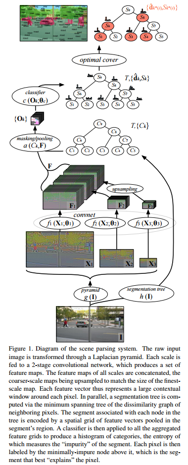
The full model is shown in the diagram below. It is an end-to-end trainable model for scene parsing.
Pre-processing
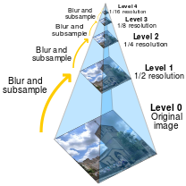
Before being put into the Convolutional Neural Network (CNN) multiple scaled versions of the image are generated. The set of these scaled images is called a pyramid. There were three different scale outputs of the image created, in a similar manner shown in the picture below
The scaling can be done by different transforms; the paper suggests to use the Laplacian transform. The Laplacian is the sum of partial second derivatives [math]\displaystyle{ \nabla^2 f = \frac{\partial^2 f}{\partial x^2} + \frac{\partial^2 f}{\partial y^2} }[/math]. A two-dimensional discrete approximation is given by the matrix [math]\displaystyle{ \left[\begin{array}{ccc}0 & 1 & 0 \\ 1 & -4 & 1 \\ 0 & 1 & 0\end{array}\right] }[/math].
Network Architecture
More holistic tasks, such as full-scene understanding (pixel-wise labeling, or any dense feature estimation) require the system to model complex interactions at the scale of complete images, not simply within a patch. In this problem the dimensionality becomes unmanageable: for a typical image of 256×256 pixels, a naive neural network would require millions of parameters, and a naive convolutional network would require filters that are unreasonably large to view enough context. The multiscale convolutional network overcomes these limitations by extending the concept of weight replication to the scale space. The more scales used to jointly train the models, the better the representation becomes for all scales. Using the same function to extract features at each scale is justified because the image content is scale invariant in principle. The authors noted that they observed worse performance when the weight sharing was removed.
Post-Processing
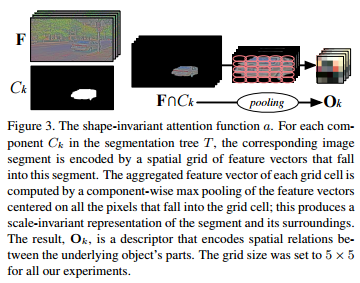
In this model the sampling is done using an elastic max-pooling function, which remaps input patterns of arbitrary size into a fixed G×G grid (in this case a 5x5 grid was used). This grid can be seen as a highly invariant representation that encodes spatial relations between an object’s attributes/parts. This representation is denoted Ok and is shown in the diagram below. With this encoding elongated or ill-shaped objects are nicely handled. The dominant features are also used to represent the object, and when combined with background subtraction, these features represent good basis functions to recognize the underlying object. These features are then associated to the corresponding areas of the tree segmentation of the image (generated by creating a minimum spanning tree from the dissimilarity graph of neighboring pixels) for optimal cover calculation.
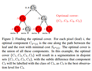
One of the important features of this model is its method for optimal cover, which is detailed in the diagram below. The leaf nodes represent pixels in the image and a subset of tree nodes are selected whose aggregate children span the entire image. The nodes are selected to minimize the average "impurity" of the class distribution (i.e. the entropy). The cover attempts to find an overall consisten segmentation, where each selected node corresponds to a particular class labelling for itself and all of its unselected children.
Training
Training is done in a two step process. First, the low level feature extractor [math]\displaystyle{ f_s }[/math] is trained to produce features that are maximally discriminative. Then, the classifier [math]\displaystyle{ c }[/math] is trained to predict the distriubiton of casses in a component. The feature vectors are obtained by concatenating the network outputs for different scales of the multiscale pyramid. To train for them the loss function [math]\displaystyle{ L_{\mathrm{cat}} = - \sum_{i \in \mathrm{pixels}, a \in \mathrm{classes}} c_{i,a} \ln(\hat{c}_{i,a}) }[/math] is used, where [math]\displaystyle{ c_i }[/math] is the true (classification) target vector and [math]\displaystyle{ \hat{c}_i }[/math] the prediction from a linear classifier (which is only used in this step and will be discarded later).
After training parameters for the feature extraction, parameters of the actual classifier is trained my minimizing the Kullback-Leibler-divergence (KL-divergence) between the true distribution of labels in each component and the prediction from the classifier. The KL-divergence is a measure of the difference between two probability distributions.
Experiments
For all experiments, a 2-stage convolutional network was used. The input is a 3-channel image, and it is transformed into a 16-dimensional feature map, using a bank of 16 7x7 filters followed by tanh units. This feature map is then pooled using a 2x2 max-pooling layer. The second layer transforms the 16-dimensional feature map into a 64-dimensional feature map, with each component being produced by a combination of 8 7x7 filters (for an effective total of 512 filters), followed by tanh units. This map is also pooled using a 2x2 max-pooling layer. This 64-dimensional feature map is transformed into a 256-dimensional feature map by using a combination of 16 7x7 filters (2048 filters).
The network is applied to a locally normalized Laplacian pyramid constructed on the input image. The pyramid contains three rescaled versions of the input: 320x240, 160x120, and 80x60. All of the inputs are properly padded and the outputs of each of the three networks are upsampled and concatenated to produce a 768-dimensional feature vector map (256x3). The network is trained on all three scales in parallel.
A simple grid search was used to find the best learning rate and regularization parameters (weight decay). A holdout of 10% of the training data was used as a validation set during the parameter search. For both datasets, jitter was used to artificially expand the size of the training data, to try to allow features to not overfit irrelevant biases present in the data. This jitter included horizontal flipping, and rotations between -8 and 8 degrees.
The hierarchy used to find the optimal cover is a constructed on the raw image gradient, based on a standard volume criterion<ref> F. Meyer and L. Najman. "Segmentation, minimum spanning tree and hierarchies." In L. Najman and H. Talbot, editors, Mathematical Morphology: from theory to application, chapter 9, pages 229–261. ISTE-Wiley, London, 2010. </ref><ref> J. Cousty and L. Najman. "Incremental algorithm for hierarchical minimum spanning forests and saliency of watershed cuts." In 10th International Symposium on Mathematical Morphology (ISMM’11), LNCS, 2011. </ref>, completed by removing non-informative small components (less than 100 pixels). Traditionally segmentation methods use a partition of segments (i.e. finding an optimal cut in the tree) rather than a cover. A number of graph cut methods were tried, but the results were systematically worse than the optimal cover method.
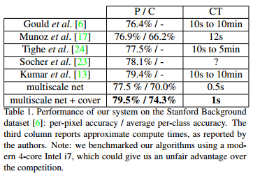
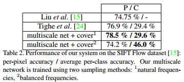
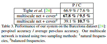
Two sampling methods for learning the multiscale features were tried on each dataset. One uses the natural frequencies of each class in the dataset, while the other balances them so that an equal number of each class is shown to the network. The results from each of these methods varied with the dataset used and are reported in the tables below. The authors only included the results for the frequency balancing method for the Stanford Background dataset as it consistently gave better results, but it could still be useful to have the results from the other method to help guide future work. Training with balanced frequencies allows better discrimination of small objects, and although it tends to have lower overall pixel-wise accuracy, it performs better from a recognition point of view. This observation can be seen in the tables below. The per-pixel accuracy for frequency balancing in the Barcelona dataset is quite poor, which the authors attribute by the fact that the dataset has a large amount of classes with very few training examples, leading to overfitting when trying to model them in this manner.
Results
References
<references />
