meProp: Sparsified Back Propagation for Accelerated Deep Learning with Reduced Overfitting
Introduction
A simple and effective technique for learning in neural networks has been introduced. Forward computation has been computed as it is typically computed. However. in back-propagation step only the top k elements (in magnitude) are retained for the computation of model parameters. Since only a small subset of the weight matrix is modified so it leads to a linear reduction in the computational cost. The results of the experiments suggest that accuracy is improved rather than being degraded. The name given to the proposed technique is minimal effort back propagation method (meProp).
In the process of neural network training, back propagation step entails the high computational cost because for each iteration it needs to compute full gradients and update all model parameters. The main idea of the paper is to find only the most critical and small subset of the gradient information and in each learning step update only this minimal subset of the parameters. This leads to sparsified gradients because only highly relevant parameters are updated and rest remain untouched.
Two important questions:
1) In the process of stochastic learning how to find that highly relevant subset of parameters from the current sample.
Solution to this question is given by Top-k search method to identify the most imp. parameters. After experiments with this solution the results demonstrate that we only update 1–4% of the weights at each back propagation pass which does not result in a larger number of training iterations.
2) Whether this selection of small subset of model parameters hurt the accuracy?
The results demonstrate that rather than reduction, this sparsification actually improves the accuracy. The inferred reason is that it is probably because the minimal effort update does not modify weakly relevant para-meters in each update, which makes the overfitting less likely, similar to the dropout effect.
The authors demonstrate the proposed approach using deep learning approaches (like LSTM, MLP), optimization approaches (like Adam and Adagrad) and tasks like NLP and Image Recognition.
Related Work
Some of the notable related work to this paper are as follows:
In 1990, Tollenaere et al.[1] proposed SuperSAB: an adaptive acceleration strategy for error back propagation learning. They proved that it may converge orders of magnitude faster than the original back propagation algorithm, and is only slightly instable. In addition, the algorithm is very insensitive to the choice of parameter values, and has excellent scaling properties.
In 1993, Riedmilller et al.[2] and Braun proposed an algorithm called RPROP, to overcome the inherent disadvantages of pure gradient-descent, it performed a local adaptation of the weight-updates according to the behavior of the error function.
In 2014, Srivastava et al.[3] proposed dropout. Large networks are also slow to use, making it difficult to deal with overfitting by combining the predictions of many different large neural nets at test time. The key idea is to randomly drop units (along with their connections) from the neural network during training. This prevents units from co-adapting too much.
The work proposed by the authors of meProp method is quite different than the three related works discussed above.
In 2017, Shazeer et al.[4] presented a Sparsely-Gated Mixture-of-Experts layer (MoE), consisting of up to thousands of feed-forward sub-networks. A trainable gating network determines a sparse combination of these experts to use for each example. They used this approach for the machine translation task and concluded that it gave significantly better results. Their method is limited to a specific set of mixture of experts however, the meProp method does not have these sort of limitations.
Proposed Approach
The original back propagation computes the "full gradient" for the input vector and the weight matrix. However For me-Prop, back propagation computes an "approximate gradient" by keeping top-k values of the backward flowed gradient and masking the remaining values to 0.
Where to apply meProp: In the learning task Matrix to Matrix and Matrix to Vector multiplications consumes more than 90% time of back propagation. Places where we apply meProp: -we apply meProp only to the back propagation from the output of the multiplication to its inputs. -we apply meProp (meaning top-k sparsification) to every hidden layer . Because the sparsified gradient will again be dense from one layer to another. -k for the output layer could be different from the k of the hidden layers because of the difference in dimensionality of the output layers. Example: For example, there are 10 tags in the MNIST task, so the dimension of the output layer is 10, and we use an MLP with the hidden dimension of 500. Thus, the best k for the output layer could be different from that of the hidden layers.
Exception: For other element-wise operations (e.g., activation functions), the original back propagation procedure remains as it is, be-cause those operations are already fast enough compared with matrix-matrix or matrix-vector multiplication operations.
Choice of top-k algorithms: A variant (focusing on memory reuse) of min heap based top-k selection method is used. The time complexity is: O(n log k) and space complexity is O(k). This is done to save time on sorting the entire vector.
Inverse Autoregressive Flow
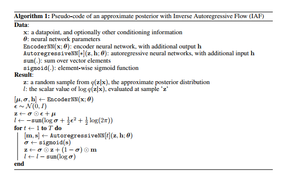
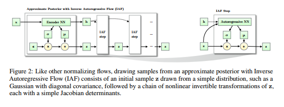
The answer presented by \cite{946paper} to the last question is \[ f_{k}(h_{k-1}) := \mu_{k} + \sigma_{k} \odot h_{k-1}, \] where $\odot$ means element-wise multiplication, $\mu_{k}$, $\sigma_{k}$ are outputs from an autoregressive neural network with inputs $h_{k-1}$ and an extra constant vector $c$ and we initialize with \[ h_{0} := \mu_{0} + \sigma_{0} \odot \epsilon \] such that $\epsilon \!\sim \mathcal{N}(0, I)$. The authors of \cite{946paper} call this series of functions the \textbf{inverse autoregressive flow}. We will solve the mystery of where this definition comes from later. The important point is that the functional form of $f_{k}$ is parametrized by the outputs of an autoregressive neural network and this implies that the Jacobians \[ \frac{\partial \mu_{k}}{\partial h_{k-1}}, \frac{\partial \sigma_{k}}{\partial h_{k-1}} \] are lower triangular with zeroes on the diagonal (this is not a trivial fact since $\mu_{k}$ and $\sigma_{k}$ are some complicated functions of $h_{k-1}$ -- they are outputs of a neural network which takes $h_{k-1}$ as an input). Hence, the derivative \[ \frac{\partial f_{k}}{\partial h_{k-1}} \] is a triangular matrix with the entries of $\sigma_{k}$ occupying the diagonal. The determinant of this is obviously just \[ \prod\limits^{D}_{i=1} \sigma_{k, i}, \] and it is very cheap to compute. Note also that the approximate posterior that comes out of this normalizing flow is \[ \log q_{K}(h_{K}) = - \sum\limits^{D}_{i=1} \left[ \frac{1}{2} \epsilon_{i}^{2} + \frac{1}{2} \log 2\pi + \sum\limits^{K}_{k=1} \log \sigma_{k,i} \right]. \] In conclusion, we have a nice expression for the ELBO. To round out the parsimony of the ELBO, we need an inference model which is computationally cheap to evaluate. Additionally, we typically do not calculate the ELBO gradients analytically but instead perform Monte Carlo estimation by sampling from the inference model. This requires inexpensive sampling from the inference model. Since expectations are calculated only with respect to the simple initial distribution $q_{0}$, both of these requirements are easily satisfied.
Inverse Autoregressive Transformations or, Whence Inverse Autoregressive Flow?
Once we have the inverse autoregressive flow, the main result of \cite{946paper} falls out. Let us consider how we could have come up with the idea of the inverse autoregressive flow. It will be helpful to start with a discussion of $\textbf{autoregressive neural networks}$, which we briefly alluded to when defining the flow. As the Latin prefix suggests, autoregression means that we deduce components of a random vector $h$ based on its \textit{own} components. More precisely, the $d^{th}$ element of $h$ depends on the preceding components $h_{1:d-1}$.
To elucidate this further, we shall follow the introductory exposition presented in \cite{MADE}. Let us consider a very simple autoencoder with just one hidden layer. That is, we have a feedforward neural network defined by \begin{align*} r(h) &:= g(b + Wh) \\ \hat{h} & := \mathrm{sigm}(c + Vr(h)), \end{align*} where $W$, $V$ are matrices of weights, $b$, $c$ are biases, $g$ is some non-linearity and $\mathrm{sigm}$ is element-wise sigmoid. Here, $r(h)$ is thought of as a hidden representation of the input $h$ and $\hat{h}$ is a reconstructed version of $h$. For simplicity, suppose that $h$ is a $D$-ary binary vector. Then we can measure the quality of our reconstruction using cross-entropy \[ l(h) := - \sum\limits h_{d} \log \hat{h}_{d} + (1 - h_{d}) \log (1 - \hat{h}_{d}). \] It is tempting to interpret $l(h)$ as a negative log-likelihood induced by the distribution \[ \prod\limits^{D}_{d=1} \hat{h}_{d}^{h_{d}} (1 - \hat{h}_{d})^{1 - h_{d}}. \] However, absent restrictions on the above expression, this is in general \textit{not} the case. As an example, suppose our hidden layer has as many units as the input layer. Then it is possible to drive the cross-entropy loss to $0$ by copying the input into the hidden layer. In this situation, $q(h) = 1$ for every possible $h$ and $q(h)$ is seen to actually not define a probability distribution.
If $l(h)$ is indeed to be a negative log-likelihood, i.e., \[ l(h) = - \log p(h) \] for a genuine probability distribution $p(h)$, it must satisfy \begin{align*} l(h) = & - \sum\limits^{D}_{d=1} \log p(h_{d} \mid h_{1:d-1}) \\ = & - \sum\limits^{D}_{d=1} h_{d} \log p(h_{d} = 1 \mid h_{1:d-1}) + (1 - h_{d}) \log p(h_{d} = 0 \mid h_{1:d-1}) \\ = & - \sum\limits^{D}_{d=1} h_{d} \log p(h_{d} = 1 \mid h_{1:d-1}) + (1 - h_{d})(1 - \log p(h_{d} = 1 \mid h_{1:d-1})). \end{align*} The first equation is just the chain rule of probability \[ p(h) = \prod\limits^{D}_{d=1} p(h_{d} \mid h_{1:d-1}), \] the second equation is true because of our assumption that each entry of $h$ is either $0$ or $1$ and the third equation holds due to the fact that $p(h)$ is a probability distribution. Comparing the naive cross-entropy loss \[ - \sum\limits h_{d} \log \hat{h}_{d} + (1 - h_{d}) \log (1 - \hat{h}_{d}) \] with the term \[ - \sum\limits^{D}_{d=1} h_{d} \log p(h_{d} = 1 \mid h_{1:d-1}) + (1 - h_{d})(1 - \log p(h_{d} = 1 \mid h_{1:d-1})), \] we see that a correct reconstruction (``correct" in the sense that the loss function is a negative log-likelihood) needs to satisfy \[ \hat{h}_{d} = \log p(h_{d} = 1 \mid h_{1:d-1}). \]
More generally, for a (deep) autoencoder we can require the reconstructed vector to have components satisfying \[ \hat{h}_{d} = p(h_{d} \mid h_{1:d-1}). \] In other words, the $d^{th}$ component is the probability of observing $h_{d}$ given the preceding components $h_{1:d-1}$. This latter property is known as the $\textbf{autoregressive property}$ since we can think of it as sequentially performing regression on the components of $h$. Unsurprisingly, an autoencoder satisfying the autoregressive property is called an $\textbf{autoregressive autoencoder}$.
Suppose now that we have an autoregressive autoencoder which takes an input vector $\mathbf{y} \in \mathbb{R}^{D}$ and we interpret the outputs of this network as parameters for a normal distribution. Write $[\mathbf{\mu}(\mathbf{y}),\mathbf{\sigma}(\mathbf{y})]$ for such output. The autoregressive structure implies that, for $j \in \{1, \ldots, D\}$, $\mathbf{y}_{j}$ depends only on the components $\mathbf{y}_{1:j-1}$. Therefore, if we take the vector $[\mathbf{\mu}_{i}, \mathbf{\sigma}_{i}]$ and compute the derivative with respect to $\mathbf{y}$, we will obtain a lower triangular matrix since \[ \frac{\partial [\mathbf{\mu}_{i}, \mathbf{\sigma}_{i}]}{\partial \mathbf{y}_{j}} = [0, 0] \] whenever $j \geq i$. We interpret the vector $[\mathbf{\mu}_{i}(\mathbf{y}_{1:j-1}), \mathbf{\sigma}_{i}(\mathbf{y}_{1:j-1})]$ as being the predicted mean and standard deviation of the $i^{th}$ element of (the reconstruction of) $\mathbf{y}$. In slightly more detail, the components of $\mathbf{y}$ are successively generated via \begin{align*} & \mathbf{y}_{0} = \mathbf{\mu}_{0} + \mathbf{\sigma}_{0} \cdot \mathbf{\epsilon}_{0}, \\ & \mathbf{y}_{i} = \mathbf{\mu}_{i}(\mathbf{y}_{1:i-1}) + \mathbf{\sigma}_{i}(\mathbf{y}_{1:i-1}) \cdot \mathbf{\epsilon}_{i}, \end{align*} where $\mathbf{\epsilon} \!\sim \mathcal{N}(\mathbf{0}, \mathbf{I})$.
To relate this back to the normalizing flow chosen by the authors of \cite{946paper}, replace $\mathbf{y}$ with $h_{k}$ as input to the autoregressive autoencoder and replace the outputs $\mathbf{\mu}$, $\mathbf{\sigma}$ with $\mu_{k}$, $\sigma_{k}$.
Implementation
The authors have open sourced the code for this paper on Github : https://github.com/openai/iaf
Experiments
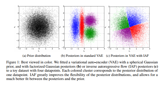
The authors showcase the potential for improvement of variational autoencoders afforded by the novel IAF methodology they proposed by providing empirical evidence in the context of two key benchmark datasets: MNIST and CIFAR 10.
MNIST DATASET:
The results of the experiment authors conducted are displayed in the figure below. 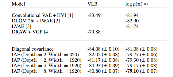
They provide some evidence as to the improvement of the variational inference via IAF when compared with other state of the art techniques.
CIFAR 10:
The results for the CIFAR 10 data set is displayed in the figure below. 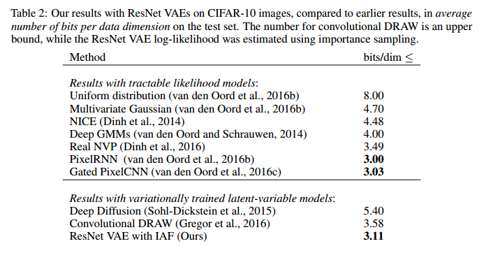
Concluding Remarks
In wrapping up, we note that there is something interesting about how the normalizing flow is derived. Essentially, the authors of \cite{946paper} took a neural network model with nice properties (fast sampling, simple Jacobian, etc.), looked at the function it implemented and basically dropped in this function in the recursive definition of the normalizing flow. This is not an isolated case. The authors of \cite{normalizing_flow} do much the same thing in coming up with the flow \[ f_{k}(h_{k}) = h_{k} + u_{k}s(w_{k}^{T}h_{k} + b_{k}). \] We believe that this flow is implicitly justified by the fact that functions of the above form are implemented by deep latent Gaussian models (see \cite{autoencoderRezende}). These flows, while interesting and useful, probably do not exhaust the possibilities for tractable and practical normalizing flows. It may be an interesting project to try and come up with novel normalizing flows by taking a favorite neural network architecture and using the function implemented by it as a flow. Additionally, it may be worth exploring boutique normalizing flows to improve variational inference in domain-specific settings (e.g., use a normalizing flow induced by a parsimonious convolutional neural network architecture for training an image-processing model using variational inference).
List of Figures
References
Blei, David M., Alp Kucukelbir, and Jon D. McAuliffe. "Variational inference: A review for statisticians." Journal of the American Statistical Association just-accepted (2017).
