meProp: Sparsified Back Propagation for Accelerated Deep Learning with Reduced Overfitting: Difference between revisions
No edit summary |
|||
| (233 intermediate revisions by 23 users not shown) | |||
| Line 1: | Line 1: | ||
=Introduction= | |||
The backpropagation step in neural network training entails high computational cost since each iteration requires calculation of full gradient vectors and matrices and subsequent update of all model parameters. | |||
The main idea of the paper is to find only a small but critical subset of the gradient information and in each learning step, update only this minimal subset of the parameters. This leads to sparsified gradients because only highly relevant parameters are updated and rest remain untouched. | |||
[[File:20.png|right|650px]] | |||
A simple and effective technique for neural networks learning is introduced in the current paper. The main technique entails a modification to the vanilla backpropagation algorithm. The idea is that after a forward pass has been carried out in the usual fashion, we retain only a subset of the full gradient for computation of model parameters. More precisely, a simple quantization technique is employed to sparsify the gradient vectors, viz., the entries of the first gradient in a backpropagation step are set to zero unless they reach a specified size threshold. The rest of the gradients (the ones with respect to the weights and biases of the neural network) are computed using the chain rule in the typical way using the sparsified gradient obtained from the top layer. Since only a small subset of the weight matrix is modified, we obtain a linear reduction in the computational cost. The experimental results presented in the paper suggest that accuracy is improved rather than being degraded. The name given to the proposed technique is minimal effort back propagation method (meProp). | |||
Fig. 1 shows an abstract view of the proposed approach. | |||
'''Two important questions:''' | |||
1) In the process of stochastic learning, how do we find a highly relevant subset of parameters from the current sample? | |||
One solution to this question is given by Top-$k$ search method to identify the most important parameters. Experimental results suggest that if we use this technique, then we can only update 1–4% of the weights at each back propagation pass and this does not result in a larger number of training iterations. | |||
Another likely solution I can think of is the method in the paper: [http://papers.nips.cc/paper/6372-learning-the-number-of-neurons-in-deep-networks.pdf Learning the Number of Neurons in Deep Networks]. We can use the group sparsity regularizer to identify the neurons that have many nonzero parameters, which are considered highly relevant parameters. | |||
2) Does this process of selecting a small subset of model parameters hurt accuracy? | |||
The | The results demonstrate that rather than reduce, this sparsification actually improves the accuracy in most settings. | ||
This result, while somewhat surprising, is attributed to a dropout-like effect which works to prevent overfitting. Because the minimal effort update does not modify any parameters which are weakly relevant, it seems sensible that this would help avoid overfitting the data. | |||
The | The authors demonstrate the proposed approach using deep learning approaches (like LSTM, MLP), optimization approaches (like Adam and Adagrad) and tasks like NLP and Image Recognition. | ||
=Related Work= | |||
Some of the notable related work to this paper are as follows: | |||
In 1990, Tollenaere et al.[1] proposed SuperSAB: an adaptive acceleration strategy for error back propagation learning. It is an improvement on SAB (self-adapting back propogation) strategy [7]. SuperSAB avoids taking a step when a change of sign in the weight derivative is discovered. Instead, it decreases the step size until a safe step is discovered (one without a sign change of the weight). They proved that it may converge orders of magnitude faster than the original back propagation algorithm, and is only slightly unstable. In addition, the algorithm is very insensitive to the choice of parameter values and has excellent scaling properties. | |||
In 1993, Riedmilller et al.[2] and Braun proposed an algorithm called RPROP, to overcome the inherent disadvantages of pure gradient-descent, it performed a local adaptation of the weight-updates according to the behavior of the error function. To be more specific, the authors defined an individual update-value for each weight. When the update of a weight is too large (mathematically, the partial derivative of a weight changes its sign), such update-value of this weight will decrease. Otherwise, it'll increase. After the process of adapting update-values is finished, the weight-update process is carried out as follows: when the partial derivative of the error function with respect to a specific weight is positive, the original weight decreases by its corresponding update-value, otherwise it increases. | |||
In 2014, Srivastava et al.[3] proposed dropout. Large networks are also slow to use, making it difficult to deal with overfitting by combining the predictions of many different large neural nets at test time. The key idea is to randomly drop units (along with their connections) from the neural network during training. This prevents units from co-adapting too much. | |||
The work proposed by the authors of meProp method is quite different from the three related works discussed above. | |||
In 2017, Shazeer et al.[4] presented a Sparsely-Gated Mixture-of-Experts layer (MoE), consisting of up to thousands of feed-forward sub-networks. A trainable gating network determines a sparse combination of these experts to use for each example. They used this approach for the machine translation task and concluded that it gave significantly better results. Their method is limited to a specific set of a mixture of experts however, the meProp method does not have these sort of limitations. | |||
=Proposed Approach= | |||
[[File:7.png|center|600px]] | |||
The original back propagation computes the "full gradient" for the input vector and the weight matrix. However, in me-Prop, back propagation computes an "approximate gradient" by keeping top-k values of the backward flowed gradient and masking the remaining values to 0. That is, only the top-k elements with the largest absolute values are kept and rest are made 0. | |||
Authors describe conversion of the traditional back-propagation to the back-propagation used in meProp with a computation unit with one linear transformation and one non-linear transformation as an example as given by eq. (1) and (2): | |||
\begin{align*} | \begin{align*} | ||
y &= W x \quad \quad \quad (1) | |||
\end{align*} | |||
\end{align*} | |||
\begin{align*} | \begin{align*} | ||
z &= \sigma (y) \quad \quad \quad (2) | |||
\end{align*} | \end{align*} | ||
where $W \in R_{n \times m}$, $x \in R_m$, $y \in R_n$, $z \in R_n$, $m$ is the dimension of the input vector, $n$ is the dimension of the output vector, and $\sigma$ is a non-linear function (e.g., ReLU, tanh, | |||
and sigmoid). During back propagation, we need to compute the gradient of the parameter matrix $W$ and the input vector $x$: | |||
\[ | \[ | ||
\frac{\partial z}{\partial W_{ij}} = \sigma^{'}_{i}x^{T}_{j},\quad i \quad \epsilon \quad [1,n], \quad j \quad \epsilon \quad [1,m] \quad \quad \quad (3) | |||
\] | \] | ||
\[ | \[ | ||
\frac{\partial z}{\partial x_{i}} = \sum\limits_j W^{T}_{ij} \sigma^{'}_{j},\quad i \quad \epsilon \quad [1,n], \quad j \quad \epsilon \quad [1,m] \quad \quad \quad (4) | |||
\] | \] | ||
Since the proposed meProp keeps only top-k elements based on the magnitude values so eq. (3) and (4) get transformed to (5) and (6), respectively: | |||
\[ | \[ | ||
\frac{\partial \ | \frac{\partial z}{\partial W_{ij}} \leftarrow \sigma^{'}_{i}x^{T}_{j}, \quad if \quad i \quad \epsilon \quad \{ t_{1}, t_{2},....., t_{k} \} \quad else \quad 0 \quad \quad (5) | ||
\] | \] | ||
\[ | \[ | ||
\frac{\partial | \frac{\partial z}{\partial x_{i}} \leftarrow \sum\limits_j W^{T}_{ij} \sigma^{'}_{j}, \quad if \quad j \quad \epsilon \quad \{ t_{1}, t_{2},....., t_{k} \} \quad else \quad 0 \quad \quad (6) | ||
\] | \] | ||
The original back-propagation computes the gradient of the matrix W and the gradient of the input vector x as shown in eq. (7) and (8), respectively: | |||
\[ | \[ | ||
\ | \frac{\partial L}{\partial W} = \frac{\partial L}{\partial y} . \frac{\partial y}{\partial W} \quad \quad (7) | ||
\] | \] | ||
\[ | \[ | ||
\ | \frac{\partial L}{\partial x} = \frac{\partial y}{\partial x} . \frac{\partial L}{\partial y} \quad \quad (8) | ||
\] | \] | ||
Since, the proposed meProp selects top-k elements of the traditional gradient to approximate it, hence the gradient of loss function with respect to W and x transform to the one shown in eq. (9) and (10): | |||
\[ | \[ | ||
\frac{\partial L}{\partial W} \leftarrow top_{k}(\frac{\partial L}{\partial y}) . \frac{\partial y}{\partial W} \quad \quad (9) | |||
\] | \] | ||
\[ | \[ | ||
\ | \frac{\partial L}{\partial x} \leftarrow \frac{\partial y}{\partial x} . top_{k}(\frac{\partial L}{\partial y}) \quad \quad (10) | ||
\] | \] | ||
The intuition behind the discussed conversions is depicted in Fig. 2. | |||
'''Where to apply meProp:''' | |||
In general, the authors leave the process of back propagation largely unchanged. Noting that, in the learning task Matrix-to-Matrix and Matrix-to-Vector multiplications consume more than 90% of the computation time, meProp is designed to improve the efficiencies there. The authors apply meProp only to the back propagation from the output of the multiplication to its inputs. Any operation which is applied elementwise (i.e. non-linear activation), the original back propagation algorithm remains unchanged. This means that for every hidden layer meProp is applied since between each hidden layer the gradient will remain dense. | |||
The authors note that the choice of $k$ could, and likely should, vary between the hidden layers and the output. Intuitively, if a network outputs with dimensionality 10, (say MNIST), and has a hidden layer with 500 nodes, taking $k$ close to 10 may be reasonable for the output, but is likely too small for the hidden layer. Despite this, the authors note that $k$ was kept constant for the paper. | |||
'''Choice of top-k algorithms:''' A variant (focusing on memory reuse) of min heap-based top-k selection method is used. The time complexity is: O(n log k) and space complexity is O(k). This is done to save time on sorting the entire vector. A min-heap is a binary tree such that the data contained in each node is less than (or equal to) the data in that node’s children. | |||
=Experiments and Configurations= | |||
To establish that the approach is general purpose, authors performed experiments on different deep learning algorithms(i.e. LSTM, MLP) with different optimizers (i.e. Adam, Adagrad) and different problem sets (i.e. Part of Speech Tagging, Transition based dependency parsing, MNIST Image Recognition). | |||
'''POS-Tag:''' | |||
Part-of-speech tagging is the process of identifying and assigning the parts of speech such as noun, verb, adjectice etc. in a corpus | |||
Baseline model: LSTM. Benchmark dataset: Penn Treebank Corpus. For training and testing: Wall Street Journal. | |||
'''Parsing:''' Baseline model: MLP. Benchmark dataset: Penn Treebank Corpus. For training, development, and testing: Wall Street Journal. The most common method for evaluating parsers are labeled and unlabeled attachment scores. In this work, the authors use the unlabeled attachment score. Labeled attachment refers to the correct matching of a word to its head along with the correct dependency relation. Unlabeled attachment ignores the dependency relation and focuses on the correctness of the assigned head. | |||
'''MNIST:''' | |||
The MNIST dataset consists of hand-written digits and the solution involves classifying the images among 10 digit classes. | |||
Baseline model: MLP. For training, development, and testing: MNIST dataset. | |||
In the configuration for Parsing and MNIST authors use the same k for the output and hidden layers. For POS-Tag authors use different k for the output and hidden layers. Due to low dimensionality of output layer in POS-Tag meProp isn't applied to it. | |||
The code for the paper can be found on Github : https://github.com/jklj077/meProp | |||
== | =Results= | ||
[[File:13.png|right|750px]] | |||
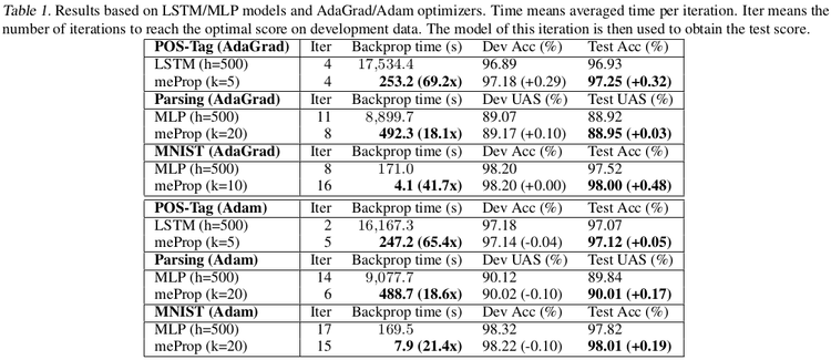
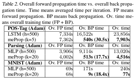
meProp is applied to the linear transformations which actually entail the major computational cost. Authors call linear transformation related backprop time as Backprop Time. It does not include the time required for non-linear activations which usually entail less than 2% of the computational cost. The total time of back propagation including non-linear activations is reported as Overall Backprop Time. | |||
Through results, it was observed that meProp substantially speeds up the backpropagation and provides a linear reduction in computational cost. Authors state the main reason for this reduction to be that meProp does not modify weakly relevant parameters, which makes overfitting less likely similar to the dropout effect. Also, the results depict that the proposed approach is independent of specific optimization methods. | |||
The graphs shown in Fig. 4 depict that meProp addresses the problem of overfitting and it provides better accuracy if the top-k weights are selected instead of random weights. The term backprop ratio in the figure is the ratio of k to the total number of parameters. It suggests that top-k elements contain | |||
the most important information of the gradients. This makes us think, instead of using dropout which randomly turns off few neurons, can it be done more deterministically based on the contribution of a neuron to the final prediction or output. Also, it was inferred that meProp can achieve further improvements over dropout for reducing overfitting and a model should take advantage of both meProp and dropout to reduce overfitting. Adding hidden layers does not hurt the performance of the model. Although this may be the case for the current set of test cases, a better understanding of the variation of hidden layer size and choice-of-k can be obtained by varying k with different hidden unit sizes <math>h</math> by keeping <math>k*h</math> or a similarly related term constant. This is better studied in [5] where the authors kept <math>p*n</math> constant to obtain greater reductions in training error for smaller p values ( p being the dropout coefficient. Low p, more units dropped). The relevant numerical results have been shown in table 1-5. | |||
''' | '''Further speed up:''' | ||
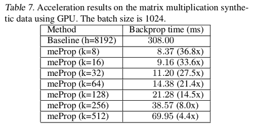
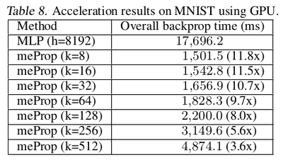
For further speeding up the backpropagation on GPUs authors presented a simple unified top-k approach (implementation in PyTorch). The main idea is to treat the entire mini-batch as a "big training example" where the top-k operation is based on the averaged values of all examples in the mini-batch so that the large consistent sparse matrix of the mini-batch can be converted into a dense small matrix by simply removing the zero values. The authors refer to this method as the simplified unified top-$k$ method. The results are presented in Table 6. This GPU acceleration works much more outstandingly for heavy models, with the relevant numerical results shown in table 7 and 8. | |||
=List of Tables= | |||
[[File:11.png|thumb|center|750px]] | |||
[[File:12.png|thumb|center|450px]] | |||
[[File:14.png|thumb|center|350px]] | |||
[[File:15.png|thumb|center|400px]] | |||
[[File:16.png|thumb|center|500px]] | |||
[[File:meProp.PNG|thumb|center|750px]] | |||
[[File:56.png|thumb|center|500px]] | |||
[[File:57.png|thumb|center|400px]] | |||
=Critiques= | |||
The main idea behind meProp is to wipe out the backprop mechanism of (n-k) nodes where "n" is the number of nodes in the current layer and "k" is the number of nodes contributing to the maximum of the loss in that layer. Intuitively, meProp in backpropagation process is actually a threshold w.r.t. k, or an activation function in the gradient backpropagation: only if the gradients are big enough in magnitude that will be passed to the previous layer. Referring to equation 10, | |||
\[ | \[ | ||
\frac{\partial L}{\partial x} \leftarrow \frac{\partial y}{\partial x} . top_{k}(\frac{\partial L}{\partial y}) \quad \quad | |||
\] | \] | ||
#The authors have not proposed any method on how k should be selected, hence it is left to the reader's discretion to possibly take it as a hyperparameter. If so, in a deeply layered architecture, where the weights between each layer are randomly initialized during each execution, "k" might change for each layer since the features learned at each layer may not be the same from the previous layers. However, under the assumption that we only perform top-$k$ selection for the gradient vector associated to the top layer, we do not choose $k$ for each subsequent layer through which we backpropagate. The concern as to whether we may lose valuable feature selection due to hidden layers is a valuable one. Moreover, further study should be carried out to see whether this is, in fact, the case and if not, whether we can directly sparsify weight matrices of hidden layers. | |||
#If the sum of losses caused by the (n-k) nodes in the current layer exceed any of the losses incurred due to "k" nodes, then it would not be correct to drop the (n-k) nodes as we can assume the aggregate (n-k) nodes as a single opaque node with a composite weight which will incur an aggregated loss greater than any of the "k" nodes. | |||
In essence, the idea of selecting "k" nodes to drop-out prove to be effective as shown by the authors, but the lack of information on the conditions on selecting "k" for each layer given the current state of the layer might lead to lack of consistency in the results. | |||
In addition to this, the authors did not include convolutional neural networks in their experiments. It would have been interesting to see whether similar results were observed on that architecture. Theoretically, the method presented in this paper should only update kernels in parts of an image that contribute the most to the loss. | |||
As the experiment settings, all networks are using Adam and AdaGrad, it is an interesting guess that whether the choice of the optimizer will influence the accuracy. The authors did not include the results with SGD(momentum). Since Adam and AdaGrad are using adaptive learning rate for each weight. | |||
There has been no mention by the authors on the loss ( significant loss or the insignificance) of using meProp on tasks where preservation of temporal information and contextual data is important. For example, in tasks like using RNNs for Question-Answering tasks, the memory of details of earlier regions of the paragraph could be garbled due to not updating the weights which do not belong to the top-k set in backpropagation. Indeed, the lack of principled methods for sparsification is a major issue in this case since tasks such as machine translation often entail data where certain parts of an input are much more predictive than other parts in a systematic way. There could be a trade-off between knowledge preservation and choice of the hyperparameter k which can be verified by further analysis like correlation/covariance studies. | |||
The approach can be thought of as a deterministic Dropout giving priority to higher gradient contributing connections during backpropagation. However, unlike dropout (which is random in nature), selecting k-top may permanently exclude some parts of NN from training at all, which has not been mentioned in the paper at all. Authors have also failed to test their approach on bigger datasets such as Imagenet, therefore it might be possible that dataset (MNIST) used by the authors is too simple for the given NN architecture, therefore, meProp approach helped to generalize the model better. It is generally a bad habit to use MNIST results in 2017's research works, as they shed no light on the real world AI problems. The idea is really simple, basically applying only k strongest gradients during backprop which should work for different architectures as well (LSTM, RNNs). This paper has shown the advantage of their method empirically, but only in a simple dataset.It is lacking its results in a real world and more complex dataset. Lastly, the approximate gradient introduced here can be interpreted as a projection of the actual gradient on some lower dimensional subspace. This observation suggests that this method might have some connections with the projected gradient optimization algorithm. | |||
=References= | |||
# Tollenaere, Tom. "SuperSAB: fast adaptive back propagation with good scaling properties." Neural networks 3.5 (1990): 561-573. | |||
# Riedmiller, Martin, and Heinrich Braun. "A direct adaptive method for faster backpropagation learning: The RPROP algorithm." Neural Networks, 1993., IEEE International Conference on. IEEE, 1993. | |||
# Srivastava, Nitish, et al. "Dropout: a simple way to prevent neural networks from overfitting." Journal of machine learning research 15.1 (2014): 1929-1958. | |||
# Shazeer, Noam, et al. "Outrageously large neural networks: The sparsely-gated mixture-of-experts layer." arXiv preprint arXiv:1701.06538 (2017). | |||
# Nitish Srivastava, Geoffrey Hinton, Alex Krizhevsky, Ilya Sutskever, Ruslan Salakhutdinov. "Dropout: A Simple Way to Prevent Neural Networks from Overfitting", Journal of Machine Learning Research 15 (2014) 1929-1958 | |||
# Speech and Language Processing. Daniel Jurafsky & James H. Martin. 2017. Draft of August 28, 2017. | |||
# Devos. M. R., Orban. G. A. "Self adaptive backpropagation." Proceedings NeuroNimes 1988. | |||
Latest revision as of 20:40, 28 November 2017
Introduction
The backpropagation step in neural network training entails high computational cost since each iteration requires calculation of full gradient vectors and matrices and subsequent update of all model parameters. The main idea of the paper is to find only a small but critical subset of the gradient information and in each learning step, update only this minimal subset of the parameters. This leads to sparsified gradients because only highly relevant parameters are updated and rest remain untouched.
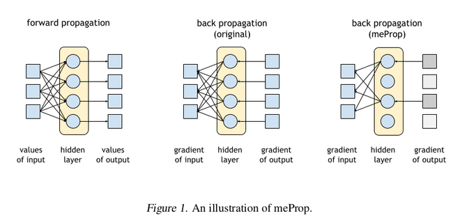
A simple and effective technique for neural networks learning is introduced in the current paper. The main technique entails a modification to the vanilla backpropagation algorithm. The idea is that after a forward pass has been carried out in the usual fashion, we retain only a subset of the full gradient for computation of model parameters. More precisely, a simple quantization technique is employed to sparsify the gradient vectors, viz., the entries of the first gradient in a backpropagation step are set to zero unless they reach a specified size threshold. The rest of the gradients (the ones with respect to the weights and biases of the neural network) are computed using the chain rule in the typical way using the sparsified gradient obtained from the top layer. Since only a small subset of the weight matrix is modified, we obtain a linear reduction in the computational cost. The experimental results presented in the paper suggest that accuracy is improved rather than being degraded. The name given to the proposed technique is minimal effort back propagation method (meProp).
Fig. 1 shows an abstract view of the proposed approach.
Two important questions:
1) In the process of stochastic learning, how do we find a highly relevant subset of parameters from the current sample?
One solution to this question is given by Top-$k$ search method to identify the most important parameters. Experimental results suggest that if we use this technique, then we can only update 1–4% of the weights at each back propagation pass and this does not result in a larger number of training iterations.
Another likely solution I can think of is the method in the paper: Learning the Number of Neurons in Deep Networks. We can use the group sparsity regularizer to identify the neurons that have many nonzero parameters, which are considered highly relevant parameters.
2) Does this process of selecting a small subset of model parameters hurt accuracy?
The results demonstrate that rather than reduce, this sparsification actually improves the accuracy in most settings. This result, while somewhat surprising, is attributed to a dropout-like effect which works to prevent overfitting. Because the minimal effort update does not modify any parameters which are weakly relevant, it seems sensible that this would help avoid overfitting the data.
The authors demonstrate the proposed approach using deep learning approaches (like LSTM, MLP), optimization approaches (like Adam and Adagrad) and tasks like NLP and Image Recognition.
Related Work
Some of the notable related work to this paper are as follows:
In 1990, Tollenaere et al.[1] proposed SuperSAB: an adaptive acceleration strategy for error back propagation learning. It is an improvement on SAB (self-adapting back propogation) strategy [7]. SuperSAB avoids taking a step when a change of sign in the weight derivative is discovered. Instead, it decreases the step size until a safe step is discovered (one without a sign change of the weight). They proved that it may converge orders of magnitude faster than the original back propagation algorithm, and is only slightly unstable. In addition, the algorithm is very insensitive to the choice of parameter values and has excellent scaling properties.
In 1993, Riedmilller et al.[2] and Braun proposed an algorithm called RPROP, to overcome the inherent disadvantages of pure gradient-descent, it performed a local adaptation of the weight-updates according to the behavior of the error function. To be more specific, the authors defined an individual update-value for each weight. When the update of a weight is too large (mathematically, the partial derivative of a weight changes its sign), such update-value of this weight will decrease. Otherwise, it'll increase. After the process of adapting update-values is finished, the weight-update process is carried out as follows: when the partial derivative of the error function with respect to a specific weight is positive, the original weight decreases by its corresponding update-value, otherwise it increases.
In 2014, Srivastava et al.[3] proposed dropout. Large networks are also slow to use, making it difficult to deal with overfitting by combining the predictions of many different large neural nets at test time. The key idea is to randomly drop units (along with their connections) from the neural network during training. This prevents units from co-adapting too much.
The work proposed by the authors of meProp method is quite different from the three related works discussed above.
In 2017, Shazeer et al.[4] presented a Sparsely-Gated Mixture-of-Experts layer (MoE), consisting of up to thousands of feed-forward sub-networks. A trainable gating network determines a sparse combination of these experts to use for each example. They used this approach for the machine translation task and concluded that it gave significantly better results. Their method is limited to a specific set of a mixture of experts however, the meProp method does not have these sort of limitations.
Proposed Approach
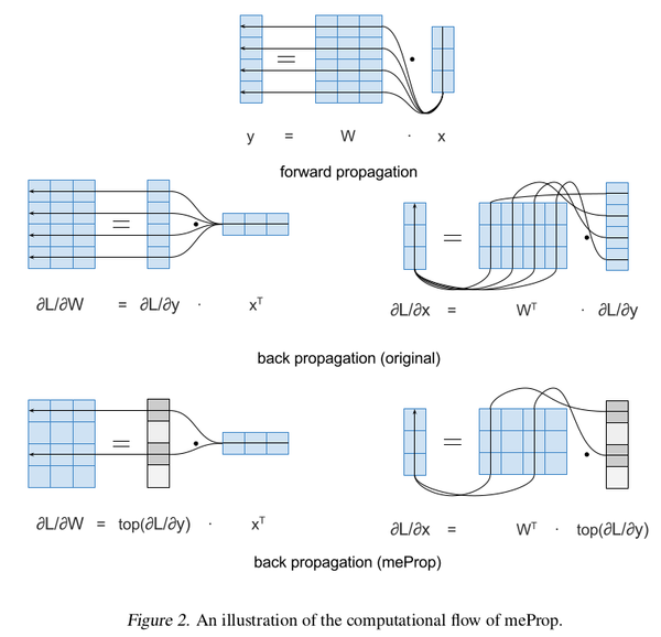
The original back propagation computes the "full gradient" for the input vector and the weight matrix. However, in me-Prop, back propagation computes an "approximate gradient" by keeping top-k values of the backward flowed gradient and masking the remaining values to 0. That is, only the top-k elements with the largest absolute values are kept and rest are made 0.
Authors describe conversion of the traditional back-propagation to the back-propagation used in meProp with a computation unit with one linear transformation and one non-linear transformation as an example as given by eq. (1) and (2): \begin{align*} y &= W x \quad \quad \quad (1) \end{align*} \begin{align*} z &= \sigma (y) \quad \quad \quad (2) \end{align*} where $W \in R_{n \times m}$, $x \in R_m$, $y \in R_n$, $z \in R_n$, $m$ is the dimension of the input vector, $n$ is the dimension of the output vector, and $\sigma$ is a non-linear function (e.g., ReLU, tanh, and sigmoid). During back propagation, we need to compute the gradient of the parameter matrix $W$ and the input vector $x$:
\[ \frac{\partial z}{\partial W_{ij}} = \sigma^{'}_{i}x^{T}_{j},\quad i \quad \epsilon \quad [1,n], \quad j \quad \epsilon \quad [1,m] \quad \quad \quad (3) \]
\[ \frac{\partial z}{\partial x_{i}} = \sum\limits_j W^{T}_{ij} \sigma^{'}_{j},\quad i \quad \epsilon \quad [1,n], \quad j \quad \epsilon \quad [1,m] \quad \quad \quad (4) \]
Since the proposed meProp keeps only top-k elements based on the magnitude values so eq. (3) and (4) get transformed to (5) and (6), respectively:
\[ \frac{\partial z}{\partial W_{ij}} \leftarrow \sigma^{'}_{i}x^{T}_{j}, \quad if \quad i \quad \epsilon \quad \{ t_{1}, t_{2},....., t_{k} \} \quad else \quad 0 \quad \quad (5) \]
\[ \frac{\partial z}{\partial x_{i}} \leftarrow \sum\limits_j W^{T}_{ij} \sigma^{'}_{j}, \quad if \quad j \quad \epsilon \quad \{ t_{1}, t_{2},....., t_{k} \} \quad else \quad 0 \quad \quad (6) \]
The original back-propagation computes the gradient of the matrix W and the gradient of the input vector x as shown in eq. (7) and (8), respectively:
\[ \frac{\partial L}{\partial W} = \frac{\partial L}{\partial y} . \frac{\partial y}{\partial W} \quad \quad (7) \]
\[ \frac{\partial L}{\partial x} = \frac{\partial y}{\partial x} . \frac{\partial L}{\partial y} \quad \quad (8) \]
Since, the proposed meProp selects top-k elements of the traditional gradient to approximate it, hence the gradient of loss function with respect to W and x transform to the one shown in eq. (9) and (10):
\[
\frac{\partial L}{\partial W} \leftarrow top_{k}(\frac{\partial L}{\partial y}) . \frac{\partial y}{\partial W} \quad \quad (9)
\]
\[ \frac{\partial L}{\partial x} \leftarrow \frac{\partial y}{\partial x} . top_{k}(\frac{\partial L}{\partial y}) \quad \quad (10) \]
The intuition behind the discussed conversions is depicted in Fig. 2.
Where to apply meProp: In general, the authors leave the process of back propagation largely unchanged. Noting that, in the learning task Matrix-to-Matrix and Matrix-to-Vector multiplications consume more than 90% of the computation time, meProp is designed to improve the efficiencies there. The authors apply meProp only to the back propagation from the output of the multiplication to its inputs. Any operation which is applied elementwise (i.e. non-linear activation), the original back propagation algorithm remains unchanged. This means that for every hidden layer meProp is applied since between each hidden layer the gradient will remain dense.
The authors note that the choice of $k$ could, and likely should, vary between the hidden layers and the output. Intuitively, if a network outputs with dimensionality 10, (say MNIST), and has a hidden layer with 500 nodes, taking $k$ close to 10 may be reasonable for the output, but is likely too small for the hidden layer. Despite this, the authors note that $k$ was kept constant for the paper.
Choice of top-k algorithms: A variant (focusing on memory reuse) of min heap-based top-k selection method is used. The time complexity is: O(n log k) and space complexity is O(k). This is done to save time on sorting the entire vector. A min-heap is a binary tree such that the data contained in each node is less than (or equal to) the data in that node’s children.
Experiments and Configurations
To establish that the approach is general purpose, authors performed experiments on different deep learning algorithms(i.e. LSTM, MLP) with different optimizers (i.e. Adam, Adagrad) and different problem sets (i.e. Part of Speech Tagging, Transition based dependency parsing, MNIST Image Recognition).
POS-Tag: Part-of-speech tagging is the process of identifying and assigning the parts of speech such as noun, verb, adjectice etc. in a corpus Baseline model: LSTM. Benchmark dataset: Penn Treebank Corpus. For training and testing: Wall Street Journal.
Parsing: Baseline model: MLP. Benchmark dataset: Penn Treebank Corpus. For training, development, and testing: Wall Street Journal. The most common method for evaluating parsers are labeled and unlabeled attachment scores. In this work, the authors use the unlabeled attachment score. Labeled attachment refers to the correct matching of a word to its head along with the correct dependency relation. Unlabeled attachment ignores the dependency relation and focuses on the correctness of the assigned head.
MNIST: The MNIST dataset consists of hand-written digits and the solution involves classifying the images among 10 digit classes. Baseline model: MLP. For training, development, and testing: MNIST dataset.
In the configuration for Parsing and MNIST authors use the same k for the output and hidden layers. For POS-Tag authors use different k for the output and hidden layers. Due to low dimensionality of output layer in POS-Tag meProp isn't applied to it.
The code for the paper can be found on Github : https://github.com/jklj077/meProp
Results

meProp is applied to the linear transformations which actually entail the major computational cost. Authors call linear transformation related backprop time as Backprop Time. It does not include the time required for non-linear activations which usually entail less than 2% of the computational cost. The total time of back propagation including non-linear activations is reported as Overall Backprop Time.
Through results, it was observed that meProp substantially speeds up the backpropagation and provides a linear reduction in computational cost. Authors state the main reason for this reduction to be that meProp does not modify weakly relevant parameters, which makes overfitting less likely similar to the dropout effect. Also, the results depict that the proposed approach is independent of specific optimization methods.
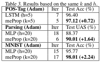
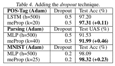
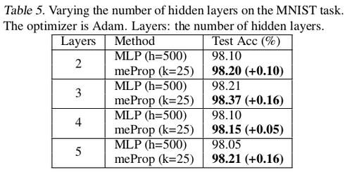
The graphs shown in Fig. 4 depict that meProp addresses the problem of overfitting and it provides better accuracy if the top-k weights are selected instead of random weights. The term backprop ratio in the figure is the ratio of k to the total number of parameters. It suggests that top-k elements contain the most important information of the gradients. This makes us think, instead of using dropout which randomly turns off few neurons, can it be done more deterministically based on the contribution of a neuron to the final prediction or output. Also, it was inferred that meProp can achieve further improvements over dropout for reducing overfitting and a model should take advantage of both meProp and dropout to reduce overfitting. Adding hidden layers does not hurt the performance of the model. Although this may be the case for the current set of test cases, a better understanding of the variation of hidden layer size and choice-of-k can be obtained by varying k with different hidden unit sizes [math]\displaystyle{ h }[/math] by keeping [math]\displaystyle{ k*h }[/math] or a similarly related term constant. This is better studied in [5] where the authors kept [math]\displaystyle{ p*n }[/math] constant to obtain greater reductions in training error for smaller p values ( p being the dropout coefficient. Low p, more units dropped). The relevant numerical results have been shown in table 1-5.
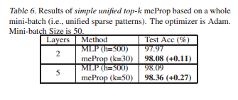
Further speed up: For further speeding up the backpropagation on GPUs authors presented a simple unified top-k approach (implementation in PyTorch). The main idea is to treat the entire mini-batch as a "big training example" where the top-k operation is based on the averaged values of all examples in the mini-batch so that the large consistent sparse matrix of the mini-batch can be converted into a dense small matrix by simply removing the zero values. The authors refer to this method as the simplified unified top-$k$ method. The results are presented in Table 6. This GPU acceleration works much more outstandingly for heavy models, with the relevant numerical results shown in table 7 and 8.
List of Tables
Critiques
The main idea behind meProp is to wipe out the backprop mechanism of (n-k) nodes where "n" is the number of nodes in the current layer and "k" is the number of nodes contributing to the maximum of the loss in that layer. Intuitively, meProp in backpropagation process is actually a threshold w.r.t. k, or an activation function in the gradient backpropagation: only if the gradients are big enough in magnitude that will be passed to the previous layer. Referring to equation 10, \[ \frac{\partial L}{\partial x} \leftarrow \frac{\partial y}{\partial x} . top_{k}(\frac{\partial L}{\partial y}) \quad \quad \]
- The authors have not proposed any method on how k should be selected, hence it is left to the reader's discretion to possibly take it as a hyperparameter. If so, in a deeply layered architecture, where the weights between each layer are randomly initialized during each execution, "k" might change for each layer since the features learned at each layer may not be the same from the previous layers. However, under the assumption that we only perform top-$k$ selection for the gradient vector associated to the top layer, we do not choose $k$ for each subsequent layer through which we backpropagate. The concern as to whether we may lose valuable feature selection due to hidden layers is a valuable one. Moreover, further study should be carried out to see whether this is, in fact, the case and if not, whether we can directly sparsify weight matrices of hidden layers.
- If the sum of losses caused by the (n-k) nodes in the current layer exceed any of the losses incurred due to "k" nodes, then it would not be correct to drop the (n-k) nodes as we can assume the aggregate (n-k) nodes as a single opaque node with a composite weight which will incur an aggregated loss greater than any of the "k" nodes.
In essence, the idea of selecting "k" nodes to drop-out prove to be effective as shown by the authors, but the lack of information on the conditions on selecting "k" for each layer given the current state of the layer might lead to lack of consistency in the results.
In addition to this, the authors did not include convolutional neural networks in their experiments. It would have been interesting to see whether similar results were observed on that architecture. Theoretically, the method presented in this paper should only update kernels in parts of an image that contribute the most to the loss.
As the experiment settings, all networks are using Adam and AdaGrad, it is an interesting guess that whether the choice of the optimizer will influence the accuracy. The authors did not include the results with SGD(momentum). Since Adam and AdaGrad are using adaptive learning rate for each weight.
There has been no mention by the authors on the loss ( significant loss or the insignificance) of using meProp on tasks where preservation of temporal information and contextual data is important. For example, in tasks like using RNNs for Question-Answering tasks, the memory of details of earlier regions of the paragraph could be garbled due to not updating the weights which do not belong to the top-k set in backpropagation. Indeed, the lack of principled methods for sparsification is a major issue in this case since tasks such as machine translation often entail data where certain parts of an input are much more predictive than other parts in a systematic way. There could be a trade-off between knowledge preservation and choice of the hyperparameter k which can be verified by further analysis like correlation/covariance studies.
The approach can be thought of as a deterministic Dropout giving priority to higher gradient contributing connections during backpropagation. However, unlike dropout (which is random in nature), selecting k-top may permanently exclude some parts of NN from training at all, which has not been mentioned in the paper at all. Authors have also failed to test their approach on bigger datasets such as Imagenet, therefore it might be possible that dataset (MNIST) used by the authors is too simple for the given NN architecture, therefore, meProp approach helped to generalize the model better. It is generally a bad habit to use MNIST results in 2017's research works, as they shed no light on the real world AI problems. The idea is really simple, basically applying only k strongest gradients during backprop which should work for different architectures as well (LSTM, RNNs). This paper has shown the advantage of their method empirically, but only in a simple dataset.It is lacking its results in a real world and more complex dataset. Lastly, the approximate gradient introduced here can be interpreted as a projection of the actual gradient on some lower dimensional subspace. This observation suggests that this method might have some connections with the projected gradient optimization algorithm.
References
- Tollenaere, Tom. "SuperSAB: fast adaptive back propagation with good scaling properties." Neural networks 3.5 (1990): 561-573.
- Riedmiller, Martin, and Heinrich Braun. "A direct adaptive method for faster backpropagation learning: The RPROP algorithm." Neural Networks, 1993., IEEE International Conference on. IEEE, 1993.
- Srivastava, Nitish, et al. "Dropout: a simple way to prevent neural networks from overfitting." Journal of machine learning research 15.1 (2014): 1929-1958.
- Shazeer, Noam, et al. "Outrageously large neural networks: The sparsely-gated mixture-of-experts layer." arXiv preprint arXiv:1701.06538 (2017).
- Nitish Srivastava, Geoffrey Hinton, Alex Krizhevsky, Ilya Sutskever, Ruslan Salakhutdinov. "Dropout: A Simple Way to Prevent Neural Networks from Overfitting", Journal of Machine Learning Research 15 (2014) 1929-1958
- Speech and Language Processing. Daniel Jurafsky & James H. Martin. 2017. Draft of August 28, 2017.
- Devos. M. R., Orban. G. A. "Self adaptive backpropagation." Proceedings NeuroNimes 1988.