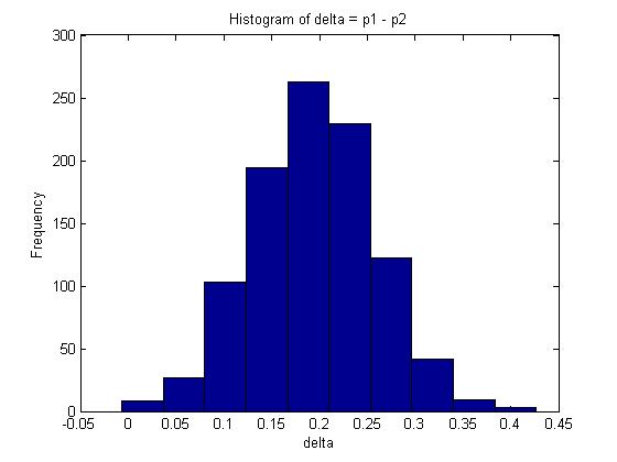
binomial Probability Monte Carlo Sampling June 2 2009

Example 1:

You are given two independent Binomial distributions with probabilities [math]\displaystyle{ \displaystyle p_1\text{, }p_2 }[/math]. Using a Monte Carlo simulation, approximate the value of [math]\displaystyle{ \displaystyle \delta }[/math], where [math]\displaystyle{ \displaystyle \delta = p_1 - p_2 }[/math].

[math]\displaystyle{ \displaystyle X \sim BIN(n, p_1) }[/math]; [math]\displaystyle{ \displaystyle Y \sim BIN(n, p_2) }[/math]; [math]\displaystyle{ \displaystyle \delta = p_1 - p_2 }[/math]

So [math]\displaystyle{ \displaystyle f(p_1, p_2 | x,y) = \frac{f(x, y|p_1, p_2)*f(p_1,p_2)}{f(x,y)} }[/math] where [math]\displaystyle{ \displaystyle f(x,y) }[/math] is a flat distribution and the expected value of [math]\displaystyle{ \displaystyle \delta }[/math] is as follows:

[math]\displaystyle{ \displaystyle \hat{\delta} = \int\int\delta f(p_1,p_2|X,Y)\,dp_1dp_2 }[/math]

Since X, Y are independent, we can split the conditional probability distribution:

[math]\displaystyle{ \displaystyle f(p_1,p_2|X,Y) \propto f(p_1|X)f(p_2|Y) }[/math]

We need to find conditional distribution functions for [math]\displaystyle{ \displaystyle p_1, p_2 }[/math] to draw samples from. In order to get a distribution for the probability 'p' of a Binomial, we have to divide the Binomial distribution by n. This new distribution has the same shape as the original, but is scaled. A Beta distribution is a suitable approximation. Let

[math]\displaystyle{ \displaystyle f(p_1 | X) \sim \text{Beta}(x+1, n-x+1) }[/math] and [math]\displaystyle{ \displaystyle f(p_2 | Y) \sim \text{Beta}(y+1, n-y+1) }[/math], where

[math]\displaystyle{ \displaystyle \text{Beta}(\alpha,\beta) = \frac{\Gamma(\alpha+\beta)}{\Gamma(\alpha)\Gamma(\beta)}p^{\alpha-1}(1-p)^{\beta-1} }[/math]

Process:

1. Draw samples for [math]\displaystyle{ \displaystyle p_1 }[/math] and [math]\displaystyle{ \displaystyle p_2 }[/math]: [math]\displaystyle{ \displaystyle (p_1,p_2)^{(1)} }[/math], [math]\displaystyle{ \displaystyle (p_1,p_2)^{(2)} }[/math], ..., [math]\displaystyle{ \displaystyle (p_1,p_2)^{(n)} }[/math];
2. Compute [math]\displaystyle{ \displaystyle \delta = p_1 - p_2 }[/math] in order to get n values for [math]\displaystyle{ \displaystyle \delta }[/math];
3. [math]\displaystyle{ \displaystyle \hat{\delta}=\frac{\displaystyle\sum_{\forall i}\delta^{(i)}}{N} }[/math].
   
   

Matlab Code:

The Matlab code for recreating the above example is as follows:

n=100; %number of trials for X
m=100; %number of trials for Y
x=80; %number of successes for X trials
y=60; %number of successes for y trials
p1=betarnd(x+1, n-x+1, 1, 1000);
p2=betarnd(y+1, m-y+1, 1, 1000);
delta=p1-p2;
mean(delta);

The mean in this example is given by 0.1938.

A 95% confidence interval for [math]\displaystyle{ \delta }[/math] is represented by the interval between the 2.5% and 97.5% quantiles which covers 95% of the probability distribution. In Matlab, this can be calculated as follows:

q1=quantile(delta,0.025);
q2=quantile(delta,0.975);

The interval is approximately [math]\displaystyle{ 95% CI \approx (0.06606, 0.32204) }[/math]

The histogram of delta is:

Note: In this case, we can also find [math]\displaystyle{ E(\delta) }[/math] analytically since [math]\displaystyle{ E(\delta) = E(p_1 - p_2) = E(p_1) - E(p_2) = \frac{x+1}{n+2} - \frac{y+1}{m+2} \approx 0.1961 }[/math]. Compare this with the maximum likelihood estimate for [math]\displaystyle{ \delta }[/math]: [math]\displaystyle{ \frac{x}{n} - \frac{y}{m} = 0.2 }[/math].

Example 2:

We conduct an experiment by giving rats one of ten possible doses of a drug, where each subsequent dose is more lethal than the previous one:

[math]\displaystyle{ \displaystyle x_1\lt x_2\lt ...\lt x_{10} }[/math]

For each dose [math]\displaystyle{ \displaystyle x_i }[/math] we test n rats and observe [math]\displaystyle{ \displaystyle Y_i }[/math], the number of rats that survive. Therefore,

[math]\displaystyle{ \displaystyle Y_i \sim~ BIN(n, p_i) }[/math]
.

We can assume that the probability of death grows with the concentration of drug given, i.e. [math]\displaystyle{ \displaystyle p_1\lt p_2\lt ...\lt p_{10} }[/math]. Estimate the dose at which the animals have at least 50% chance of dying.

Let [math]\displaystyle{ \displaystyle \delta=x_j }[/math] where [math]\displaystyle{ \displaystyle j=min\{i|p_i\geq0.5\} }[/math]

We are interested in [math]\displaystyle{ \displaystyle \delta }[/math] since any higher concentrations are known to have a higher death rate.

Solving this analytically is difficult:

[math]\displaystyle{ \displaystyle \delta = g(p_1, p_2, ..., p_{10}) }[/math] where g is an unknown function

[math]\displaystyle{ \displaystyle \hat{\delta} = \int \int..\int_A \delta f(p_1,p_2,...,p_{10}|Y_1,Y_2,...,Y_{10})\,dp_1dp_2...dp_{10} }[/math]

where [math]\displaystyle{ \displaystyle A=\{(p_1,p_2,...,p_{10})|p_1\leq p_2\leq ...\leq p_{10} \} }[/math]

Process: Monte Carlo
We assume that

1. Draw [math]\displaystyle{ \displaystyle p_i \sim~ BETA(y_i+1, n-y_i+1) }[/math]
2. Keep sample only if it satisfies [math]\displaystyle{ \displaystyle p_1\leq p_2\leq ...\leq p_{10} }[/math], otherwise discard and try again.
3. Compute [math]\displaystyle{ \displaystyle \delta }[/math] by finding the first [math]\displaystyle{ \displaystyle p_i }[/math] sample with over 50% deaths.
4. Repeat process n times to get n estimates for [math]\displaystyle{ \displaystyle \delta_1, \delta_2, ..., \delta_N }[/math].
5. [math]\displaystyle{ \displaystyle \bar{\delta} = \frac{\displaystyle\sum_{\forall i} \delta_i}{N} }[/math].