Zero-Shot Visual Imitation
This page contains a summary of the paper "Zero-Shot Visual Imitation" by Pathak, D., Mahmoudieh, P., Luo, G., Agrawal, P. et al. It was published at the International Conference on Learning Representations (ICLR) in 2018.
Introduction and Paper Overview
The dominant paradigm for imitation learning relies on strong supervision of expert actions to learn both what and how to imitate for a certain task. For example, in the robotics field, Learning from Demonstration (LfD) (Argall et al., 2009; Ng & Russell, 2000; Pomerleau, 1989; Schaal, 1999) requires an expert to manually move robot joints (kinesthetic teaching) or teleoperate the robot to teach a desired task. The expert will, in general, provide multiple demonstrations of a specific task at training time which the agent will form into observation-action pairs to then distill into a policy for performing the task. In the case of demonstrations for a robot, this heavily supervised process is tedious and unsustainable especially looking at the fact that new tasks need a set of new demonstrations for the robot to learn from.
Observational Learning (Bandura & Walters, 1977), a term from the field of psychology, suggests a more general formulation where the expert communicates what needs to be done (as opposed to how something is to be done) by providing observations of the desired world states via video or sequential images. This is the proposition of the paper and while this is a harder learning problem, it is possibly more useful because the expert can now distill a large number of tasks easily (and quickly) to the agent.

This paper follows (Agrawal et al., 2016; Levine et al., 2016; Pinto & Gupta, 2016) where an agent first explores the environment independently and then distills its observations into goal-directed skills. The word 'skill' is used to denote a function that predicts the sequence of actions to take the agent from the current observation to the goal. This function is what is known as a goal-conditioned skill policy (GSP) and it is learned by re-labeling states that the agent has visited as goals and the actions taken as prediction targets. During inference/prediction, the GSP recreates the task step-by-step given the goal observations from the demonstration.
A challenge of learning the GSP is that the distribution of trajectories from one state to another is multi-modal; that is, there are many possible ways of traversing from one state to another. This issue is addressed with the main contribution of this paper, the forward-consistent loss which essentially says that reaching the goal is more important than how it is reached. First, a forward model is learned that predicts the next observation from the given action and current observation. The difference in the output of the forward model for the GSP-selected action and the ground-truth next state is used to train the model. This forward-consistent loss has the effect of not inadvertently penalizing actions that are consistent with the ground-truth action but not exactly the same.
As a simple example to explain the forward-consistent loss, imagine a scenario where a robot must grab an object some distance ahead with an obstacle along the pathway. Now suppose that during demonstration the obstacle is avoided by going to the right and then grabbing the object while the agent during training decides to go left and then grab the object. The forward-consistent loss would characterize the action of the robot as consistent with the ground-truth action of the demonstrator and not penalize the robot for going left instead of right.
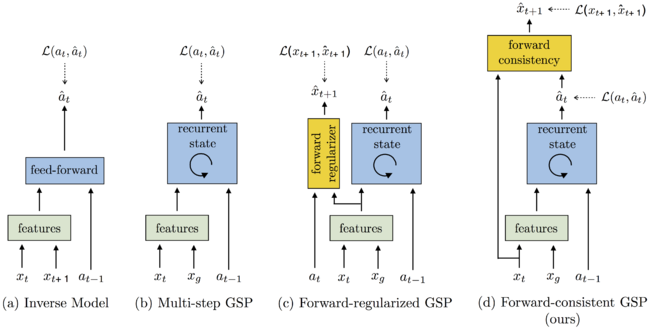
Of course, when introducing something like this forward-consistent loss, issues related to the number of steps needed to reach a certain goal become prevalent. To address this, the paper pairs the GSP with a goal recognizer that determines if the goal has been satisfied with respect to some metrics. Figure 1 shows various GSPs along with diagram d) showing the forward-consistent loss proposed in this paper.
The zero-shot imitator is tested on a Baxter robot performing tasks involving rope manipulation, a TurtleBot performing office navigation and navigation experiments in VizDoom. Positive results are shown for all three experiments leading to the conclusion that the forward-consistent GSP can be used to imitate a variety of tasks without making environmental or task-specific assumptions.
Related Work
Some key ideas related to this work are imitation learning, visual demonstration, forward/inverse dynamics and consistency and finally goal conditioning. The paper has more on each of these topics including citations to related papers. This paper is very closely related to imitation learning but the problem being addressed is different in that there is less supervision and the model requires generalization across tasks during inference.
Learning to Imitate Without Expert Supervision
In this section (and the included subsections) the methods for learning the GSP, forward consistency loss and goal recognizer network are described.
Let [math]\displaystyle{ S : \{x_1, a_1, x_2, a_2, ..., x_T\} }[/math] be the sequence of observation-action pairs generated by the agent as it explores the environment using the policy [math]\displaystyle{ a = π_E(s) }[/math]. This exploration data is used to learn the GSP.
The above equation represents the learned GSP. [math]\displaystyle{ π }[/math] takes as input a pair of observations [math]\displaystyle{ (x_i, x_g) }[/math] and outputs the sequence of required actions [math]\displaystyle{ (\overrightarrow{a}_τ : a_1, a_2, ..., a_K) }[/math] to reach the goal observation [math]\displaystyle{ x_g }[/math] from the current observation [math]\displaystyle{ x_i }[/math]. The states [math]\displaystyle{ x_i }[/math] and [math]\displaystyle{ x_g }[/math] are sampled from [math]\displaystyle{ S }[/math] and the number of actions [math]\displaystyle{ K }[/math] is inferred by the model. [math]\displaystyle{ π }[/math] can be thought of as a general deep network with parameters [math]\displaystyle{ θ_π }[/math]. It is good to note that [math]\displaystyle{ x_g }[/math] could be an intermediate subtask of the overall goal. So in essence, subtasks can be strung together to achieve an overall goal (i.e. go to position 1, then go to position 2, then go to final destination).
Let the sequence of images [math]\displaystyle{ D: \{x_1^d, x_2^d, ..., x_N^d\} }[/math] be the task to be imitated which is captured when the expert demonstrates the task. The sequence has at least one entry and can be as temporally dense as needed (i.e. the expert can show as many goals or sub-goals as needed to the agent). The agent then uses the learned GSP [math]\displaystyle{ π }[/math] to start from initial state [math]\displaystyle{ x_0 }[/math] and follow the actions predicted by [math]\displaystyle{ π(x_0, x_1^d; θ_π) }[/math] to imitate the observations in [math]\displaystyle{ D }[/math].
A separate goal recognizer network is needed to ascertain if the current observation is close to the goal or not. This is because multiple actions might be required to reach close to [math]\displaystyle{ x_1^d }[/math]. Knowing this, let [math]\displaystyle{ x_0^\prime }[/math] be the observation after executing the predicted action. The goal recognizer evaluates whether [math]\displaystyle{ x_0^\prime }[/math] is sufficiently close to the goal and if not, the agent executes [math]\displaystyle{ a = π(x_0^\prime, x_1^d; θ_π) }[/math]. This process is executed repeatedly for each image in [math]\displaystyle{ D }[/math] until the final goal is reached.
Learning the Goal-Conditioned Skill Policy (GSP)
It is easy to first describe the one-step version of GSP and then extend it to a multi-step version. The one-step trajectory can be generalized as [math]\displaystyle{ (x_t; a_t; x_{t+1}) }[/math] with GSP [math]\displaystyle{ \hat{a}_t = π(x_t; x_{t+1}; θ_π) }[/math] and is trained by the standard cross-entropy loss given below with respect to the GSP parameters [math]\displaystyle{ θ_π }[/math]:
[math]\displaystyle{ p }[/math] and [math]\displaystyle{ \hat{a}_t }[/math] are the ground-truth and predicted action distributions respectively. [math]\displaystyle{ p }[/math] is not readily available so it is empirically approximated using samples from the distribution [math]\displaystyle{ a_t }[/math]. In a standard deep learning problem it is common to assume [math]\displaystyle{ p }[/math] as a delta function at [math]\displaystyle{ a_t }[/math] but this is violated if [math]\displaystyle{ p }[/math] is multi-modal and high-dimensional. That is, the same inputs would be presented with different targets leading to high variance in gradients. This would make learning challenging, leading to the further developments presented in sections 2.2, 2.3 and 2.4.
Forward Consistency Loss
To deal with multi-modality, this paper proposes the forward consistency loss where instead of penalizing actions predicted by the GSP to match the ground truth, the parameters of the GSP are learned such that they minimize the distance between observation [math]\displaystyle{ \hat{x}_{t+1} }[/math] (prediction from executing [math]\displaystyle{ \hat{a}_t = π(x_t, x_{t+1}; θ_π) }[/math] ) and the observation [math]\displaystyle{ x_{t+1} }[/math] (ground truth). This is done so that the predicted action is not penalized if it leads to the same next state as the ground-truth action. This will in turn reduce the variation in gradients and aid the learning process. This is what is denoted as forward consistency loss.
To operationalize the forward consistency loss... The forward dynamics [math]\displaystyle{ f }[/math] are learned from the data and is defined as [math]\displaystyle{ \widetilde{x}_{t+1} = f(x_t, a_t; θ_f) }[/math]. Since [math]\displaystyle{ f }[/math] is not analytic, there is no guarantee that [math]\displaystyle{ \widetilde{x}_{t+1} = \hat{x}_{t+1} }[/math] so an additional term is added to the loss: [math]\displaystyle{ ||x_{t+1} - \hat{x}_{t+1}||_2^2 }[/math]. The parameters of [math]\displaystyle{ θ_f }[/math] are inferred by minimizing [math]\displaystyle{ ||x_{t+1} - \widetilde{x}_{t+1}||_2^2 + λ||x_{t+1} - \hat{x}_{t+1}||_2^2 }[/math] where λ is a scalar hyper-parameter. The first term ensures that the learned model explains the ground truth transitions while the second term ensures consistency. In summary, the loss function is given below:
Past works have show that learning forward dynamics in the feature space as opposed to raw observation space is more robust so this paper follows in extending the GSP to make predictions on feature representations denoted [math]\displaystyle{ \phi(x_t), \phi(x_{t+1}) }[/math]. The forward consistency loss is then computed to make predictions in the feature space \phi.
The generalization to multi-step GSP [math]\displaystyle{ π_m }[/math] is shown below where [math]\displaystyle{ \phi }[/math] refers to the feature space rather than observation space which was used in the single-step case:
The forward consistency loss is computed at each time step, t, and jointly optimized with the action prediction loss over the whole trajectory. [math]\displaystyle{ \phi(.) }[/math] is represented by a CNN with parameters [math]\displaystyle{ θ_{\phi} }[/math]. The multi-step forward consistent GSP [math]\displaystyle{ \pi_m }[/math] is implemented via a recurrent network with inputs current state, goal states, actions at previous time step and the internal hidden representation denoted [math]\displaystyle{ h_{t-1} }[/math], and outputs the actions to take.
Goal Recognizer
The goal recognizer network was introduced to figure out if the current goal is reached. This allows the agent to take multiple steps between goals without being penalized. In this paper, goal recognition was taken as a binary classification problem; given an observation and the goal, is the observation close to the goal or not. The goal classifier was trained using the standard cross-entropy loss.
Ablations and Baselines
To summarize, the GSP formulation is composed of (a) recurrent variable-length skill policy network, (b) explicitly encoding previous action in the recurrence, (c) goal recognizer, (d) forward consistency loss function, and (w) learning forward dynamics in the feature space instead of raw observation space.
To show the importance of each component a systematic ablation (removal) of components for each experiment is done to show the impact on visual imitation. The following methods will be evaluated in the experiments section:
- Classical methods: In visual navigation, the paper attempts to compare against the state-of-the-art ORB-SLAM2 and Open-SFM.
- Inverse model: Nair et al. (2017) leverage vanilla inverse dynamics to follow demonstration in rope manipulation setup.
- GSP-NoPrevAction-NoFwdConst is the removal of the paper's recurrent GSP without previous action history and without forward consistency loss.
- GSP-NoFwdConst refers to the recurrent GSP with previous action history, but without forward consistency objective.
- GSP-FwdRegularizer refers to the model where forward prediction is only used to regularize the features of GSP but has no role to play in the loss function of predicted actions.
- GSP refers to the complete method with all the components.
Experiments
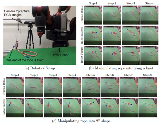
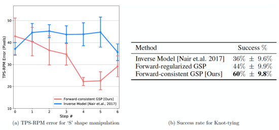
Rope Manipulation


