Understanding the Effective Receptive Field in Deep Convolutional Neural Networks
Introduction
What is the Receptive Field (RF) of a unit?
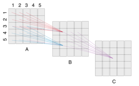
The receptive field of a unit is the region of input where the unit 'sees' and responds to. When dealing with high-dimensional inputs such as images, it is impractical to connect neurons to all neurons in the previous volume. Instead, we connect each neuron to only a local region of the input volume. The spatial extent of this connectivity is a hyper-parameter called the receptive field of the neuron (equivalently this is the filter size) [4].
Why is RF important?
The concept of receptive field is important for understanding and diagnosing how deep Convolutional neural networks (CNNs) work. Since anywhere in an input image outside the receptive field of a unit does not affect the value of that unit, it is necessary to carefully control the receptive field, to ensure that it covers the entire relevant image region. The property of receptive field allows the response is most sensitive to a local region in the image and to specific stimuli; similar stimuli trigger activations of similar magnitudes [2]. The initialization of each receptive field depends on the neuron's degrees of freedom [2]. One example outlined in this paper is that "the weights can be either of the same sign or centered with zero mean. This latter case favors a response to the contrast between the central and peripheral region of the receptive field." [2]. In many tasks, especially dense prediction tasks like semantic image segmentation, stereo and optical flow estimation, where we make a prediction for every single pixel in the input image, it is critical for each output pixel to have a big receptive field, such that no important information is left out when making the prediction.
How to increase RF size?
Make the network deeper by stacking more layers, which increases the receptive field size linearly by theory, as each extra layer increases the receptive field size by the kernel size.
Add sub-sampling layers to increase the receptive field size multiplicatively.
Modern deep CNN architectures like the VGG networks and Residual Networks use a combination of these techniques.
Intuition behind Effective Receptive Fields
The pixels at the center of a RF have a much larger impact on an output:
- In the forward pass, central pixels can propagate information to the output through many different paths, while the pixels in the outer area of the receptive field have very few paths to propagate its impact.
- In the backward pass, gradients from an output unit are propagated across all the paths, and therefore the central pixels have a much larger magnitude for the gradient from that output [More paths always mean larger gradient?].
- Not all pixels in a receptive field contribute equally to an output unit's response.
Authors prove that in many cases the distribution of impact in a receptive field distributes as a Gaussian. Since Gaussian distributions generally decay quickly from the center, the effective receptive field, only occupies a fraction of the theoretical receptive field.
The authors have correlated the theory of effective receptive field with some empirical observations. One such observation is that the random initializations lead some deep CNNs to start with a small effective receptive field, which then grows on training, which indicates a bad initialization bias.
Theoretical Results
Authors wanted to mathematically characterize how much each input pixel in a receptive field can impact the output of a unit $n$ layers up the network. More specifically, assume that pixels on each layer are indexed by $(i,j)$ with their centre at $(0,0)$. If we denote the pixel on the $p$th layer as $x_{i,j}^p$ , with $x_{i,j}^0$ as the input to the network, and $y_{i,j}=x_{i,j}^n$ as the output on the $n$th layer, we want to know how much each $x_{i,j}^0$ contributes to $y_{0,0}$. The effective receptive field (ERF) of this central output unit is then can be defined as the region containing input pixels with a non-negligible impact on it.
They used the partial derivative $\frac{\partial y_{0,0}}{\partial x_{i,j}^0}$ as the measure of such impact, which can be computed using backpropagation. Assuming $l$ as an arbitrary loss by the chain rule we can write $\frac{\partial l}{\partial x_{i,j}^0} = \sum_{i',j'}\frac{\partial l}{\partial y_{i',j'}}\frac{\partial y_{i',j'}}{\partial x_{i,j}^0}$. Now if $\frac{\partial l}{\partial y_{0,0}} =1$ and $\frac{\partial l}{\partial y_{i,j}}$ for all $i \neq 0$ and $j \neq 0$, then $\frac{\partial l}{\partial x_{i,j}^0} =\frac{\partial y_{0,0}}{\partial x_{i,j}^0}$.
For networks without nonlinearity (i.e., linear networks) this measure is independent of the input and depends only on the weights of the network.
Simplest case: Stack of convolutional layers of weights equal to 1
The authors first considered the case of $n$ convolutional layers using $k \times k$ kernels of stride 1 and a single channel on each layer and no nonlinearity, and bias.
For this special sub-case, the kernel was a $k \times k$ matrix of 1's. Since this kernel is separable to $k \times 1$ and $1 \times k$ matrices, the $2D$ convolution could be replaced by two $1D$ convolutions. This allowed the authors to focus their analysis on the $1D$ convolutions.
For this case, if we denote the gradient signal $\frac{\partial l}{\partial y_{i,j}}$ by $u(t)$ and the kernel by $v(t)$, we have
\begin{equation*} u(t)=\delta(t),\\ \quad v(t) = \sum_{m=0}^{k-1} \delta(t-m), \quad \text{where} \begin{cases} \delta(t)= 1\ \text{if}\ t=0, \\ \delta(t)= 0\ \text{if}\ t\neq 0, \end{cases} \end{equation*} and $t =0,1,-1,2,-2,...$ indexes the pixels.
The gradient signal $o(t)$ on the input pixels can now be computed by convolving $u(t)$ with $n$ $v(t)$'s so that $o(t) = u *v* ...*v$.
Since convolution in time domain is equivalent to multiplication in Fourier domain, we can write
\begin{equation*} U(w) = \sum_{t=-\infty}^{\infty} u(t) e^{-jwt}=1,\\ V(w) = \sum_{t=-\infty}^{\infty} v(t) e^{-jwt}=\sum_{m=0}^{k-1} e^{-jwm},\\ O(w) = F(o(t))=F(u(t)*v(t)*...*v(t)) = U(w).V(w)^n = \Big ( \sum_{m=0}^{k-1} e^{-jwm} \Big )^n, \end{equation*}
where $O(w)$, $U(w)$, and $V(w)$ are discrete Fourier transformations of $o(t)$, $u(t)$, and $v(t)$.
Now let us consider two non-trivial cases.
Case K=2: In this case $( \sum_{m=0}^{k-1} e^{-jwm} )^n = (1 + e^{-jw})^n$. Because $O(w)= \sum_{t=-\infty}^{\infty} o(t) e^{-jwt}= (1 + e^{-jw})^n$, we can think of $o(t)$ as coefficients of $e^{-jwt})$. Therefore, $o(t)= \begin{pmatrix} n\\t\end{pmatrix}$ is the standard binomial coefficients. As $n$ becomes large binomial coefficients distribute with respect to $t$ like a Gaussian distribution. More specifically, when $n \to \infty$ we can write
\begin{equation*}
\begin{pmatrix} n\\t \end{pmatrix} \sim \frac{2^n}{\sqrt{\frac{n\pi}{2}}}e^{-d^{2}/2n},
\end{equation*}
where $d = n-2t$ (see Binomial coefficient).
Case K>2: In this case the coefficients are known as "extended binomial coefficients" or "polynomial coefficients", and they too distribute like Gaussian [].
Random Weights
Denote $g(i, j, p) = \frac{\partial l}{\partial x_{i,j}^p}$ as the gradient on the $p$th layer, and $g(i, j, p) = \frac{\partial l}{\partial y_{i,j}}$ . Then $g(, , 0)$ is the desired gradient image of the input. The backpropagation convolves $g(, , p)$ with the $k x k$ kernel to get $g(, , p-1)$ for each p. So we can write
\begin{equation*} g(i,j,p-1) = \sum_{a=0}^{k-1} \sum_{b=0}^{k-1} w_{a,b}^p g(i+a,i+b,p), \end{equation*}
where $w_{a,b}^p$ is the convolution weight at $(a, b)$ in the convolution kernel on layer p. In this case, the initial weights are independently drawn from a fixed distribution with zero mean and variance $C$. By assuming that the gradients g are independent from the weights (linear networks only) and given that $\mathbb{E}_w[w_{a,b}^p] =0$
\begin{equation*} \mathbb{E}_{w,input}[g(i,j,p-1)] = \sum_{a=0}^{k-1} \sum_{b=0}^{k-1} \mathbb{E}_w[w_{a,b}^p] \mathbb{E}_{input}[g(i+a,i+b,p)]=0,\\ Var[g(i,j,p-1)] = \sum_{a=0}^{k-1} \sum_{b=0}^{k-1} Var[w_{a,b}^p] Var[g(i+a,i+b,p)]= C\sum_{a=0}^{k-1} \sum_{b=0}^{k-1} Var[g(i+a,i+b,p)]. \end{equation*}
Therefore, to get $Var[g(, , p-1)]$ we can convolve the gradient variance image $Var[g(, , p)]$ with a $k \times k$ kernel of 1’s, and then multiply it by $C$. Comparing this to the simplest case of all weights equal to one, we can see that the $g(, , 0)$ has a Gaussian shape, with only a slight change of having an extra $C^n$ constant factor multiplier on the variance gradient images, which does not affect the relative distribution within a receptive field.
Non-uniform Kernels
In the case of non-uniform weighting, when w(m)'s are normalized: \begin{equation*} E[S_n] = n\sum_{m=0}^{k-1} mw(m),\\ Var[S_n] = n \left (\sum_{m=0}^{k-1} m^2w(m) - \left (\sum_{m=0}^{k-1} mw(m) \right )^2 \right ), \end{equation*}
where $S_n = \sum_{i=1}^n$ $X_i$ and $X_i$’s are i.i.d. multinomial variables distributed according to $w(m)$’s, i.e. $p(X_i = m) = w(m)$.
If we take one standard deviation as the effective receptive field (ERF) size which is roughly the radius of the ERF, then this size is $\sqrt{Var[S_n]} = \sqrt{nVar[X_i]} = O(\sqrt{n})$.
Non-linear Activation Functions
The math in this section is a bit "hand-wavy", as one of their reviewers wrote, and their conclusion (Gaussian-shape ERF) is not really well backed up by their experiments. The most important point to take way form this part is that by introduction of a nonlinear activation function, the gradients depends on the network's input as well.
Verifying Theoretical Results
In all of the following experiments, a gradient signal of 1 was placed at the center of the output plane and 0 everywhere else, and then this gradient was backpropagated through the network to get input gradients. Also random inputs as well as proper random initialization of the kernels were employed.
ERFs are Gaussian distributed: By looking at the figure,
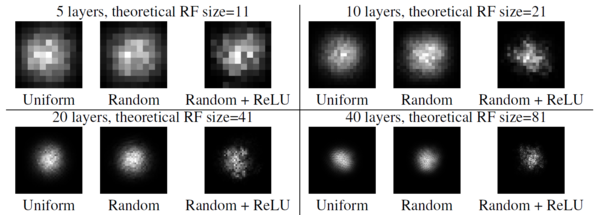
we can observe Gaussian shapes for uniformly and randomly weighted convolution kernels without nonlinear activations, and near Gaussian shapes for randomly weighted kernels with nonlinearity. Adding the ReLU nonlinearity makes the distribution a bit less Gaussian, as the ERF distribution depends on the input as well. Another reason is that ReLU units output exactly zero for half of its inputs and it is very easy to get a zero output for the center pixel on the output plane, which means no path from the receptive field can reach the output, hence the gradient is all zero. Here the ERFs are averaged over 20 runs with different random seed.
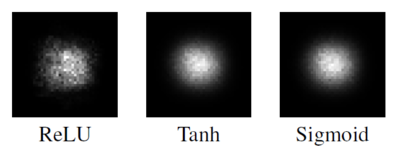
Figures below show the ERF for networks with 20 layers of random weights, with different nonlinearities. Here the results are averaged both across 100 runs with different random weights as well as different random inputs. In this setting the receptive fields are a lot more Gaussian-like.
[math]\displaystyle{ \sqrt{n} }[/math] absolute growth and [math]\displaystyle{ 1/\sqrt{n} }[/math] relative shrinkage: The figure
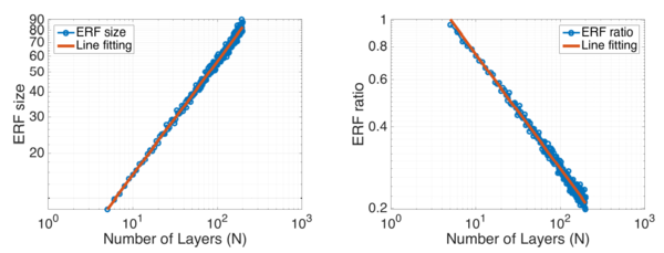
shows the change of ERF size and the relative ratio of ERF over theoretical RF wrt number of convolution layers. The fitted line for ERF size has the slope of 0.56 in log domain, while the line for ERF ratio has the slope of -0.43. This indicates ERF size is growing linearly wrt [math]\displaystyle{ \sqrt{n} }[/math] and ERF ratio is shrinking linearly wrt [math]\displaystyle{ 1/\sqrt{n} }[/math].
They used 2 standard deviations as the measurement for ERF size, i.e. any pixel with value greater than 1 - 95.45% of center point is considered in ERF. The ERF size is represented by the square root of number of pixels within ERF, while the theoretical RF size is the side length of the square in which all pixel has a non-zero impact on the output pixel, no matter how small. All experiments here are averaged over 20 runs.
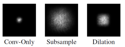
Subsampling & dilated convolution increases receptive field: The figure shows that the effect of subsampling and dilated convolution. The reference baseline is a CNN with 15 dense convolution layers. Its ERF is shown in the left-most figure. Replacing 3 of the 15 convolutional layers with stride-2 convolution results in the ERF for the ‘Subsample’ figure. Finally, replacing those 3 convolutional layers with dilated convolution with factor 2,4 and 8 gives the ‘Dilation’ figure. Both of them are able to increase the effect receptive field significantly. Note the ‘Dilation’ figure shows a rectangular ERF shape typical for dilated convolutions (why?).
How the ERF evolves during training
The authors looked at how the ERF of units in the top-most convolutional layers of a classification CNN and a semantic segmentation CNN evolve during training. For both tasks, they adopted the ResNet architecture which makes extensive use of skip-connections. As expected their analysis showed the ERF of these networks are significantly smaller than the theoretical receptive field. Also, as the networks learns, the ERF got bigger so that at the end of training was significantly larger than the initial ERF.
The classification network was a ResNet with 17 residual blocks trained on the CIFAR-10 dataset. Figure shows the ERF on the 32x32 image space at the beginning of training (with randomly initialized weights) and at the end of training when it reaches best validation accuracy. Note that the theoretical receptive field of the network is actually 74x74, bigger than the image size, but the ERF is not filling the image completely. Comparing the results before and after training demonstrates that ERF has grown significantly.

The semantic segmentation network was trained on the CamVid dataset for urban scene segmentation. The 'front-end' of the model was a purely convolutional network that predicted the output at a slightly lower resolution. And then, a ResNet with 16 residual blocks interleaved with 4 subsampling operations each with a factor of 2 was implemented. Due to subsampling operations the output was 1/16 of the input size. For this model, the theoretical RF of the top convolutional layer units was 505x505. However, as Figure shows the ERF only got a fraction of that with a diameter of 100 at the beginning of training, and at the end of training reached almost a diameter around 150.
Discussion
The Effective Receptive Field (ERF) usually decays quickly from the centre (like 2D Gaussian) and only takes a small portion of the theoretical Receptive Field (RF). This "Gaussian damage" is undesirable for tasks that require a large RF and to reduce it, the authors suggested two solutions:
- New Initialization scheme to make the weights at the center of the convolution kernel to be smaller and the weights on the outside larger, which diffuses the concentration on the center out to the periphery. One way to implement this is to initialize the network with any initialization method, and then scale the weights according to a distribution that has a lower scale at the center and higher scale on the outside. They tested this solution for the CIFAR-10 classification task, with several random seeds. In a few cases they get a 30% speed-up of training compared to the more standard initializations. But overall the benefit of this method is not always significant.
- Architectural changes of CNNs is the 'better' approach that may change the ERF in more fundamental ways. For example, instead of connecting each unit in a CNN to a local rectangular convolution window, we can sparsely connect each unit to a larger area in the lower layer using the same number of connections. Dilated convolution belongs to this category, but we may push even further and use sparse connections that are not grid-like.
Summary & Conclusion
The authors showed, theoretically and experimentally, that the distribution of impact within the receptive field (the effective receptive field) is asymptotically Gaussian, and the ERF only takes up a fraction of the full theoretical receptive field. They also studied the effects of some standard CNN approaches on the effective receptive field. They found that dropout does not change the Gaussian ERF shape. Subsampling and dilated convolutions are effective ways to increase receptive field size quickly but skip-connections make ERFs smaller.
They argued that since larger ERFs are required for higher performance, new methods to achieve larger ERF will not only help the network to train faster but may also improve performance.
Critique
The authors' finding on $\sqrt{n}$ absolute growth of Effective Receptive Field (ERF) suffers from discrepancy in ERF definition between their theoretical analysis and their experiments. Namely, in the theoretical analysis for non-uniform-kernel case they considered one standard deviation as the ERF size. However, they used two standard deviations as the measure for ERF size in the experiments.
It would be more practical if the paper also investigated the ERF for natural images (as opposed to random) as network input at least in the two cases where they examined trained networks.
The authors claim that the ERF results in the experimental section have Gaussian shapes but they never prove this claim. For example, they could fit different 2D-functions, including 2D-Gaussian, to the kernels and show that 2D-Gaussian gives the best fit. Furthermore, the pictures are given as proof of the claim that the ERF has a Gaussian distribution only show the ERF of the center pixel of the output [math]\displaystyle{ y_{0,0} }[/math]. Intuitively, the ERF of a node near the boundary of the output layer may have a significantly different shape. This was not addressed in the paper.
Another weakness is in the discussion section, where they make a connection to the biological networks. They jumped to disprove a well-observed phenomenon in the brain. The fact that the neurons in the higher areas of the visual hierarchy gradually lose their retinotopic property has been shown in a countless number of neuroscience studies. For example, grandmother cells do not care about the position of grandmother's face in the visual field. In general, the similarity between deep CNNs and biological visual systems is not as strong, hence we should take any generalization from CNNs to biological networks with a grain of salt.
Spectrograms are visual representations of audio where the axes represent time, frequency and amplitude of the frequency. The ERF of a CNN when applied to a spectrogram doesn't necessarily have to be from a Gaussian towards the center. In fact many receptive fields are trained to look for the peaks of troughs and cliffs, which essentially imply that the ERF will have more weightage towards the outside rather than the center.
References
[1] Wenjie Luo, Yujia Li, Raquel Urtasun, and Richard Zemel. "Understanding the effective receptive field in deep convolutional neural networks." In Advances in Neural Information Processing Systems, pp. 4898-4906. 2016.
[2] Buessler, J.-L., Smagghe, P., & Urban, J.-P. (2014). Image receptive fields for artificial neural networks. Neurocomputing, 144(Supplement C), 258–270. https://doi.org/10.1016/j.neucom.2014.04.045
[3] Dilated Convolutions in Neural Network - [1]
[4] http://cs231n.github.io/convolutional-networks/
[5] Thorsten Neuschel. "A note on extended binomial coefficients." Journal of Integer Sequences, 17(2):3, 2014.