This Looks Like That: Deep Learning for Interpretable Image Recognition
Presented by
Nouha Chatti
Introduction
The motivation behind this paper is to introduce a new deep learning network architecture capable of reasoning in an interpretable manner during classification tasks. The goal of the algorithm is to utilize human-understandable reasoning to perform image classification tasks.
The idea is to perform these tasks by defining a form of interpretability when processing the images. The method suggested in this paper consists of dissecting parts of the input images and comparing them to prototypical parts of training images of a given class, thus the expression "this looks like that". Interpretability is crucial in many problems that require understanding how a model makes a particular prediction. Neural networks are typically seen as some of the least interpretable models in machine learning [4]. Medical imaging is one instance where interpretability is critical, where diagnosis using X-ray scans is based on comparing to other prototypical scans. [1]
Previous Work
Interpretability in deep networks has been a long-sought goal and is a growing field of research. There already exists post-hoc interpretability methods that analyze the performance of a trained CNN, such as [2], but this type of analysis does not explain the reasoning process of how a network actually makes its decisions during classification but are rather created after this phase. There are also attention-based models that determine parts of the input they are looking at but without associating them to prototypical samples [3].
Network Architecture
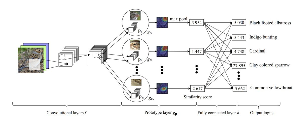
The figure below represents ProtoPNet architecture. The first layers of this network consists of commonly used convolutional layers [math]\displaystyle{ f }[/math], whose parameters are denoted [math]\displaystyle{ w_{conv} }[/math]. The layers used in this study are from the following known models VGG-16, VGG-19, ResNet-34, ResNet-152, DenseNet-121, and DenseNet-161 previously pre-trained on ImageNet which are followed by two additional 1 × 1 convolutional layers. A layer called prototype [math]\displaystyle{ g_p }[/math] is a fully connected layer h with weight [math]\displaystyle{ w_h }[/math] and no bias that returns the output prediction using a softmax function, unlike all the rest of the layers that use ReLU as the activation function. This network takes in an image [math]\displaystyle{ x }[/math] which is propagated through the convolutional layers ([math]\displaystyle{ f }[/math] of shape [math]\displaystyle{ H x W x D }[/math]) where features are extracted and learns the prototypes P of shape ([math]\displaystyle{ 1 x 1 x D }[/math]). The number of prototypes [math]\displaystyle{ m_k }[/math] is pre-defined for each class [math]\displaystyle{ k }[/math] (10 per class in this study). Each prototype will be used to represent a pattern in a patch of the conv output, corresponding to some prototypical image patch in the original pixel space. So given an output [math]\displaystyle{ z = f(x) }[/math], the j-th prototype unit [math]\displaystyle{ g_{p_{j}} }[/math] in the prototype layer [math]\displaystyle{ g_p }[/math] computes the squared L2 distances between the j-th prototype [math]\displaystyle{ p_j }[/math] and all patches of [math]\displaystyle{ z }[/math] that have the same shape as [math]\displaystyle{ p_j }[/math] and returns the similarity scores. These score values indicate the presence of the prototypical part in the image, while preserving the spatial relation of [math]\displaystyle{ z }[/math]. It is possible to up-sample it to the original size in order to obtain a heatmap with different parts that are most similar to the compared prototypes. The scores given by each unit are produced using max-pooling to obtain a single score of how strong a prototypical pattern is present in the specific patch of the input, which are then multiplied by the weight matrix [math]\displaystyle{ w_h }[/math] in [math]\displaystyle{ h }[/math] to produce the output logits as shown in Figure 1.

Training Algorithm
The network is trained in three stages. First, stochastic gradient descent (SGD) of all but the last layers, followed by projection of the prototypes, and lastly convex optimization. In the initial stage the model identifies the most significant patches for the classification task and distinguishes between the prototypes of the images' true classes and those that are from different classes. SGD is used to optimize the parameters from the convolution layers and the prototypes of the prototype layer while fixing the weights of the fully connected layer in order to make the network learn to decrease the predicted probability when a part of an image of a given class is similar to a prototype from a different class. As for the second stage the aim is to visualize and associate each prototype with the most similar training image patch using the following update for every prototype of a class k: [math]\displaystyle{ P_j = \underset{z\ in Z_j}{\operatorname{arg\,min}} \lVert{z -p_j}\rVert_2 \quad\textrm{where}\quad Z_j = \{z:z \in \quad\textrm{patches} (f(x_i)) \forall i \quad\textrm{s.t}\quad y_i=k \} }[/math] During this stage, associating a patch of the training image x to its corresponding prototype p is done as a result of the activation. The patch of x that is selected is the one that p activates the most given the activation map of x by p. In the last training stage, convex optimization is applied on the last layer while fixing parameters of previous layers, to improve accuracy by adding sparsity to the model. In other words, it prevents the model from classifying an image to a particular class because it does not have prototypes from other classes. The optimization problem that they try to solve is:

Datasets
The datasets that were used in this study are CUB-200-2011 representing images of 200 bird species as well as the Stanford Cars dataset with 196 car models. Data augmentation techniques were applied to enlarge both training datasets. The following are two examples of the classification task process of images from both datasets and the process of decision making.
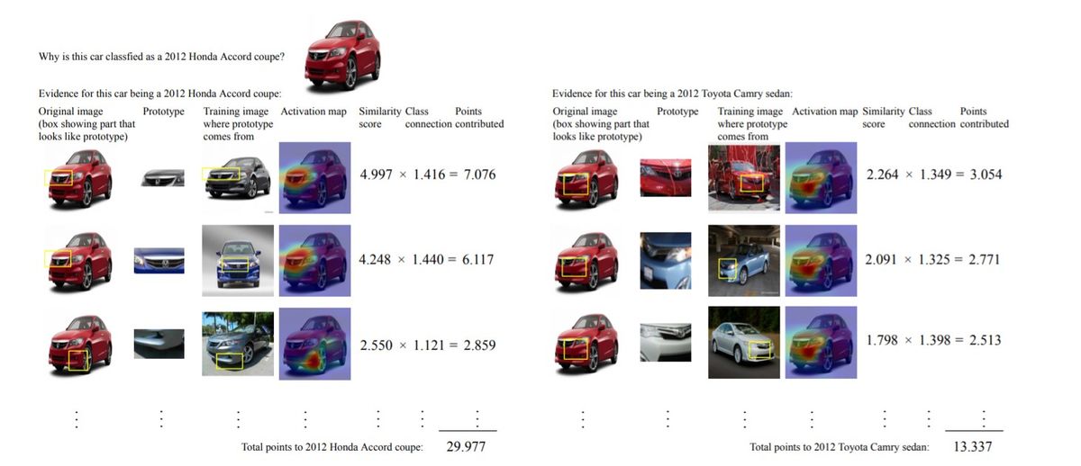
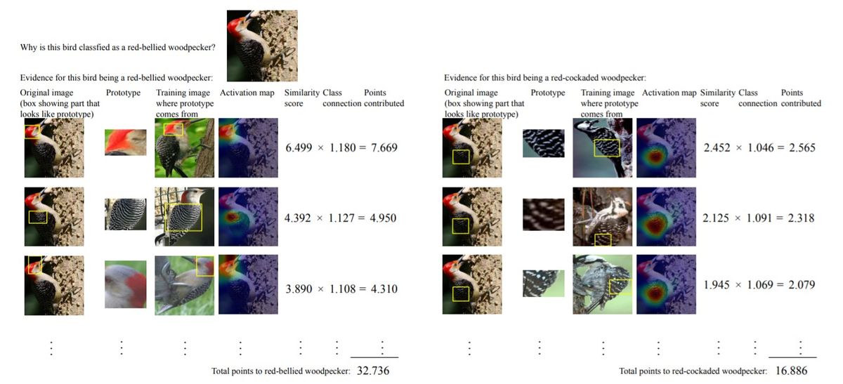
Examples of reasoning process: As it is shown in the figure below, given the testing image, the model first compares it to all learned prototypes (from all classes), looking to find proof to the image belonging to a certain class k by using the prototypes of class k. The comparison returns the similarity scores with each prototype pi and looks for the part of the image that is the most activated by pi. These scores are weighted and summed to correctly classify the testing image.


Results
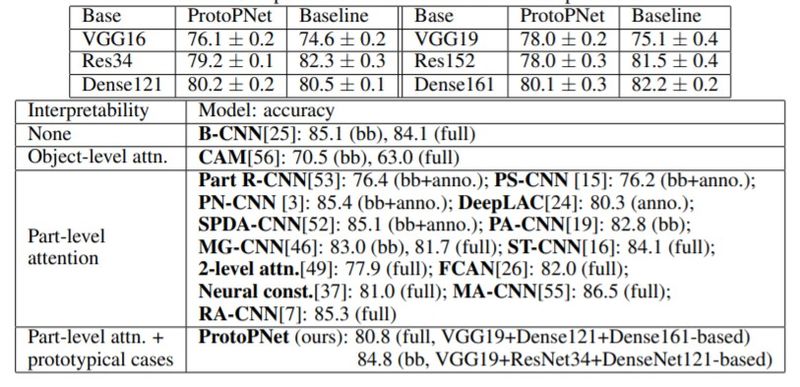
The results obtained using ProtoPNet on bird images as well as the car models are compared to the baseline models as well as attention-based deep models that were trained on the same datasets that ProtoPNet was trained on. ProtoPNet accuracy results are very close and as good as the non-interpretable baselines as shown in the tables below.


Another experience of combining many protoPNet models shows an improvement of the accuracy while preserving the transparency of the decision making process. The paper implemented the model with similar architecture as ALL-CNN-V network and obtains a prediction rate 89.30% in cifar-10 dataset.
Conclusion
The aim of constructing the ProtoPNet network was to introduce the interpretability property to neural networks. It is able to dissect images to find prototypical parts. The predictions of an image are made based on a comparison of parts of this image and learned prototypes of each class. One of the greatest advantages of ProtoPNet is that it allows the user to observe the process of how the model is making predictions and therefore understands the reasoning in case of misclassification errors. However, one disadvantage of this network is the addition of another hyperparameter in the form of the number of prototypes.
Critique
I think that this is a really interesting approach to provide insights as to why a neural network made a certain prediction. Intuitively, based on the architecture, it seems that each convolutional layer learns a certain "aspect" of the image (ie. wheel of a car, the beak of the bird, etc). It would be interesting to see how much further one can take this idea, especially in classifying images of things that appear very similar to the human eye (i.e. various insects).
Source code
The code for this paper is available at https://github.com/cfchen-duke/ProtoPNet
Refrences
[1] C. Chen, O. Li, A. Barnett, J. Su, C. Rudin, This looks like that: deep learning for interpretable image recognition, arXiv preprint, arXiv:1806.10574, 2018.
[1] A. Holt, I. Bichindaritz, R. Schmidt, and P. Perner. Medical applications in case-based reasoning. The Knowledge Engineering Review, 20:289–292, 09 2005.
[2] K. Simonyan, A. Vedaldi, and A. Zisserman. Deep Inside Convolutional Networks: Visualising Image Classification Models and Saliency Maps. In Workshop at the 2nd International Conference on Learning Representations (ICLR Workshop), 2014
[3] B. Zhou, A. Khosla, A. Lapedriza, A. Oliva, and A. Torralba. Learning Deep Features for Discriminative Localization. In Proceedings of the IEEE Conference on Computer Vision and Pattern Recognition (CVPR), pages 2921–2929. IEEE, 2016
[4] Molnar, Christoph. "Interpretable machine learning. A Guide for Making Black Box Models Explainable", 2019. https://christophm.github.io/interpretable-ml-book/