The Detection of Black Ice Accidents Using CNNs: Difference between revisions
| (4 intermediate revisions by one other user not shown) | |||
| Line 1: | Line 1: | ||
== Presented by == | == Presented by == | ||
Ann Gie Wong, Hannah Kerr, Shao Zhong Li | |||
== Introduction == | == Introduction == | ||
| Line 59: | Line 61: | ||
To assist in feature extraction, objects such as road structures, lanes, and shoulders within each image were removed so that the road characteristics of interest can be clearly identified. | To assist in feature extraction, objects such as road structures, lanes, and shoulders within each image were removed so that the road characteristics of interest can be clearly identified. | ||
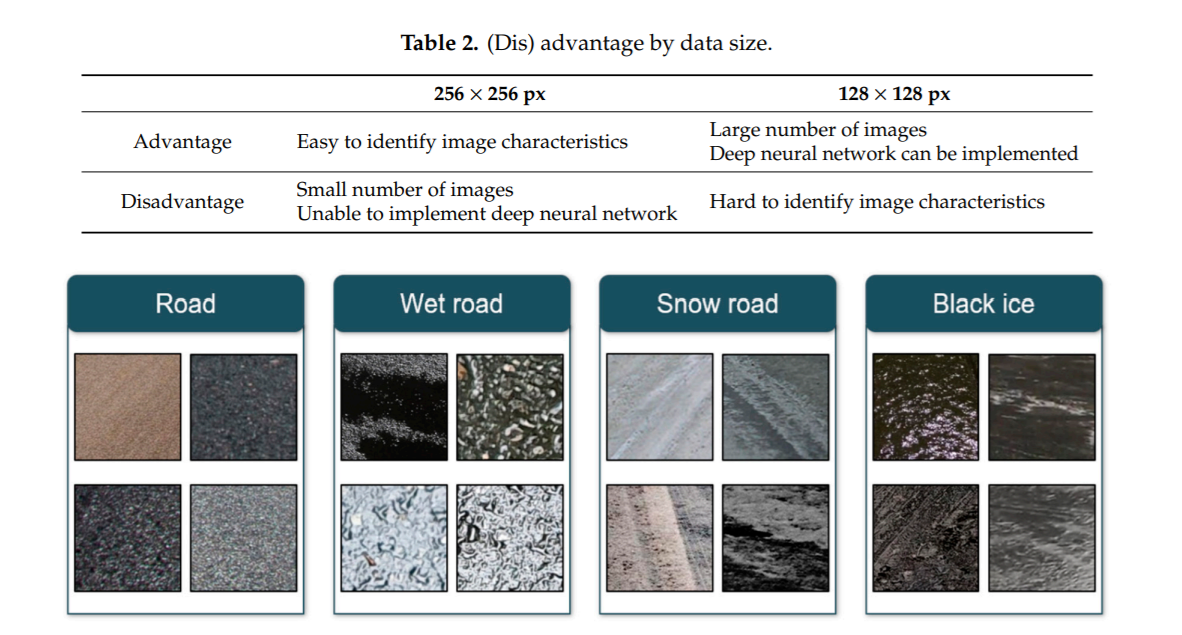
Consideration was given in the decision of the image size by weighing the pros and cons. In general, making images smaller will cause a loss of information. However, smaller image sizes allow for a larger number of images and deep neural network implementations. On the other hand, when the image size is large, feature extraction can be more accurate as the finer features are not lost, and the network can learn more robust features, but the disadvantage is that the number of images is reduced, and a deep neural network is difficult to implement. In this study, a 128 x 128 px size is selected to proceed with training. The results of the data split are shown in Figure 2. | Consideration was given in the decision of the image size by weighing the pros and cons. In general, making images smaller will cause a loss of information. However, smaller image sizes allow for a larger number of images and deep neural network implementations. On the other hand, when the image size is large, feature extraction can be more accurate as the finer features are not lost, and the network can learn more robust features, but the disadvantage is that the number of images is reduced, and a deep neural network is difficult to implement. In this study, a 128 x 128 px size is selected to proceed with training. The results of the data split are shown in Figure 2. | ||
[[File:DBIAPAVUCNN table 2.png]] | |||
<b> 1st Preprocessing </b> | <b> 1st Preprocessing </b> | ||
| Line 68: | Line 73: | ||
The color image of 128 × 128 px obtained earlier through data split has the advantage of having three channels available to help identify the characteristics. However, because of the three channels of data, the size of the data is large, which limits the number of training data and the implementation of deep neural networks. Therefore, this study has transformed the data into grayscale image data. | The color image of 128 × 128 px obtained earlier through data split has the advantage of having three channels available to help identify the characteristics. However, because of the three channels of data, the size of the data is large, which limits the number of training data and the implementation of deep neural networks. Therefore, this study has transformed the data into grayscale image data. | ||
[[File:DBIAPAVUCNN table 3.png]] | |||
2. Data padding | 2. Data padding | ||
| Line 74: | Line 81: | ||
Therefore, in this study, the image data were padded to prevent distortion of the edges of the data. | Therefore, in this study, the image data were padded to prevent distortion of the edges of the data. | ||
[[File:DBIAPAVUCNN table 4.png]] | |||
<b> 2nd preprocessing </b> | <b> 2nd preprocessing </b> | ||
After the 1st preprocessing, during which channel setup and data padding were performed, image data of 150 x 150 px in GRAYSCALE format were obtained with the following categories: 4900 road and wet road image data and | After the 1st preprocessing, during which channel setup and data padding were performed, image data of 150 x 150 px in GRAYSCALE format were obtained with the following categories: 4900 road and wet road image data and 3900 snow road and black ice image data (Table 5). | ||
[[File:DBIAPAVUCNN table 5.png]] | |||
3. Data Augmentation | 3. Data Augmentation | ||
| Line 86: | Line 97: | ||
Data augmentation would help greatly, especially for this study, which aims to identify black ice, which is not only seasonal but also reliant on very specific conditions to form, thus making image data on black ice more sparse relative to other types of data. To improve the accuracy of CNN, the ImageDataGenerator function provided by the Keras library was used to augment the data under the conditions in (Table 6). | Data augmentation would help greatly, especially for this study, which aims to identify black ice, which is not only seasonal but also reliant on very specific conditions to form, thus making image data on black ice more sparse relative to other types of data. To improve the accuracy of CNN, the ImageDataGenerator function provided by the Keras library was used to augment the data under the conditions in (Table 6). | ||
[[File:DBIAPAVUCNN table 6.png]] | |||
The process of building the training data through data augmentation is as follows. | The process of building the training data through data augmentation is as follows. | ||
From the original 17,600 sheets of data, 1000 were randomly extracted from each class and designated as test data. The rest of the data, which is the training data, was augmented using the ImageDataGenerator function, which increases the total number of images to 10,000 per class. Then, from there, the data was split into the train data and validation data at a ratio of 8:2. Therefore, the final ratio of train, validation, and test data for each class was 8:2:1. (Figure 3 and Table 7). | From the original 17,600 sheets of data, 1000 were randomly extracted from each class and designated as test data. The rest of the data, which is the training data, was augmented using the ImageDataGenerator function, which increases the total number of images to 10,000 per class. Then, from there, the data was split into the train data and validation data at a ratio of 8:2. Therefore, the final ratio of train, validation, and test data for each class was 8:2:1. (Figure 3 and Table 7). | ||
[[File:DBIAPAVUCNN table 7.png]] | |||
== Model Architecture == | == Model Architecture == | ||
| Line 100: | Line 115: | ||
Finally, the Stochastic Gradient Descent Optimizer was used, and 200 epochs were applied using a batch-size of 32. The model training is stopped if the validation loss does not fall below the minimum value encountered so far within 20 epochs. | Finally, the Stochastic Gradient Descent Optimizer was used, and 200 epochs were applied using a batch-size of 32. The model training is stopped if the validation loss does not fall below the minimum value encountered so far within 20 epochs. | ||
[[File:DBIAPAVUCNN figure 4.png]] | |||
== Results == | == Results == | ||
| Line 105: | Line 122: | ||
The loss reported with the optimal model was found to be 0.008 and 0.097 with accuracy 0.998 and 0.982. A loss/accuracy graph over time and confusion matrix is included as follows. The confusion matrix evaluates the accuracy rate between each 2 pairs of the 4 classes. This allows us to analyze patterns and mis-classification behaviour by the model between each 2 pairs. | The loss reported with the optimal model was found to be 0.008 and 0.097 with accuracy 0.998 and 0.982. A loss/accuracy graph over time and confusion matrix is included as follows. The confusion matrix evaluates the accuracy rate between each 2 pairs of the 4 classes. This allows us to analyze patterns and mis-classification behaviour by the model between each 2 pairs. | ||
Moreover, the precision and recall rates are reported for a more holistic view of the model’s performance for each class. We see that the model produces a low amount of false positives and false negatives, scoring quite high on precision and recall for each of the 3 classes. | [[File:DBIAPAVUCNN figure 5.png]] | ||
[[File:DBIAPAVUCNN table 9.png]] | |||
Moreover, the precision and recall rates are reported for a more holistic view of the model’s performance for each class. We see that the model produces a low amount of false positives and false negatives, scoring quite high on precision and recall for each of the 3 classes. | |||
[[File:DBIAPAVUCNN table 10.png]] | |||
== Conclusion == | == Conclusion == | ||
Latest revision as of 15:54, 14 November 2021
Presented by
Ann Gie Wong, Hannah Kerr, Shao Zhong Li
Introduction
As automated vehicles become more popular it is critical for these cars to be tested on every realistic driving scenario. Since AVs aim to improve safety on the road they must be able to handle all kinds of road conditions. One way an AV can prevent an accident is going from a passive safety system to an active safety system once a risk is identified.
Every country has their own challenges and in Canada for example, AVs need to understand how to drive in the winter. However, not enough testing and training has been done to mitigate winter risks. Black ice is one of the leading causes of accidents in the winter and is very challenging to see since it is a thin, transparent layer of ice. Because of this, focus needs to be placed on AVs identifying black ice.
Previous Work
In the past other methods of detecting black ice included using:
- Sensors
- Electric current sensors imbedded in concrete
- Change of electrical current resistance between stainless steel columns inside the concrete based on how what is on top of the road
- Sound Waves:
- Used 3 different soundwaves
- Road conditions detected through reflectance of the waves
- To be used for basic data in the development of road condition detectors
- Light Sources
- Different road conditions have unique light reflection
- Specular and diffuse reflections
- Types of ice were classified based on thickness and volume
- Other road conditions could be determined through reflection as well
Transportation in general has been using artificial intelligence for many different purposes.
Vehicle and pedestrian detection has been using various forms of convolutional neural networks like AlexNet, YOLO, R-CNN, Faster R-CNN, etc. Some models had better performance whereas others had a faster processing time but overall great success has been achieved.
In addition, the identification of traffic signs has had studies using similar CNN structures. These algorithms are able to process high-definition images quickly and recognize the boundary of the traffic sign allowing for quick processing.
Lastly, the detection of cracks in the road used CNN algorithms to identify the existence of a crack and classifying the it’s length with a maximum misclassification of 1cm.
Significant progress has been made for transportation but there is a lack of training on winter roads and black ice specifically. Since CNN has great success with quickly identifying objects of interest in images, using CNN for black ice detection and accident prevention is a natural extension.
Data collection
CNN is a popular class of Artificial Neural Networks (ANN) that is commonly used in image analysis due to its excellent performance in object detection using images.It differs from ANN in that it maintains and delivers spatial information on images by adding synthetic and pooling layers to a normal ANN. As mentioned earlier, various studies regarding the transportation sector had used CNN, but the study of black ice detection on the road has only thus far been conducted using other methodologies (sensors and optics). This study aims to detect black ice by utilizing CNN on images of various road conditions.. In this chapter, the details of data collection, 1st preprocessing, and 2nd preprocessing, how the model was designed, and the training undertaken (see Figure 1) are discussed.
1. Data Collection
Image data was collected using Google Image Search for four categories of road condition: road, wet road, snow road and black ice. Images were of different regions and road environments and make up a total of 2230 images.
2. Data Split
To assist in feature extraction, objects such as road structures, lanes, and shoulders within each image were removed so that the road characteristics of interest can be clearly identified.
Consideration was given in the decision of the image size by weighing the pros and cons. In general, making images smaller will cause a loss of information. However, smaller image sizes allow for a larger number of images and deep neural network implementations. On the other hand, when the image size is large, feature extraction can be more accurate as the finer features are not lost, and the network can learn more robust features, but the disadvantage is that the number of images is reduced, and a deep neural network is difficult to implement. In this study, a 128 x 128 px size is selected to proceed with training. The results of the data split are shown in Figure 2.
1st Preprocessing
In the 1st stage of Preprocessing, the channel was set up and data padding was performed on the training data.
1. Channel Setup
The color image of 128 × 128 px obtained earlier through data split has the advantage of having three channels available to help identify the characteristics. However, because of the three channels of data, the size of the data is large, which limits the number of training data and the implementation of deep neural networks. Therefore, this study has transformed the data into grayscale image data.
2. Data padding
Data padding is used to resize training images by adding spaces and meaningless symbols to the end of existing data. When training was done without data padding, very low accuracy (25%) and high loss values were achieved (Table 4). This is because the edges of the image data are distorted by the data enhancement.
Therefore, in this study, the image data were padded to prevent distortion of the edges of the data.
2nd preprocessing
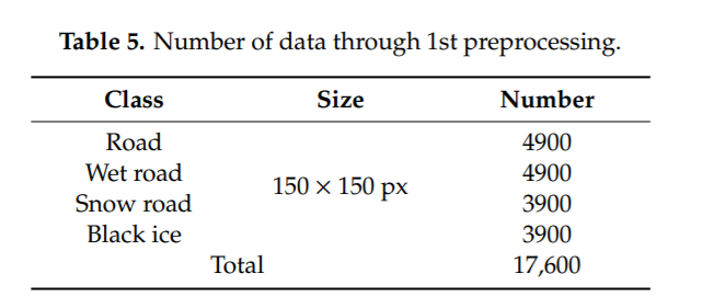
After the 1st preprocessing, during which channel setup and data padding were performed, image data of 150 x 150 px in GRAYSCALE format were obtained with the following categories: 4900 road and wet road image data and 3900 snow road and black ice image data (Table 5).
3. Data Augmentation
In the 2nd preprocessing stage, to improve the diversity in the image data obtained through Google Image Search, additional image data was created through data augmentation on existing image data.
This is done in hopes to improve the accuracy of the model since large amounts of data are essential for high accuracy and prevention of overfitting.
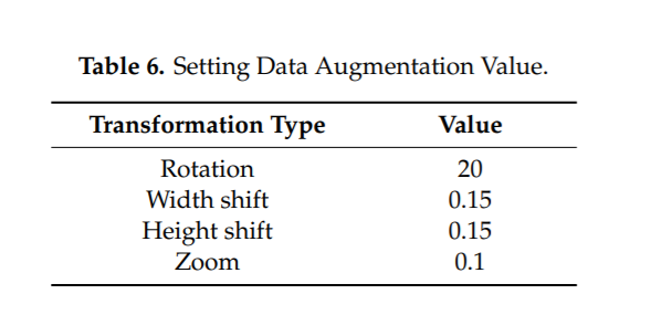
Data augmentation would help greatly, especially for this study, which aims to identify black ice, which is not only seasonal but also reliant on very specific conditions to form, thus making image data on black ice more sparse relative to other types of data. To improve the accuracy of CNN, the ImageDataGenerator function provided by the Keras library was used to augment the data under the conditions in (Table 6).
The process of building the training data through data augmentation is as follows.
From the original 17,600 sheets of data, 1000 were randomly extracted from each class and designated as test data. The rest of the data, which is the training data, was augmented using the ImageDataGenerator function, which increases the total number of images to 10,000 per class. Then, from there, the data was split into the train data and validation data at a ratio of 8:2. Therefore, the final ratio of train, validation, and test data for each class was 8:2:1. (Figure 3 and Table 7).
Model Architecture
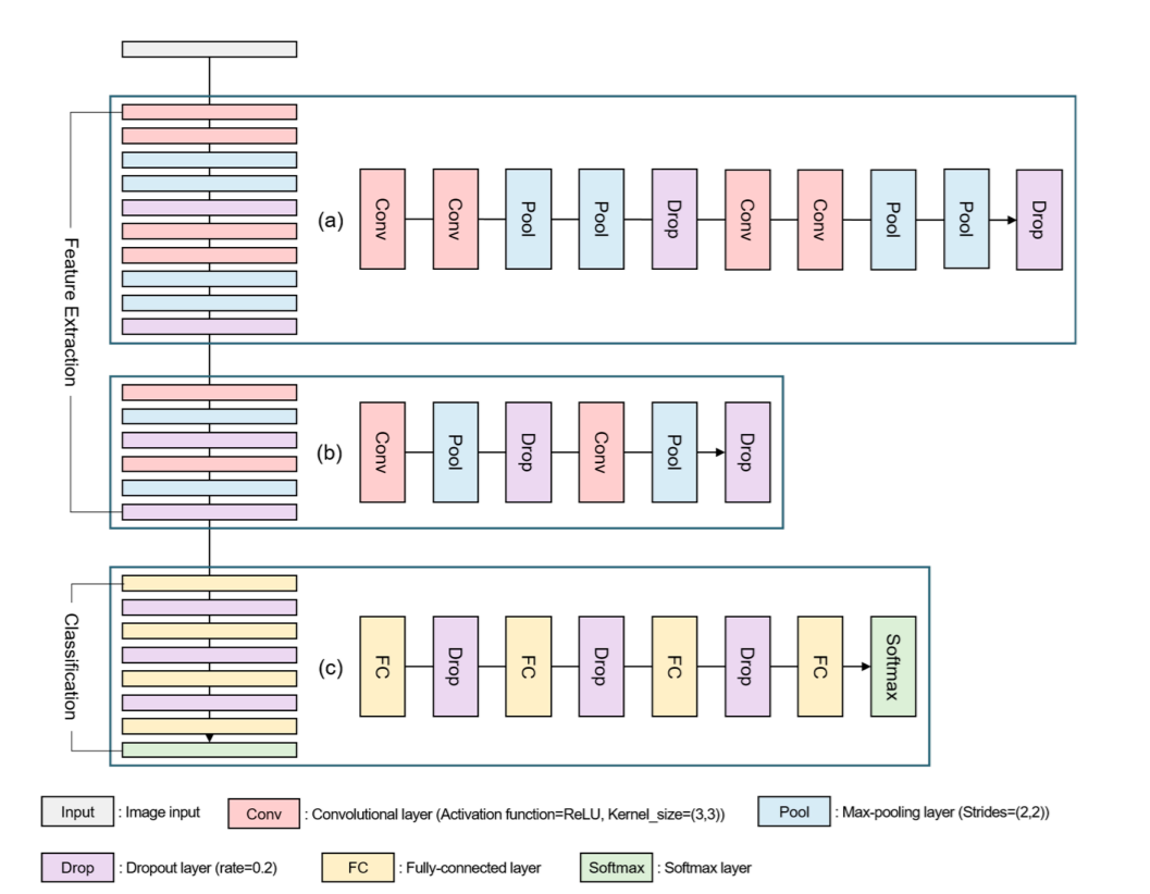
The model structure consists of 2 main components: Feature extraction and Classification. The Feature extraction component can be broken down into 2 sections. The model begins with 2 convolutional layers, using a 3x3 kernel size, paired with the ReLU activation function to avoid vanishing gradients. The goal of the convolutional layers is to extract the main features from the input image like edges, orientation, color, and other important features to distinguish black ice. It is followed by 2 max-pooling layers with a 2x2 stride. The pooling layers map the grid of values in each window to a single output value, reducing the output size of the convolutional layers. This allows the most relevant features to be picked out while reducing the amount of computation needed downstream. The max-pooling operation is used which will yield only the maximum value out of each window. A 20% dropout layer is then used, which randomly “drops” 20% of the weights from the previous convolutional layers during training which aims to improve generalization and avoid over-fitting. This structure is then repeated, making up the first component of the Feature Extraction workflow.
The previous layout is then repeated but with 1 convolutional layer, followed by one max-pooling layer, instead of 2, and one Dropout layer with the same parameters.
The classification component of the architecture consists of fully connected layers feeding into a softmax’ed output. There are 4 fully-connected layers with 3 dropout layers in between.
Finally, the Stochastic Gradient Descent Optimizer was used, and 200 epochs were applied using a batch-size of 32. The model training is stopped if the validation loss does not fall below the minimum value encountered so far within 20 epochs.
Results
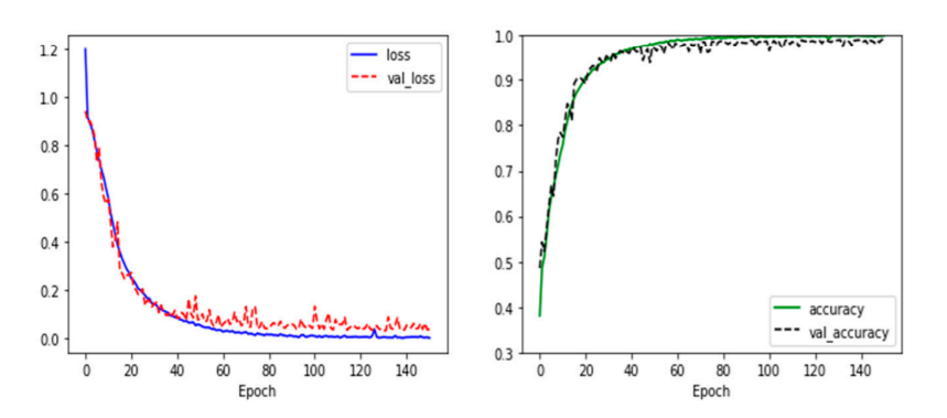
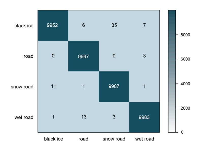
The loss reported with the optimal model was found to be 0.008 and 0.097 with accuracy 0.998 and 0.982. A loss/accuracy graph over time and confusion matrix is included as follows. The confusion matrix evaluates the accuracy rate between each 2 pairs of the 4 classes. This allows us to analyze patterns and mis-classification behaviour by the model between each 2 pairs.
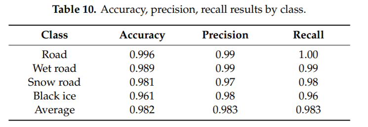
Moreover, the precision and recall rates are reported for a more holistic view of the model’s performance for each class. We see that the model produces a low amount of false positives and false negatives, scoring quite high on precision and recall for each of the 3 classes.
Conclusion
In this study, CNN was used to detect black ice which can be difficult to detect by the naked eye, with the goal to prevent black ice accidents in AVs. Data were collected and classified into four classes, and the train, validation, and test data of each class were obtained after data pre-processing was performed in the order of data split, data padding, and data augmentation.
Unlike the DCNN model, the CNN model proposed in this study was designed to be relatively simple yet robust, with an accuracy of about 96%.
This study is significant in that black ice, which is a significant risk factor even in the era of AVs, was detected using AI, not sensors and wavelengths. It is expected that this will prevent black ice accidents of AVs and will be used as basic data for future convergence research.
Overall, the CNN-based black ice detection method can be applied through deploying the CNN process on AVs and CCTVs as part of an early-warning system. Approaching vehicles can then be made aware in advance the possibility of black ice presence in the area, and the drivers will be able to take preventative measures like slowing down, more careful steering, etc.
Critiques
Due to the choice of using GRAYSCALE images of black ice, which is mainly formed at dawn, the resulting model has a tendency to get some classes mixed up due to the loss of light characteristics in the training data. The shimmers found in the snow road due to light reflection are absent when the same image is converted into grayscale, resulting in the model not able to correctly distinguish one from the other. Therefore, further research needs to be conducted to find the optimal neural network that utilizes RGB images to detect black ice.
Also, since the data were collected through Google Image Search, only images that are taken relatively close to the road are used in the training of the model. Therefore, further research needs to be conducted to construct a CNN model applicable to various situations by varying the distance and angle to the road to be detected [48–50] in the image data.
References
[1] Hojun Lee, Minhee Kang, Jaein Song, and Keeyeon Hwang. The Detection of Black Ice Accidents for Preventative Automated Vehicles Using Convolutional Neural Networks. 2020.


