STAT946F17/ Learning a Probabilistic Latent Space of Object Shapes via 3D GAN: Difference between revisions
No edit summary |
No edit summary |
||
| Line 8: | Line 8: | ||
= Methodology = | = Methodology = | ||
Let us first review Generative Adversarial Networks (GANs). As proposed in Goodfellow et al. [2014], GANs consist of a generator and a discriminator, where the discriminator tries to classify real objects and objects synthesized by the generator, while the generator attempts to confuse the discriminator. With proper guidance, this adversarial game will result in a generator the is able to synthesize fake samples very similar to the real training samples that the discriminator cannot distinguish. | Let us first review Generative Adversarial Networks (GANs). As proposed in Goodfellow et al. [2014], GANs consist of a generator and a discriminator, where the discriminator tries to classify real objects and objects synthesized by the generator, while the generator attempts to confuse the discriminator. With proper guidance, this adversarial game will result in a generator the is able to synthesize fake samples very similar to the real training samples that the discriminator cannot distinguish. This can be thought of as a zero-sum or minimax two player game. The analogy typically used is that the generative model is like ``a team of counterfeiters, trying to produce and use fake currency'' while the discriminative model is like ``the police, trying to detect the counterfeit currency''. The generator is trying to fool the discriminator while the discriminator is trying to not get fooled by the generator. As the models train through alternating optimization, both methods are improved until a point where the “counterfeits are indistinguishable from the genuine articles”. | ||
=== 3D-GANs === | === 3D-GANs === | ||
In this paper, 3D Generative Adversarial Networks (3D-GANs) are presented as a simple extension of GANs for 2D imagery. Here, the model is composed of i) a generator (G) which maps a 200-dimensional latent vector z | In this paper, 3D Generative Adversarial Networks (3D-GANs) are presented as a simple extension of GANs for 2D imagery. Here, the model is composed of i) a generator (G) which maps a $200$-dimensional latent vector z to a $64 \times 64 \times 64$ cube, representing the object $G(z)$ in voxel space, and ii) a discriminator (D) which outputs a confidence value $D(x)$ of whether a 3D object input x input is real or synthetic. Following Goodfellow et al. [2014], the classification loss used at the end of the discriminator is binary cross-entropy as | ||
$L_{3D-GAN} = \log D(x) + \log( 1 - D( G(z) ) )$ | $L_{3D-GAN} = \log D(x) + \log( 1 - D( G(z) ) )$ | ||
where $x$ is a real object in a $64 \times 64 \times 64$ space, and $z$ is randomly sampled noise from a distribution $p(z)$. In this work coefficients of $z$ are randomly sampled from a probabilistic latent space (Uniform $[0,1]$). | |||
% \[ | % \[ | ||
| Line 27: | Line 31: | ||
An extension of ... | An extension of ... | ||
= Training | |||
= Training Details = | |||
=== Network Architecture === | === Network Architecture === | ||
===== Generator ===== | ===== Generator ===== | ||
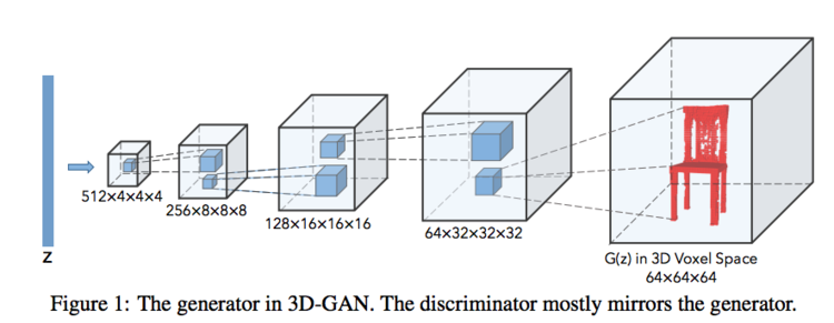
[[File:amirhk_network_arch.png| | The generator used in 3D-GAN follows the architecture of Radford et al.'s [2016] all-convolutional network, a neural network with no fully-connected and no pooling layers. As portrayed in Figure 1, this network comprises of $5$ volumetric fully convolutional layers with kernels of size $4 \times 4 \times 4$ and stride 2. Batch normalization and ReLU layers ($f(x) = \mathbb{1}(x \ge 0)(x)$) are present after every layer, and the final convolution layer is appended with a Sigmoid layer. The input is a $200$-dimensional vector and the output is $64 \times 64 \times 64$ matrix with values in $[0,1]$. | ||
[[File:amirhk_network_arch.png|right|750px]] | |||
===== Discriminator ===== | ===== Discriminator ===== | ||
===== Encoder ===== | The discriminator mostly mirrors the generator. This network takes a $64 \times 64 \times 64$ matrix as input and outputs a real number in $[0,1]$. Instead of ReLU activation function, the discriminator has leaky ReLU layers ($f(x) = \mathbb{1}(x \lt 0)(\alpha x) + \mathbb{1}(x \ge 0)(x)$) with $\alpha = 0.2$. Batch normalization layers and Sigmoid layers are consistent in both the generator and discriminator networks. | ||
===== Image Encoder ===== | |||
Finally, the image encoder in the VAE network takes as input an RGB image of size $256 \times 256 \times 3$ and outputs a $200$-dimensional vector. This network again consists of $5$ spatial (not volumetric) convolutional layers with numbers of channels $\{64, 128, 256, 512, 400\}$, kernel sizes $\{11, 5, 5, 5, 8\}$, and strides $\{4, 2, 2, 2, 1\}$, respectively. ReLU and batch normalization layers are interspersed between every convolutional layer. While the output of this image encoder is $200$-dimensional, the final layer outputs a $400$-dimensional vector that represents a $200$-dimensional Gaussian (split evenly to represent the mean and diagonal covariance). This is a common component of variational auto-encoder networks. Therefore, a final sampling layer is appended to the last convolutional layer to sample a $200$-dimensional vector from the Gaussian distribution, which is later used by the 3D-GAN. | |||
=== Coupled Generator-Discriminator Training === | === Coupled Generator-Discriminator Training === | ||
| Line 45: | Line 61: | ||
The approach used in this paper is interesting in that it adaptively decides whether to train the network or not. Here, for each batch, D is only updated if its accuracy in the last batch is <= 80%. Additionally, the generator learning rate is set to 2.5 x 10e-3 whereas the discriminator learning rate is set to 10e-5. This further caps the speed of training for the discriminator relative to the generator. | The approach used in this paper is interesting in that it adaptively decides whether to train the network or not. Here, for each batch, D is only updated if its accuracy in the last batch is <= 80%. Additionally, the generator learning rate is set to 2.5 x 10e-3 whereas the discriminator learning rate is set to 10e-5. This further caps the speed of training for the discriminator relative to the generator. | ||
=== | |||
= Evaluation = | |||
To assess the quality of 3D-GAN and 3D-VAE-GAN, the authors perform the following set of experiments | |||
# Qualitative results for 3D generated objects | |||
# Classification performance of learned representations w/o supervision | |||
# 3D object reconstruction from a single image | |||
# Analyzing learned representations for generator and discriminator | |||
Each of these experiments has a dedicated section below with experiment setup and results. First, we shall introduce the datasets used across these experiments. | |||
===== Datasets ===== | |||
* ModelNet 10 & ModelNet 40 [Wu et al., 2016] | |||
** A comprehensive and clean collection of 3D CAD models for objects used as popular benchmark | |||
** List of the most common object categories in the world | |||
** 3D CAD models belonging to each object category using online search engines by querying for each object category | |||
** Manually annotated using hired human workers on Amazon Mechanical Turk to decide whether each CAD model belongs to the specified cateogries | |||
** ModelNet 10 & ModelNet 40 datasets completely cleaned in-house | |||
** Orientations of CAD models in ModelNet 10 are also manually aligned | |||
* ShapeNet [Chang et al., 2015] | |||
** Clean 3D models and manually verified category and alignment annotations | |||
** 55 common object categories with about 51,300 unique 3D models | |||
** Collaborative effort between researchers at Princeton, Stanford and Toyota Technological Institute at Chicago (TTIC) | |||
* IKEA Dataset [supplied by author] | |||
** 1039 objects centre-cropped from 759 images | |||
** Images captured in the wild, often w/ cluttered backgrounds and occluded | |||
** 6 categories: bed, bookcase, chair, desk, sofa, table | |||
===== Qualitative results for 3D generated objects ===== | ===== Qualitative results for 3D generated objects ===== | ||
| Line 85: | Line 148: | ||
[[File:amirhk_eval_3.png|800px]] | [[File:amirhk_eval_3.png|800px]] | ||
===== Analyzing learned representations for generator and discriminator ===== | |||
In this section we explore the learned representations of the generator and discriminator in a trained 3D-GAN. Starting with a $200$-dimensional vector as input, the generator neurons will fire to generate a 3D object, consequently leading to the firing of neurons in the discriminator which will produce a confidence value between $[0,1]$. To understand the latent space of vectors for object generation, we first vary the intensity of each dimension in the latent vector and observe the effect on the generated 3D objects. In Figure 5, each red region marks the voxels affected by changing values in a particular dimesnion of the latent vector. It can be seen that semantic meaning such as width and thickness of surfaces is encoded in each of these dimensions. | |||
[[File:amirhk_representations_gen_1.png|800px]] | |||
Next, we explore intra-class and inter-class object metamorphosis by interpolating between latent vector representation of a source and target 3D object. In Figure 6, we see a smooth transition exists for various types of chairs (w/ and w/o arm rests, and with varying backrest), as well as for a smooth transition between race car and speedboat. | |||
[[File:amirhk_representations_gen_2.png|700px]] | |||
Next, as is common in generative model evaluations, a simple arithmetic scheme is tested on latent vector representation of 3D objects. In Figure 8 shows that not only are generative networks able to encode semantic knowledge of chair and face images in its latent space, but these learned representations behave similarly as well. This can be seen because simple arithmetic on latent vector representations works in accord with intuition in Figure 8. | |||
[[File:amirhk_representations_gen_3.png|800px]] | |||
Finally, the authors explore the neurons in the discriminator. In order to understand firing patterns for specific neurons, the authors iterate through all training objects while keeping track of those samples that result in the highest firing intensity of a specific neuron. Here the neurons in the second-to-last convolutional layers were considered. From Figure 9, we conclude that neurons are selective: for a single neuron, the objects producing strongest activations are similar, and neurons learn semantics: the object parts that activate the neuron the most are consistent across objects. | |||
[[File:amirhk_representations_disc.png|800px]] | |||
= Future Work and Open questions = | = Future Work and Open questions = | ||
= Source = | = Source = | ||
Wu, Zhirong, et al. ``3d shapenets: A deep representation for volumetric shapes.'' Proceedings of the IEEE Conference on Computer Vision and Pattern Recognition. 2015. | |||
Chang, Angel X., et al. ``Shapenet: An information-rich 3d model repository.'' arXiv preprint arXiv:1512.03012 (2015). | |||
<references /> | <references /> | ||
Revision as of 18:47, 17 October 2017
Introduction
Related Work
Existing method
- Borrow parts from objects in existing CAD model libraries → realistic but not novel
- Learn deep object representations based on voxelized objects → fail to capture highly structured differences between 3D objects
- Mostly learn based on a supervised criterion
Methodology
Let us first review Generative Adversarial Networks (GANs). As proposed in Goodfellow et al. [2014], GANs consist of a generator and a discriminator, where the discriminator tries to classify real objects and objects synthesized by the generator, while the generator attempts to confuse the discriminator. With proper guidance, this adversarial game will result in a generator the is able to synthesize fake samples very similar to the real training samples that the discriminator cannot distinguish. This can be thought of as a zero-sum or minimax two player game. The analogy typically used is that the generative model is like ``a team of counterfeiters, trying to produce and use fake currency while the discriminative model is like ``the police, trying to detect the counterfeit currency. The generator is trying to fool the discriminator while the discriminator is trying to not get fooled by the generator. As the models train through alternating optimization, both methods are improved until a point where the “counterfeits are indistinguishable from the genuine articles”.
3D-GANs
In this paper, 3D Generative Adversarial Networks (3D-GANs) are presented as a simple extension of GANs for 2D imagery. Here, the model is composed of i) a generator (G) which maps a $200$-dimensional latent vector z to a $64 \times 64 \times 64$ cube, representing the object $G(z)$ in voxel space, and ii) a discriminator (D) which outputs a confidence value $D(x)$ of whether a 3D object input x input is real or synthetic. Following Goodfellow et al. [2014], the classification loss used at the end of the discriminator is binary cross-entropy as
$L_{3D-GAN} = \log D(x) + \log( 1 - D( G(z) ) )$
where $x$ is a real object in a $64 \times 64 \times 64$ space, and $z$ is randomly sampled noise from a distribution $p(z)$. In this work coefficients of $z$ are randomly sampled from a probabilistic latent space (Uniform $[0,1]$).
% \[ % L_{3D-GAN} = \log D(x) + \log( 1 - D( G(z) ) ) % \]
% \begin{align*} % L_{3D-GAN} = \log D(x) + \log( 1 - D( G(z) ) ) % \end{align*}
3D-VAE-GANs
An extension of ...
Training Details
Network Architecture
Generator
The generator used in 3D-GAN follows the architecture of Radford et al.'s [2016] all-convolutional network, a neural network with no fully-connected and no pooling layers. As portrayed in Figure 1, this network comprises of $5$ volumetric fully convolutional layers with kernels of size $4 \times 4 \times 4$ and stride 2. Batch normalization and ReLU layers ($f(x) = \mathbb{1}(x \ge 0)(x)$) are present after every layer, and the final convolution layer is appended with a Sigmoid layer. The input is a $200$-dimensional vector and the output is $64 \times 64 \times 64$ matrix with values in $[0,1]$.

Discriminator
The discriminator mostly mirrors the generator. This network takes a $64 \times 64 \times 64$ matrix as input and outputs a real number in $[0,1]$. Instead of ReLU activation function, the discriminator has leaky ReLU layers ($f(x) = \mathbb{1}(x \lt 0)(\alpha x) + \mathbb{1}(x \ge 0)(x)$) with $\alpha = 0.2$. Batch normalization layers and Sigmoid layers are consistent in both the generator and discriminator networks.
Image Encoder
Finally, the image encoder in the VAE network takes as input an RGB image of size $256 \times 256 \times 3$ and outputs a $200$-dimensional vector. This network again consists of $5$ spatial (not volumetric) convolutional layers with numbers of channels $\{64, 128, 256, 512, 400\}$, kernel sizes $\{11, 5, 5, 5, 8\}$, and strides $\{4, 2, 2, 2, 1\}$, respectively. ReLU and batch normalization layers are interspersed between every convolutional layer. While the output of this image encoder is $200$-dimensional, the final layer outputs a $400$-dimensional vector that represents a $200$-dimensional Gaussian (split evenly to represent the mean and diagonal covariance). This is a common component of variational auto-encoder networks. Therefore, a final sampling layer is appended to the last convolutional layer to sample a $200$-dimensional vector from the Gaussian distribution, which is later used by the 3D-GAN.
Coupled Generator-Discriminator Training
Training GANs is tricky because in practice training a network to generate objects is more difficult than training a network to distinguish between real and fake samples. In other words, training the generator is harder than training the discriminator. Intuitively, it becomes difficult for the generator to extract signal for improvement from a discriminator that is way ahead, as all examples it generated would be correctly identified as synthetic with high confidence. This problem is compounded when we deal with 3D generated objects (compared to 2D) due to the higher dimensionality. There exists different strategies to overcome this challenge, some of which we saw in class:
- 1 D update every N G updates
- Capped gradient updates, where only a maximum gradient is propagated back through the network for the discriminator network, essentially capping how fast it can learn
The approach used in this paper is interesting in that it adaptively decides whether to train the network or not. Here, for each batch, D is only updated if its accuracy in the last batch is <= 80%. Additionally, the generator learning rate is set to 2.5 x 10e-3 whereas the discriminator learning rate is set to 10e-5. This further caps the speed of training for the discriminator relative to the generator.
Evaluation
To assess the quality of 3D-GAN and 3D-VAE-GAN, the authors perform the following set of experiments
- Qualitative results for 3D generated objects
- Classification performance of learned representations w/o supervision
- 3D object reconstruction from a single image
- Analyzing learned representations for generator and discriminator
Each of these experiments has a dedicated section below with experiment setup and results. First, we shall introduce the datasets used across these experiments.
Datasets
- ModelNet 10 & ModelNet 40 [Wu et al., 2016]
- A comprehensive and clean collection of 3D CAD models for objects used as popular benchmark
- List of the most common object categories in the world
- 3D CAD models belonging to each object category using online search engines by querying for each object category
- Manually annotated using hired human workers on Amazon Mechanical Turk to decide whether each CAD model belongs to the specified cateogries
- ModelNet 10 & ModelNet 40 datasets completely cleaned in-house
- Orientations of CAD models in ModelNet 10 are also manually aligned
- ShapeNet [Chang et al., 2015]
- Clean 3D models and manually verified category and alignment annotations
- 55 common object categories with about 51,300 unique 3D models
- Collaborative effort between researchers at Princeton, Stanford and Toyota Technological Institute at Chicago (TTIC)
- IKEA Dataset [supplied by author]
- 1039 objects centre-cropped from 759 images
- Images captured in the wild, often w/ cluttered backgrounds and occluded
- 6 categories: bed, bookcase, chair, desk, sofa, table
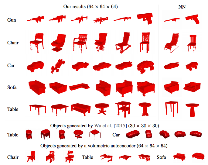
Qualitative results for 3D generated objects
For generation:
- Sample a 200-dimensional vector following an i.i.d. Uniform distr over [0,1]
- Render the largest connected component
Compare with
- 3D object synthesis from a probabilistic space [Wu et al., 2015]
- Volumetric auto-encoders (because latent space is not restricted, we fit a Gaussian to the empirical latent space distribution)
- Able to synthesize high-res 3D objects with detailed geometries
- Objects are similar, but not identical to training samples → not memorizing
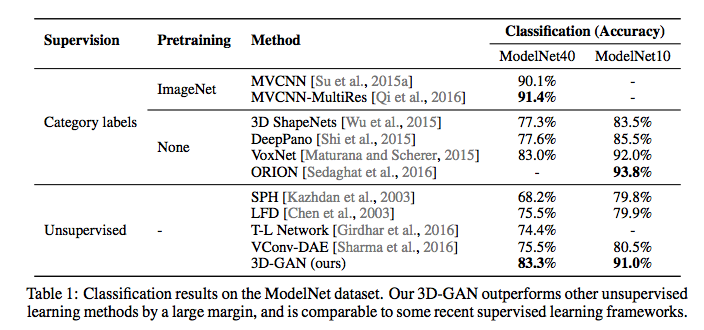
Classification performance of learned representations w/o supervision
Typical way to evaluate representations learned without supervision is to use them as features for classification. Input: 3D object Output: feature vector (concatenated the responses of the 2nd, 3rd, 4th convolutional layers in the discriminator, w/ applied max-pooling of size {8,4,2}) Classifier: Linear SVM
Train Data: ShapeNet Test Data: ModelNet {10, 40}
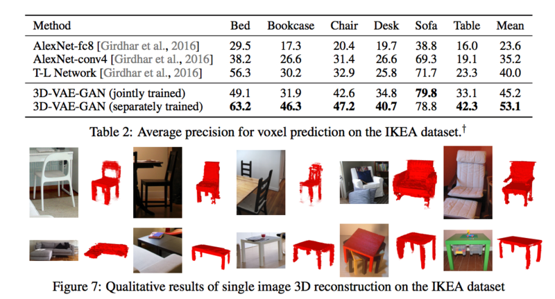
3D object reconstruction from a single image
Following previous work [Girdhar et al., 2016] the performance of 3D-VAE-GAN was evaluated on the IKEA dataset 1039 objects centre-cropped from 759 images (supplied by author) Images captured in the wild, often w/ cluttered backgrounds and occluded 6 categories: bed, bookcase, chair, desk, sofa, table Performance Single 3D-VAE-GAN trained on 6 categories Multiple 3D-VAE-GANs each trained on 1 category Align each prediction with GT over permutations, flips, and %10 translation
Analyzing learned representations for generator and discriminator
In this section we explore the learned representations of the generator and discriminator in a trained 3D-GAN. Starting with a $200$-dimensional vector as input, the generator neurons will fire to generate a 3D object, consequently leading to the firing of neurons in the discriminator which will produce a confidence value between $[0,1]$. To understand the latent space of vectors for object generation, we first vary the intensity of each dimension in the latent vector and observe the effect on the generated 3D objects. In Figure 5, each red region marks the voxels affected by changing values in a particular dimesnion of the latent vector. It can be seen that semantic meaning such as width and thickness of surfaces is encoded in each of these dimensions.
Next, we explore intra-class and inter-class object metamorphosis by interpolating between latent vector representation of a source and target 3D object. In Figure 6, we see a smooth transition exists for various types of chairs (w/ and w/o arm rests, and with varying backrest), as well as for a smooth transition between race car and speedboat.
Next, as is common in generative model evaluations, a simple arithmetic scheme is tested on latent vector representation of 3D objects. In Figure 8 shows that not only are generative networks able to encode semantic knowledge of chair and face images in its latent space, but these learned representations behave similarly as well. This can be seen because simple arithmetic on latent vector representations works in accord with intuition in Figure 8.
Finally, the authors explore the neurons in the discriminator. In order to understand firing patterns for specific neurons, the authors iterate through all training objects while keeping track of those samples that result in the highest firing intensity of a specific neuron. Here the neurons in the second-to-last convolutional layers were considered. From Figure 9, we conclude that neurons are selective: for a single neuron, the objects producing strongest activations are similar, and neurons learn semantics: the object parts that activate the neuron the most are consistent across objects.
Future Work and Open questions
Source
Wu, Zhirong, et al. ``3d shapenets: A deep representation for volumetric shapes. Proceedings of the IEEE Conference on Computer Vision and Pattern Recognition. 2015.
Chang, Angel X., et al. ``Shapenet: An information-rich 3d model repository. arXiv preprint arXiv:1512.03012 (2015).
<references />


