STAT946F17/ Improved Variational Inference with Inverse Autoregressive Flow: Difference between revisions
No edit summary |
|||
| Line 1: | Line 1: | ||
==Introduction== | ==Introduction== | ||
One of the most common ways to formalize machine learning models is through the use of $\textbf{latent variable models}$, wherein we have a probabilistic model for the joint distribution between observed datapoints $x$ and some $\textit{hidden variables}$. The intuition is that the hidden variables share some sort of (perhaps prolix) causal relationship with the variables that are actually observed. The $ \textbf{mixture of Gaussians}$ provides a particularly nice example of a latent variable model. One way to think about a mixture with $K$ Gaussians is as follows. First, roll a $K$-sided die and suppose that the result is $k$ with probabililty $\pi_{k}$. Then randomly generate a point from the Gaussian distribution with parameters $\mu_{k}$ and $\Sigma_{k}$. The reason this is a hidden variable model is that, when we have a dataset coming from a mixture of Gaussians, we only get to see the datapoints that are generated at the end. For a given observed datapoint we neither get to see the die that is rolled in generating that point nor do we know what the probabilities $\pi_{k}$ are. The $\pi_{k}$ are therefore hidden variables | One of the most common ways to formalize machine learning models is through the use of $\textbf{latent variable models}$, wherein we have a probabilistic model for the joint distribution between observed datapoints $x$ and some $\textit{hidden variables}$. The intuition is that the hidden variables share some sort of (perhaps prolix) causal relationship with the variables that are actually observed. The $ \textbf{mixture of Gaussians}$ provides a particularly nice example of a latent variable model. One way to think about a mixture with $K$ Gaussians is as follows. First, roll a $K$-sided die and suppose that the result is $k$ with probabililty $\pi_{k}$. Then randomly generate a point from the Gaussian distribution with parameters $\mu_{k}$ and $\Sigma_{k}$. The reason this is a hidden variable model is that, when we have a dataset coming from a mixture of Gaussians, we only get to see the datapoints that are generated at the end. For a given observed datapoint we neither get to see the die that is rolled in generating that point nor do we know what the probabilities $\pi_{k}$ are. The $\pi_{k}$ are therefore hidden variables. ML or MAP estimation for the parameters $\mu_{k}$, $\Sigma_{k}$ together with estimation of latent variables (i.e. $\pi_{k}$) given observations constitute inference within the mixture of Gaussians model. Note that all the parameters to be estimated can be wrapped into a long vector $\theta = (\pi_{1}, \ldots, \pi_{K}, \mu_{1}, \ldots \mu_{k}, \Sigma_{1}, \ldots, \Sigma_{K})$. | ||
More generally, latent variable models provide a powerful framework to mathematically encode a variety of phenomena which are naturally subject to stochasticity. Thus, they form an important part of the theory underlying many machine learning models. Indeed, it can even be said that most machine learning models, when viewed appropriately, are latent variable models. Therefore, it behoves us to obtain general methods which allow tractable inference within latent variable models. One such method is known as $\textbf{variational inference}$, which is a method in machine learning that approximates probability densities through optimization [David et al., 2017]. This method has been used in many applications and tends to be faster than classical methods, such as Markov chain Monte Carlo sampling. The idea behind this method is to first posit a family of densities and then to find the member of that family which is close to the target. Variational inference, in its modern form, was introduced to machine learning around two decades ago in the seminal paper [jordanVI]. More recently, and more apropos of deep learning, stochastic versions of variational inference are being combined with neural networks to provide robust estimation of parameters in probabilistic models. The original impetus for this fusion apparently stems from publication of [autoencoderKingma] and [autoencoderRezende]. In the interim, a cottage industry for application of stochastic variational inference or methods related to it have seemingly sprung up, especially as witnessed by the variety of autoencoders currently being sold at the bazaar. The paper [946paper] represents another interesting contribution in parameter estimation by way of deep learning. Note that, at time of writing, variational methods are being applied to a wide range of problems in machine learning and we will only develop the small part of it necessary for our purposes. But refer to [VISurvey] for a survey. | More generally, latent variable models provide a powerful framework to mathematically encode a variety of phenomena which are naturally subject to stochasticity. Thus, they form an important part of the theory underlying many machine learning models. Indeed, it can even be said that most machine learning models, when viewed appropriately, are latent variable models. Therefore, it behoves us to obtain general methods which allow tractable inference within latent variable models. One such method is known as $\textbf{variational inference}$, which is a method in machine learning that approximates probability densities through optimization [David et al., 2017]. This method has been used in many applications and tends to be faster than classical methods, such as Markov chain Monte Carlo sampling. The idea behind this method is to first posit a family of densities and then to find the member of that family which is close to the target. Variational inference, in its modern form, was introduced to machine learning around two decades ago in the seminal paper [jordanVI]. More recently, and more apropos of deep learning, stochastic versions of variational inference are being combined with neural networks to provide robust estimation of parameters in probabilistic models. The original impetus for this fusion apparently stems from publication of [autoencoderKingma] and [autoencoderRezende]. In the interim, a cottage industry for application of stochastic variational inference or methods related to it have seemingly sprung up, especially as witnessed by the variety of autoencoders currently being sold at the bazaar. The paper [946paper] represents another interesting contribution in parameter estimation by way of deep learning. Note that, at time of writing, variational methods are being applied to a wide range of problems in machine learning and we will only develop the small part of it necessary for our purposes. But refer to [VISurvey] for a survey. | ||
Revision as of 02:58, 29 October 2017
Introduction
One of the most common ways to formalize machine learning models is through the use of $\textbf{latent variable models}$, wherein we have a probabilistic model for the joint distribution between observed datapoints $x$ and some $\textit{hidden variables}$. The intuition is that the hidden variables share some sort of (perhaps prolix) causal relationship with the variables that are actually observed. The $ \textbf{mixture of Gaussians}$ provides a particularly nice example of a latent variable model. One way to think about a mixture with $K$ Gaussians is as follows. First, roll a $K$-sided die and suppose that the result is $k$ with probabililty $\pi_{k}$. Then randomly generate a point from the Gaussian distribution with parameters $\mu_{k}$ and $\Sigma_{k}$. The reason this is a hidden variable model is that, when we have a dataset coming from a mixture of Gaussians, we only get to see the datapoints that are generated at the end. For a given observed datapoint we neither get to see the die that is rolled in generating that point nor do we know what the probabilities $\pi_{k}$ are. The $\pi_{k}$ are therefore hidden variables. ML or MAP estimation for the parameters $\mu_{k}$, $\Sigma_{k}$ together with estimation of latent variables (i.e. $\pi_{k}$) given observations constitute inference within the mixture of Gaussians model. Note that all the parameters to be estimated can be wrapped into a long vector $\theta = (\pi_{1}, \ldots, \pi_{K}, \mu_{1}, \ldots \mu_{k}, \Sigma_{1}, \ldots, \Sigma_{K})$.
More generally, latent variable models provide a powerful framework to mathematically encode a variety of phenomena which are naturally subject to stochasticity. Thus, they form an important part of the theory underlying many machine learning models. Indeed, it can even be said that most machine learning models, when viewed appropriately, are latent variable models. Therefore, it behoves us to obtain general methods which allow tractable inference within latent variable models. One such method is known as $\textbf{variational inference}$, which is a method in machine learning that approximates probability densities through optimization [David et al., 2017]. This method has been used in many applications and tends to be faster than classical methods, such as Markov chain Monte Carlo sampling. The idea behind this method is to first posit a family of densities and then to find the member of that family which is close to the target. Variational inference, in its modern form, was introduced to machine learning around two decades ago in the seminal paper [jordanVI]. More recently, and more apropos of deep learning, stochastic versions of variational inference are being combined with neural networks to provide robust estimation of parameters in probabilistic models. The original impetus for this fusion apparently stems from publication of [autoencoderKingma] and [autoencoderRezende]. In the interim, a cottage industry for application of stochastic variational inference or methods related to it have seemingly sprung up, especially as witnessed by the variety of autoencoders currently being sold at the bazaar. The paper [946paper] represents another interesting contribution in parameter estimation by way of deep learning. Note that, at time of writing, variational methods are being applied to a wide range of problems in machine learning and we will only develop the small part of it necessary for our purposes. But refer to [VISurvey] for a survey.
Black-box Variational Inference
The basic premise we start from is that we have a latent variable model $p_{\theta}(x, h)$, often called the $\textbf{generative model}$ in the literature, with $x$ the observed variables and $h$ the hidden variables, and we wish to learn the parameters $\theta$. Hence, in variational inference, we are approximating the posterior $p_{\theta}(x, h)$ which has a variational distribution $q_{\phi}(h\mid x)$ with a motive to minimize the Kullback-Leibler divergence. Hence, we assume we are in a situation where the usual strategy of inference by maximum likelihood estimation is infeasible due to intractability of marginalization of the hidden variables. This assumption often holds in real-world applications since generative models for real phenomena are extremely difficult or impossible to integrate. Additionally, we would like to be able to compute the posterior $p(h\mid x)$ over hidden variables and, by Bayes' rule, this requires computation of the marginal distribution $p_{\theta}(x)$.
The variational inference approach entails positing a parametric family $q_{\phi}(h\mid x)$, also called the $\textbf{inference model}$, of distributions and introducing new learning parameters $\phi$ which obtain as solutions to an optimization problem. More precisely, we minimize the KL divergence between the true posterior and the approximate posterior. However, we can think of a slightly indirect approach. We can find a generic lower bound for the log-likelihood $\log p_{\theta}(x)$ and optimize for this lower bound. Observe that, for any parametrized distribution $q_{\phi}(h\mid x)$, we have \begin{align*} \log p_{\theta}(x) &= \log\int_{h}p_{\theta}(x,h) \\ &= \log\int_{h}p_{\theta}(x,h)\frac{q_{\phi}(h\mid x)}{q_{\phi}(h\mid x)} \\ &= \log\int_{h}\frac{p_{\theta}(x,h)}{q_{\phi}(h\mid x)}q_{\phi}(h\mid x) \\ &= \log\mathbb{E}_{q}\left[\frac{p_{\theta}(x,h)}{q_{\phi}(h\mid x)}\right] \\ &\geq \mathbb{E}_{q}\left[\log\frac{p_{\theta}(x,h)}{q_{\phi}(h\mid x)}\right] \end{align*}
Here we are trying to minimize the Kullback-Leibler which is achieved by maximizing the evidence lower bound:
\begin{align*} \log p_{\theta}(x) &= \mathbb{E}_{q}\left[\log p_{\theta}(x,h) - \log q_{\phi}(h\mid x)\right] \\ &:= \mathcal{L}(x, \theta, \phi), \end{align*}
where the inequality is an application of Jensen's inequality for the logarithm function and $\mathcal{L}(x,\theta,\phi)$ is known as the $\textbf{evidence lower bound (ELBO)}$. Clearly, if we iteratively choose values for $\theta$ and $\phi$ such that $\mathcal{L}(x,\theta,\phi)$ increases, then we will have found values for $\theta$ such that the log-likelihood $\log p_{\theta}(x)$ is non-decreasing (that is, there is no guarantee that a value for $\theta$ which increases $\mathcal{L}(x,\theta,\phi)$ will also increase $\log p_{\theta}(x)$ but there \textit{is} a guarantee that $\log p_{\theta}(x)$ will not decrease). The natural search strategy now is to use stochastic gradient ascent on $\mathcal{L}(x,\theta,\phi)$. This requires the derivatives $\nabla_{\theta}\mathcal{L}(x,\theta,\phi)$ and $\nabla_{\phi}\mathcal{L}(x,\theta,\phi)$.
Before moving on, we note that there are alternative ways of expressing the ELBO which can either provide insights or aid us in further calculations. For one alternative form, note that we can massage the ELBO like so. \begin{align*} \mathcal{L}(x, \theta, \phi) = & \mathbb{E}_{q} \left[ \log p_{\theta}(x, h) - \log q_{\phi}(h \mid x) \right] \\ = & \mathbb{E}_{q} \left[ \log p_{\theta}(h \mid x) p(x) - \log q_{\phi}(h \mid x) \right] \\ = & \mathbb{E}_{q} \left[ \log p_{\theta}(h \mid x) + \log p(x) - \log q_{\phi}(h \mid x) \right] \\ = & \mathbb{E}_{q} \left[ \log p(x) - \log q_{\phi}(h \mid x) + \log p_{\theta}(h \mid x) \right] \\ = & \mathbb{E}_{q} \left[ \log p(x) \right] - \mathbb{E}_{q} \left[ \log q_{\phi}(h \mid x) - \log p_{\theta}(h \mid x) \right] \\ = & \log p(x) - \mathrm{KL}\left[ q_{\phi}(h \mid x) || p(h \mid x) \right]. \end{align*} The last expression has a very simple interpretation: maximizing $\mathcal{L}(x, \theta, \phi)$ is equivalent to minimizing the KL divergence between the approximate posterior $q_{\phi}$ and the actual posterior $p_{\theta}(h \mid x)$. In fact, we can rewrite the above equation as a ``conservation law" \[ \mathcal{L}(x, \theta, \phi) + \mathrm{KL} \left[ q_{\phi}(h \mid x) || p(h \mid x) \right] = \log p(x). \] On the other hand, we can also do \begin{align*} \mathcal{L}(x, \theta, \phi) = & \mathbb{E}_{q} \left[ \log p_{\theta}(x, h) - \log q_{\phi}(h \mid x) \right] \\ = & \mathbb{E}_{q} \left[ \log p_{\theta}(x \mid h) p_{\theta}(h) - \log q_{\phi}(h \mid x) \right] \\ = & \mathbb{E}_{q} \left[ \log p_{\theta}(x \mid h) + \log p_{\theta}(h) - \log q_{\phi}(h \mid x) \right] \\ = & \mathbb{E}_{q} \left[ \log p_{\theta}(x \mid h) - \log q_{\phi}(h \mid x) + \log p_{\theta}(h) \right] \\ = & \mathbb{E}_{q} \left[ \log p_{\theta}(x \mid h) \right] - \mathrm{KL}\left[ q_{\phi}(h \mid x) || p_{\theta}(h) \right]. \end{align*} and the hermeneutics here is a bit more interesting. Recall that $q_{\phi}(h \mid x)$ is a distribution we get to choose and choosing a ``good" distribution means choosing something which we believe is faithful to the way observations get encoded or ``compressed" into ``hidden representations". Conversely, $p_{\theta}(x \mid h)$ may be thought as a decoder which unpacks latent ``codes" into observations. Thus, we can think of $\mathbb{E}_{q} \left[ \log p_{\theta}(x \mid h) \right]$ as the expected reconstruction error when we use $q_{\phi}$ as an encoder. The KL term is now interpreted as a regularizer which restricts divergence of the encoder from the prior distribution over latent codes. Note that these remarks simply provide an intuition and even though we use descriptors such as encoder and decoder, there is no \textit{a priori} reason to implement the distributions involved as encoder and decoder networks as in an autoencoder. Indeed, there is nothing preventing us from even letting $q_{\phi}$ compute an overcomplete feature representation $h$ of $x$ (i.e., dimensionality of $h$ is greater than that of $x$).
Regardless of which ELBO we use, inference requires the gradients of $\mathcal{L}(x, \theta, \phi)$. Notice that, no matter what, there are expectations with respect to $q_{\phi}$ involved and the presence of these expectations persists into the gradients. As an example, let us compute the gradients with the ELBO written as \[ \mathcal{L}(x, \theta, \phi) = \mathbb{E}_{q}\left[\log p_{\theta}(x,h) - \log q_{\phi}(h\mid x)\right]. \] The gradient with respect to $\theta$ is easy. \begin{align*} \nabla_{\theta}\mathcal{L}(x,\theta,\phi) &= \nabla_{\theta}\mathbb{E}_{q}\left[\log p_{\theta}(x,h) - \log q_{\phi}(h\mid x)\right] \\ &= \nabla_{\theta}\mathbb{E}_{q}\left[\log p_{\theta}(x,h)\right] - \nabla_{\theta}\mathbb{E}_{q}\left[\log q_{\phi}(h\mid x)\right] \\ &= \nabla_{\theta}\int_{h}\left[q_{\phi}(h\mid x)\log p_{\theta}(x,h)\right] \\ &= \int_{h}q_{\phi}(h\mid x)\nabla_{\theta}\log p_{\theta}(x,h) \\ &= \mathbb{E}_{q}\left[\nabla_{\theta}\log p_{\theta}(x,h)\right]. \end{align*} For the derivative with respect to the variational parameters $\phi$, we are going to exploit the identities $$\int_{h}\nabla_{\phi} q_{\phi}(h\mid x)=\nabla_{\phi}\int_{h}q_{\phi}(h\mid x)=\nabla_{\phi}1=0$$ and $$q_{\phi}(h\mid x)\nabla_{\phi}\log q_{\phi}(h\mid x)=\nabla_{\phi}q_{\phi}(h\mid x).$$ Note that the second identity will be used in a ``backwards" direction toward the end of the derivation below. We now have \begin{align*} \nabla_{\phi}\mathcal{L}(x, \theta, \phi) &= \nabla_{\phi}\mathbb{E}_{q}\left[\log p_{\theta}(x,h) -\log q_{\phi}(h\mid x)\right] \\ &= \nabla_{\phi}\mathbb{E}_{q}\left[\log p_{\theta}(x,h)\right] - \nabla_{\phi}\mathbb{E}_{q}\left[\log q_{\phi}(h\mid x)\right] \\ &= \nabla_{\phi}\int_{h}q_{\phi}(h\mid x)\log p_{\theta}(x,h) - \nabla_{\phi}\int_{h}q_{\phi}(h\mid x)\log q_{\phi}(h\mid x) \\ &= \int_{h}\log p_{\theta}(x,h)\nabla_{\phi}q_{\phi}(h\mid x) - \int_{h}\nabla_{\phi}q_{\phi}(h\mid x)\log q_{\phi}(h\mid x) \\ &= \int_{h}\log p_{\theta}(x,h)\nabla_{\phi}q_{\phi}(h\mid x) - \int_{h}\left(q_{\phi}(h\mid x)\frac{\nabla_{\phi}q_{\phi}(h\mid x)}{q_{\phi}(h\mid x)} + \log q_{\phi}(h\mid x)\nabla_{\phi}q_{\phi}(h\mid x) \right) \\ &= \int_{h}\log p_{\theta}(x,h)\nabla_{\phi}q_{\phi}(h\mid x) - \int_{h}\left(\nabla_{\phi}q_{\phi}(h\mid x) + \log q_{\phi}(h\mid x)\nabla_{\phi}q_{\phi}(h\mid x) \right) \\ &= \int_{h}\log p_{\theta}(x,h)\nabla_{\phi}q_{\phi}(h\mid x) - \int_{h}\nabla_{\phi}q_{\phi}(h\mid x) - \int_{h}\log q_{\phi}(h\mid x)\nabla_{\phi}q_{\phi}(h\mid x) \\ &= \int_{h}\log p_{\theta}(x,h)\nabla_{\phi}q_{\phi}(h\mid x) - 0 - \int_{h}\log q_{\phi}(h\mid x)\nabla_{\phi}q_{\phi}(h\mid x) \\ &= \int_{h}\left(\log p_{\theta}(x,h)\nabla_{\phi}q_{\phi}(h\mid x) - \log q_{\phi}(h\mid x)\nabla_{\phi}q_{\phi}(h\mid x) \right) \\ &= \int_{h}\left(\log p_{\theta}(x,h) - \log q_{\phi}(h\mid x)\right)\nabla_{\phi}q_{\phi}(h\mid x) \\ &= \int_{h}\left(\log p_{\theta}(x,h) - \log q_{\phi}(h\mid x)\right)q_{\phi}(h\mid x)\nabla_{\phi}\log q_{\phi}(h\mid x) \\ &= \mathbb{E}_{q}\left[\left(\log p_{\theta}(x,h) - \log q_{\phi}(h\mid x)\right)\nabla_{\phi}\log q_{\phi}(h\mid x)\right]. \end{align*}
Observe that everything we have done so far is completely general and independent of any specific modelling assumptions we may have had to make. Indeed, it is the model independence of this approach which led Ranganath et al. <ref name="bbvi"> Rajesh Ranganath, Sean Gerrish and David M. Blei. Black Box Variational Inference. Proceedings of the Seventeenth International Conference on Artificial Intelligence and Statistics, {AISTATS} 2014, Reykjavik, Iceland, April 22-25, 2014</ref> \cite{bbvi} to christen it $\textbf{black-box variational inference}$. The price we pay for such generality is that we have to calculate expectations against the distribution $q_{\phi}$. Broadly speaking, such expectations are intractable integrals for any approximate posterior approaching verisimilitude. However, the notion of $\textbf{normalizing flow}$ represents a technical innovation which allows use of flexible posteriors while maintaining tractability through calculation of expectations against simple distributions (e.g., Gaussians) only.
The Black-box Variational Inference framework actually can imply the expectation maximization algorithm, which is an iterative method to find maximum likelihood and maximum a posteriori in the statistical model with latent variables. It has been successful implementation on the problems like Gaussian mixture models.
Recalling the maximum likelihood is expressed as below. \[ \mathcal{L}(x,\theta,\phi) = \mathbb{E}_q [\log p_\theta(x \mid h)] - \mathrm{KL}[q_{\phi}(h \mid x) || p(h \mid x)] \] As mentioned before, we need to set $q_{\phi_k}(h\mid x) = p_{\theta_k}(h)$ to minimize the KL divergence with a given estimation of $\theta_k$. Then the maximization step is to calculate that \[ \mathcal{L}(x, \theta,\phi_k) = \mathbb{E}_{q_{\phi_k}} [\log p_{\theta}(x \mid h)] \]
And $\theta_{k+1}$ is updated in the maximization step as \[ \theta_{k+1} = argmax_{\theta} \mathbb{E}_{q_{\phi_k}}[\log p_{\theta}(x \mid h)] \]
Variational Inference using Normalizing Flows
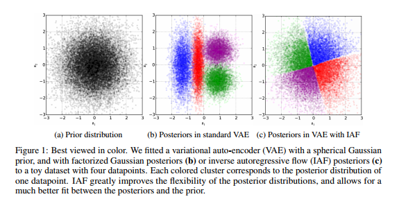
While our main goal is to describe \cite{946paper}, the paper \cite{normalizing_flow} provides the necessary conceptual backdrop for \cite{946paper} and we will now take a detour through some of the points presented in the latter. The main contribution of \cite{normalizing_flow} lies in a novel technique for creating a rich class of approximate posteriors starting from relatively simple ones. This is important since one of the main drawbacks to the variational approach is that it requires assumptions on the form of the approximate posterior $q_{\phi}(h\mid x)$ and practicality often forces us to stick to simple distributions which fail to capture rich, multimodal properties of the true posterior $p(h \mid x)$. The primary technical tool used in \cite{normalizing_flow} to achieve complexity in the approximate posterior is what we earlier referred to as normalizing flow, which entails using a series of invertible functions to transform simple probability densities into more complex densities.
Suppose we have a random variable $h$ with probability density $q(h)$ and that $f:\mathbb{R}^{d}\to\mathbb{R}^{d}$ is an invertible function with inverse $g:\mathbb{R}^{d}\to\mathbb{R}^{d}$. A basic result in probability states that the random variable $h'\colon = f(h)$ has distribution $$q'(h') = q(h)\Bigg\lvert\det\frac{\partial f}{\partial h}\Bigg\rvert^{-1}.$$ Chaining together a (finite) sequence of invertible maps $f_{1},\ldots,f_{K}$ and applying it to the distribution $q_{0}$ of a random variable $h_{0}$ leads to the formula $$q_{K}(h_{K}) = q_{0}(h_{0})\prod\limits^{K}_{k=1}\Bigg\lvert\det\frac{\partial f_{k}}{\partial h_{k-1}}\Bigg\rvert^{-1},$$ where $h_{k}\colon = f_{k}(h_{k-1})$ and $q_{k}$ is the distribution associated to $h_{k}$. We can equivalently rewrite the above equation as $$\log q_{K}(h_{K}) = \log q_{0}(h_{0}) - \sum\limits^{K}_{k=1}\log\Bigg\lvert\det\frac{\partial f_{k}}{\partial h_{k-1}}\Bigg\rvert.$$ So, if we were to start from a simple distribution $q_{0}(h_{0})$, choose a sequence of functions $f_{1},\ldots,f_{K}$ and then \textit{define} $$q_{\phi}(h \mid x)\colon = q_{K}(h_{K}),$$ we can manipulate the ELBO as follows: \begin{align*} \mathcal{L}(x,\theta,\phi) &= \mathbb{E}_{q}\left[\log p_{\theta}(x,h) - \log q_{\phi}(h\mid x)\right] \\ &= \mathbb{E}_{q_{K}}\left[\log p_{\theta}(x,h) - \log q_{K}(z_{K})\right] \\ &= \mathbb{E}_{q_{K}}\left[\log p_{\theta}(x,h)\right] - \mathbb{E}_{q_{K}}\left[\log q_{K}(z_{K})\right]. \end{align*} The reason this is an useful thing to do is the $\textbf{law of the unconscious statistician (LOTUS)}$ as applied to $q_{K} = f_{K}\circ\cdots\circ f_{1}(q_{0})$: $$\mathbb{E}_{q_{K}}\left[s(h_{K})\right] = \mathbb{E}_{q_{0}}\left[s(f_{K}\circ\cdots\circ f_{1}(h_{0}))\right]$$ assuming that $s$ does not depend on $q_{K}$. Hence, \begin{align*} \mathcal{L}(x,\theta,\phi) &= \mathbb{E}_{q_{K}}\left[\log p_{\theta}(x,h)\right] - \mathbb{E}_{q_{K}}\left[\log q_{K}(z_{K})\right] \\ &= \mathbb{E}_{q_{K}}\left[\log p_{\theta}(x,h)\right] - \mathbb{E}_{q_{K}}\left[\log q_{0}(h_{0}) - \sum\limits^{K}_{k=1}\log\Bigg\lvert\det\frac{\partial f_{k}}{\partial h_{k-1}}\Bigg\rvert\right] \\ &= \mathbb{E}_{q_{K}}\left[\log p_{\theta}(x,h)\right] - \mathbb{E}_{q_{K}}\left[\log q_{0}(h_{0})\right] - \mathbb{E}_{q_{K}}\left[\sum\limits^{K}_{k=1}\log\Bigg\lvert\det\frac{\partial f_{k}}{\partial h_{k-1}}\Bigg\rvert\right] \\ &= \mathbb{E}_{q_{0}}\left[\log p_{\theta}(x,h)\right] - \mathbb{E}_{q_{0}}\left[\log q_{0}(h_{0})\right] - \mathbb{E}_{q_{0}}\left[\sum\limits^{K}_{k=1}\log\Bigg\lvert\det\frac{\partial f_{k}}{\partial h_{k-1}}\Bigg\rvert\right] \end{align*} and we are only computing expectations with respect to the simple distribution $q_{0}$. The latter expression for ELBO is called the $\textbf{flow-based free energy bound}$ in \cite{normalizing_flow}. Note that $\theta$ has apparently disappeared in the final expression even though it is still present in $\mathcal{L}(x,\theta,\phi)$. This is an illusion: the parameters $\phi$ are associated to $q_{\phi}(h\mid x) = q_{K}(h_{K})$ and $q_{K}(h_{K})$ depends on the quantities $q_{0}(h_{0})$ and $\frac{\partial f_{k}}{\partial h_{k-1}}$. Thus, $\phi$ now encapsulates the defining parameters of $q_{0}$ and the $f_{k}$.
To summarize, we can start with a very simple distribution $q_{0}$ against which expectations are easy to calculate and if we can cleverly choose a series of invertible functions $\{f_{k}\}^{K}_{k=1}$ for which it is easy to compute determinants of the Jacobians, we can get a relatively rich approximate posterior $q_{K}$ such that the ELBO and its gradients are tractable. We should now ask: what is a suitable family of functions which can serve as a normalizing flow?
Inverse Autoregressive Flow
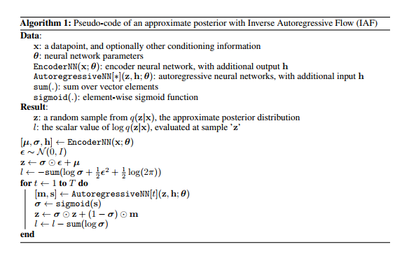
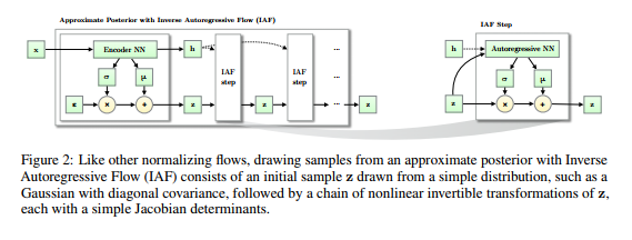
The answer presented by \cite{946paper} to the last question is \[ f_{k}(h_{k-1}) := \mu_{k} + \sigma_{k} \odot h_{k-1}, \] where $\odot$ means element-wise multiplication, $\mu_{k}$, $\sigma_{k}$ are outputs from an autoregressive neural network with inputs $h_{k-1}$ and an extra constant vector $c$ and we initialize with \[ h_{0} := \mu_{0} + \sigma_{0} \odot \epsilon \] such that $\epsilon \!\sim \mathcal{N}(0, I)$. The authors of \cite{946paper} call this series of functions the \textbf{inverse autoregressive flow}. We will solve the mystery of where this definition comes from later. The important point is that the functional form of $f_{k}$ is parametrized by the outputs of an autoregressive neural network and this implies that the Jacobians \[ \frac{\partial \mu_{k}}{\partial h_{k-1}}, \frac{\partial \sigma_{k}}{\partial h_{k-1}} \] are lower triangular with zeroes on the diagonal (this is not a trivial fact since $\mu_{k}$ and $\sigma_{k}$ are some complicated functions of $h_{k-1}$ -- they are outputs of a neural network which takes $h_{k-1}$ as an input). Hence, the derivative \[ \frac{\partial f_{k}}{\partial h_{k-1}} \] is a triangular matrix with the entries of $\sigma_{k}$ occupying the diagonal. The determinant of this is obviously just \[ \prod\limits^{D}_{i=1} \sigma_{k, i}, \] and it is very cheap to compute. Note also that the approximate posterior that comes out of this normalizing flow is \[ \log q_{K}(h_{K}) = - \sum\limits^{D}_{i=1} \left[ \frac{1}{2} \epsilon_{i}^{2} + \frac{1}{2} \log 2\pi + \sum\limits^{K}_{k=1} \log \sigma_{k,i} \right]. \] In conclusion, we have a nice expression for the ELBO. To round out the parsimony of the ELBO, we need an inference model which is computationally cheap to evaluate. Additionally, we typically do not calculate the ELBO gradients analytically but instead perform Monte Carlo estimation by sampling from the inference model. This requires inexpensive sampling from the inference model. Since expectations are calculated only with respect to the simple initial distribution $q_{0}$, both of these requirements are easily satisfied.
Inverse Autoregressive Transformations or, Whence Inverse Autoregressive Flow?
Once we have the inverse autoregressive flow, the main result of \cite{946paper} falls out. Let us consider how we could have come up with the idea of the inverse autoregressive flow. It will be helpful to start with a discussion of $\textbf{autoregressive neural networks}$, which we briefly alluded to when defining the flow. As the Latin prefix suggests, autoregression means that we deduce components of a random vector $h$ based on its \textit{own} components. More precisely, the $d^{th}$ element of $h$ depends on the preceding components $h_{1:d-1}$.
To elucidate this further, we shall follow the introductory exposition presented in \cite{MADE}. Let us consider a very simple autoencoder with just one hidden layer. That is, we have a feedforward neural network defined by \begin{align*} r(h) &:= g(b + Wh) \\ \hat{h} & := \mathrm{sigm}(c + Vr(h)), \end{align*} where $W$, $V$ are matrices of weights, $b$, $c$ are biases, $g$ is some non-linearity and $\mathrm{sigm}$ is element-wise sigmoid. Here, $r(h)$ is thought of as a hidden representation of the input $h$ and $\hat{h}$ is a reconstructed version of $h$. For simplicity, suppose that $h$ is a $D$-ary binary vector. Then we can measure the quality of our reconstruction using cross-entropy \[ l(h) := - \sum\limits h_{d} \log \hat{h}_{d} + (1 - h_{d}) \log (1 - \hat{h}_{d}). \] It is tempting to interpret $l(h)$ as a negative log-likelihood induced by the distribution \[ \prod\limits^{D}_{d=1} \hat{h}_{d}^{h_{d}} (1 - \hat{h}_{d})^{1 - h_{d}}. \] However, absent restrictions on the above expression, this is in general \textit{not} the case. As an example, suppose our hidden layer has as many units as the input layer. Then it is possible to drive the cross-entropy loss to $0$ by copying the input into the hidden layer. In this situation, $q(h) = 1$ for every possible $h$ and $q(h)$ is seen to actually not define a probability distribution.
If $l(h)$ is indeed to be a negative log-likelihood, i.e., \[ l(h) = - \log p(h) \] for a genuine probability distribution $p(h)$, it must satisfy \begin{align*} l(h) = & - \sum\limits^{D}_{d=1} \log p(h_{d} \mid h_{1:d-1}) \\ = & - \sum\limits^{D}_{d=1} h_{d} \log p(h_{d} = 1 \mid h_{1:d-1}) + (1 - h_{d}) \log p(h_{d} = 0 \mid h_{1:d-1}) \\ = & - \sum\limits^{D}_{d=1} h_{d} \log p(h_{d} = 1 \mid h_{1:d-1}) + (1 - h_{d})(1 - \log p(h_{d} = 1 \mid h_{1:d-1})). \end{align*} The first equation is just the chain rule of probability \[ p(h) = \prod\limits^{D}_{d=1} p(h_{d} \mid h_{1:d-1}), \] the second equation is true because of our assumption that each entry of $h$ is either $0$ or $1$ and the third equation holds due to the fact that $p(h)$ is a probability distribution. Comparing the naive cross-entropy loss \[ - \sum\limits h_{d} \log \hat{h}_{d} + (1 - h_{d}) \log (1 - \hat{h}_{d}) \] with the term \[ - \sum\limits^{D}_{d=1} h_{d} \log p(h_{d} = 1 \mid h_{1:d-1}) + (1 - h_{d})(1 - \log p(h_{d} = 1 \mid h_{1:d-1})), \] we see that a correct reconstruction (``correct" in the sense that the loss function is a negative log-likelihood) needs to satisfy \[ \hat{h}_{d} = \log p(h_{d} = 1 \mid h_{1:d-1}). \]
More generally, for a (deep) autoencoder we can require the reconstructed vector to have components satisfying \[ \hat{h}_{d} = p(h_{d} \mid h_{1:d-1}). \] In other words, the $d^{th}$ component is the probability of observing $h_{d}$ given the preceding components $h_{1:d-1}$. This latter property is known as the $\textbf{autoregressive property}$ since we can think of it as sequentially performing regression on the components of $h$. Unsurprisingly, an autoencoder satisfying the autoregressive property is called an $\textbf{autoregressive autoencoder}$.
Suppose now that we have an autoregressive autoencoder which takes an input vector $\mathbf{y} \in \mathbb{R}^{D}$ and we interpret the outputs of this network as parameters for a normal distribution. Write $[\mathbf{\mu}(\mathbf{y}),\mathbf{\sigma}(\mathbf{y})]$ for such output. The autoregressive structure implies that, for $j \in \{1, \ldots, D\}$, $\mathbf{y}_{j}$ depends only on the components $\mathbf{y}_{1:j-1}$. Therefore, if we take the vector $[\mathbf{\mu}_{i}, \mathbf{\sigma}_{i}]$ and compute the derivative with respect to $\mathbf{y}$, we will obtain a lower triangular matrix since \[ \frac{\partial [\mathbf{\mu}_{i}, \mathbf{\sigma}_{i}]}{\partial \mathbf{y}_{j}} = [0, 0] \] whenever $j \geq i$. We interpret the vector $[\mathbf{\mu}_{i}(\mathbf{y}_{1:j-1}), \mathbf{\sigma}_{i}(\mathbf{y}_{1:j-1})]$ as being the predicted mean and standard deviation of the $i^{th}$ element of (the reconstruction of) $\mathbf{y}$. In slightly more detail, the components of $\mathbf{y}$ are successively generated via \begin{align*} & \mathbf{y}_{0} = \mathbf{\mu}_{0} + \mathbf{\sigma}_{0} \cdot \mathbf{\epsilon}_{0}, \\ & \mathbf{y}_{i} = \mathbf{\mu}_{i}(\mathbf{y}_{1:i-1}) + \mathbf{\sigma}_{i}(\mathbf{y}_{1:i-1}) \cdot \mathbf{\epsilon}_{i}, \end{align*} where $\mathbf{\epsilon} \!\sim \mathcal{N}(\mathbf{0}, \mathbf{I})$.
To relate this back to the normalizing flow chosen by the authors of \cite{946paper}, replace $\mathbf{y}$ with $h_{k}$ as input to the autoregressive autoencoder and replace the outputs $\mathbf{\mu}$, $\mathbf{\sigma}$ with $\mu_{k}$, $\sigma_{k}$.
Implementation
The authors have open sourced the code for this paper on Github : https://github.com/openai/iaf
Experiments
The authors showcase the potential for improvement of variational autoencoders afforded by the novel IAF methodology they proposed by providing empirical evidence in the context of two key benchmark datasets: MNIST and CIFAR 10.
MNIST DATASET:
The results of the experiment authors conducted are displayed in the figure below. 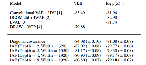
They provide some evidence as to the improvement of the variational inference via IAF when compared with other state of the art techniques.
CIFAR 10:
The results for the CIFAR 10 data set is displayed in the figure below. 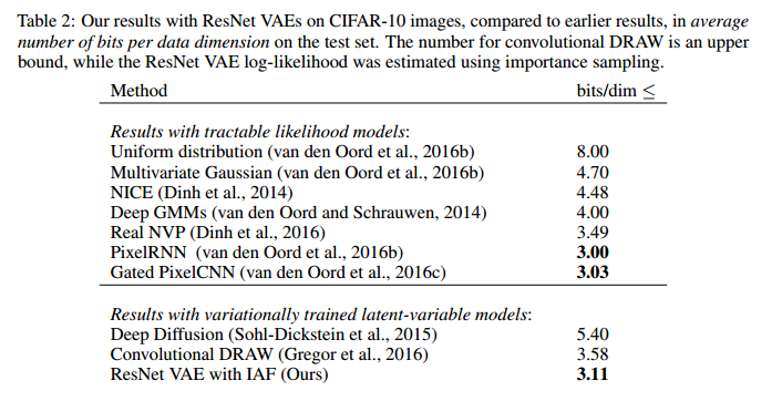
Concluding Remarks
In wrapping up, we note that there is something interesting about how the normalizing flow is derived. Essentially, the authors of \cite{946paper} took a neural network model with nice properties (fast sampling, simple Jacobian, etc.), looked at the function it implemented and basically dropped in this function in the recursive definition of the normalizing flow. This is not an isolated case. The authors of \cite{normalizing_flow} do much the same thing in coming up with the flow \[ f_{k}(h_{k}) = h_{k} + u_{k}s(w_{k}^{T}h_{k} + b_{k}). \] We believe that this flow is implicitly justified by the fact that functions of the above form are implemented by deep latent Gaussian models (see \cite{autoencoderRezende}). These flows, while interesting and useful, probably do not exhaust the possibilities for tractable and practical normalizing flows. It may be an interesting project to try and come up with novel normalizing flows by taking a favorite neural network architecture and using the function implemented by it as a flow. Additionally, it may be worth exploring boutique normalizing flows to improve variational inference in domain-specific settings (e.g., use a normalizing flow induced by a parsimonious convolutional neural network architecture for training an image-processing model using variational inference).
List of Figures
References
Blei, David M., Alp Kucukelbir, and Jon D. McAuliffe. "Variational inference: A review for statisticians." Journal of the American Statistical Association just-accepted (2017).
