STAT946F17/ Dance Dance Convolution

Methods

Pipeline:

1) extract an audio feature representation

2) feed the representation into a step placement algorithm estimating probabilities that a step lies within that frame

3) use a peak-picking process on the sequence of probabilities to identify the timestamps at which to place steps

4) given a sequence of timestamps, use a step selection algorithm to choose which steps to place at each time. Note the approach to this problem involves modeling the probability distribution $\mathbb{P}(m_n|m_{n-1},...,m_1)$, where $m_{n}$ is the $n^{th}$ step in the sequence.

Audio Representation

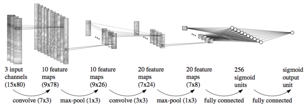
The final audio representation is a 15×80×3 tensor. These correspond to the temporal width of 15 representing 150ms of audio context, 80 frequency bands, and 3 different window lengths of 23ms, 46ms, and 93ms from short-time Fourier transform (STFT), where shorter window sizes preserve low-level features such as pitch and timbre while larger window sizes provide more context for high-level features such as melody and rhythm (Hamel et al., 2012)^[1]. Their approach to acoustic feature representation follows the work of Schlüter & Böck (2014)^[2], who develop similar representations to perform onset detection with CNNs. (Figure 5)

Figure 5: Network: 1)From the 3-channel spectrogram (corresponding to small, medium, large window sizes) excerpts of 15 frames by 80 bands 2)A convolutional layer with filters of 7 frames by 3 bands (by 3 channels) computes 10 feature maps of 9 frames by 78 bands. 3)Max-pooling over 3 adjacent bands without overlap, reducing the maps to 26 bands. 4)Another convolutional layer of 3×3 filters computes 20 feature maps of 7 frames by 24 bands. 5)Another 3-band max-pooling layer result in 20 maps of 7 frames by 8 bands (1120 neurons in total). 6)A fully-connected layer of 256 units 7)Applying the logistic sigmoid function, resulting in a single output unit with onset probability between 0.0 and 1.0

Step Placement

Models

• LSTM ^[3][4]

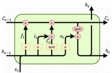
LSTM is able to handle sequences of any length and capture long-term dependencies

Figure 6: LSTM

$i_t = σ(W_i·[h_{t−1},x_t]+b_i)$

$f_t = σ(W_f·[h_{t−1},x_t]+b_f)$

$\tilde{c_t} = tanh(W_q·[h_{t−1},x_t]+b_q)$

$o_t = σ(W_o·[h_{t−1},x_t]+b_o)$

$c_t = f_t⊙c_{t−1}+i_t⊙\tilde{c_t}$

$h_t = o_t⊙tanh(c_t)$

where,

$i_t$: input gate, to control how much new information is going to be stored in the current memory cell.

$f_t$: forget gate, to control to what extent the information from the old memory cell is going to be thrown away.

$o_t$: output gate, to control what to output based on the memory cell $c_t$.

$h_{t-1}$: old hidden state

$x_t$: input at the current time step.

$c_t$: current memory cell

$σ$ is the logistic sigmoid function that has an output in [0, 1], $tanh$ denotes the hyperbolic tangent function that has an output in [−1, 1], and ⊙ denotes the elementwise multiplication.

• C-LSTM

Since CNN is able to learn trained features or, say, local response from temporal or spatial data but lacks the ability of learning sequential correlations; on the other hand, RNN(LSTM) is specialised for sequential modelling but unable to extract features in a parallel way. C-LSTM is created by proceeding LSTMs with a few fully connected CNN layers.

Figure 7: C-LSTM model used for step placement

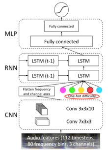
For step placement, all models considered have output consisting a single sigmoid unit which estimates the probability that a step is placed. Also, the authors augment the audio features with a one-hot representation of difficulty.

First, they use CNN model with the same structure as the CNN for onset detection (Figure 5) except for replacing 7) with another fully connected layer of 128 nodes.

Second the authors propose a C-LSTM model to improve upon the CNN by combining a convolutional encoding with an RNN that integrates information across longer windows of time. first apply two convolutional layers (of the same shape as the CNN) across the full unrolling length to encode the raw audio at each time step. The 3D tensor of the output is flattened along the channel and frequency axes (preserving the temporal dimension) and then the flattened features at each time step become the inputs to a two-layer RNN(LSTM). (Figure 7) LSTM consists of 2 layers with 200 nodes each. Two fully connected ReLU layers of dimension 256 and 128 are followed by the LSTM layers. The model is trained using 100 unrollings for backpropagation through time.

Note that a one-hot difficulty vector is added to improve the C-LSTM model. Since the paper does not show how it is added to the model, I modify the equations representing the operations of the LSTM cell to add the difficulty vector D to the input gate, forget gate, cell and output gate following the process of Ghosh 2016^[6].

$i_t = σ(W_i·[h_{t−1},x_t,D]+b_i)$

$f_t = σ(W_f·[h_{t−1},x_t,D]+b_f)$

$\tilde{c_t} = tanh(W_q·[h_{t−1},x_t,D]+b_q)$

$o_t = σ(W_o·[h_{t−1},x_t,D]+b_o)$

$c_t = f_t⊙c_{t−1}+i_t⊙\tilde{c_t}$

$h_t = o_t⊙tanh(c_t)$

Comparing the input gate equations before and after adding the difficulty vector D, we can see that having a difficulty vector D added into the CLSTM cell is equivalent to considering a composite input $[x_i\;D]$ to the LSTM cell that concatenates the original inputs and difficulty vectors.

Difficulty influences decisions about how many steps to place and where to place them. The average number of steps per second is less than one for low-difficulty charts, and more than seven steps per second for the highest-difficulty charts. Models are trained both with and without conditioning on difficulty, and found the inclusion of this feature to be informative.

Peak Picking

Figure 8: One second of peak picking. Green: Ground truth region (A):true positive, (B):false positive, (C):false negative, (D):two peaks smoothed to one by Hamming window, (E):misaligned peak accepted as true positive by ±20ms tolerance

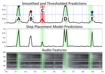
Following standard practice for onset detection, sequences of step probabilities are converted into a discrete set of chosen placements via a peak-picking process.

Steps:(Figure 8)

1) Running step placement algorithm over an entire song to assign the probabilities of a step occurring within each 10ms frame.

2) Convolving this sequence of predicted probabilities with a Hamming window, smoothing the predictions and suppressing double-peaks from occurring within a short distance.

3) Applying a constant threshold to choose which peaks are high enough.

References

1. Hamel, Philippe, Bengio, Yoshua, and Eck, Douglas. Building musically-relevant audio features through multiple timescale representations. In ISMIR, 2012.

2. Improved musical onset detection with CNN Schlüter & Böck (2014)

3. (Hochreiter and Schmidhuber, 1997)

4. A C-LSTM Neural Network for Text Classification

5. Convolutional, Long Short-Term Memory, Fully Connected Deep Neural Networks

6. Contextual LSTM (CLSTM) models for Large scale NLP tasks