One pixel attack for fooling deep neural networks

Presented by

1. Ziheng Chu

2. Minghao Lu

3. Qi Mai

4. Qici Tan

Introduction

Neural network first caught many people’s attention in imageNet contest in 2012. Neural network increased accuracy to 85% from 75%. The following year, it is increased to 89%. From no one used neural network to everyone uses the neural network. Today we have 97% accuracy in using deep neural network (DNN). So the problem of image recognition by are artificial intelligence is solved. However, there is one catch(Carlini.N,2017).

The catch is that the DNN is really easy to be fooled. Here is an example. An image of a dog is classified as a hummingbird. Research studies by Google Brian, which is a deep learning artificial intelligence research team at Google, showed that any machine learning classifier can be tricked to give wrong predictions. The action of designing an input in a specific way to get the wrong result from the model is called an adversarial attack (Roman Trusov,2017). The input image is the adversarial image. This image is created by adding a tiny amount of perturbation, which is not so imperceptible to human eyes. After zooming into figure 1, a small amount of perturbation led to misclassify a dog as a hummingbird.

Methodology

Problem Description

We can formalize the generation of adversarial images as an constrained optimization problem. We are given a classifier F and targeted adversarial class adv. Let x be the vectorized form of an image. Let F_adv(x) represent the probability assigned to the targeted class adv for vector x by the given classifier. Let e(x) represent an additive adversarial perturbation vector for image x. The goal of the targeted attack adversary is to find the perturbation vector with constrained size(norm) that maximizes the probability assigned to the targeted class by the classifier. Formally

For few-pixel attack, the problem statement is changed slightly. We constrain on the number of non-zero elements of the perturbation vector instead of the norm of the vector.

For the usual adversarial case, we can shift x in all dimensions, but the strength(norm) of the shift is bounded by L. For our one-pixel attack case, we are using the second equation with d=1. x is only allowed to be perturbed along a single axis, so the degree of freedom of the shift is greatly reduces. However, the shift in the one axis can be of arbitrary strength.

Differential Evolution

Differential evolution(DE) is a population based optimization algorithm belonging to the class of evolutionary algorithms(EA). For DE, in the selection process, the population is in a way "segmented" into families( offspring and parents ), and the most optimal from each family is chosen. This segmentation allows DE to keep more diversity in each iteration than other EAs and makes it more suitable for complex multi-modal optimization problems. Additionally, DE does not use gradient information, which makes it suitable for our problem.

Evaluation and Results

Measurement Metrics and Datasets

The authors used 4 measurement metrics to evaluate the effectiveness of the proposed attacks.

• Success Rate
  Non-targeted attack: the percentage of adversarial images were successfully classified to any possible classes other than the true one.
  

[math]\displaystyle{ \textrm{success rate }=\displaystyle\sum_{k=1}^N I(\textrm{Network}(\textrm{Attack}(\textrm{Image}_k))\neq \textrm{TrueClass}_k) }[/math]
Targeted attack: the probability of successfully classifying a perturbed image to a targeted class.

[math]\displaystyle{ \textrm{success rate }=\displaystyle\sum_{k=1}^N I(\textrm{Network}(\textrm{TargetedAttack}(\textrm{Image}_k))= \textrm{TrueClass}_k) }[/math]

• Adversarial Probability Labels (Confidence)
  The ratio of sum of probability level of the target class for each successful perturbation and the total number of successful attacks. This gives the mean confidence of the successful attacks on the target classification system.
• Number of Target Classes
  The number of images after perturbations cannot be classified to any other classes.
• Number of Original-Target Class Pairs
  The number of times of each pair being attacked.

Evaluation setups on CIFAR-10 test dataset:

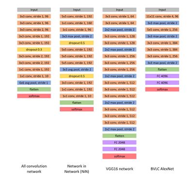
Three types of networks played as defense systems: All Convolutional Networks (AllConv), Network in Network (NiN) and VGG16 network. (See Figure 1)

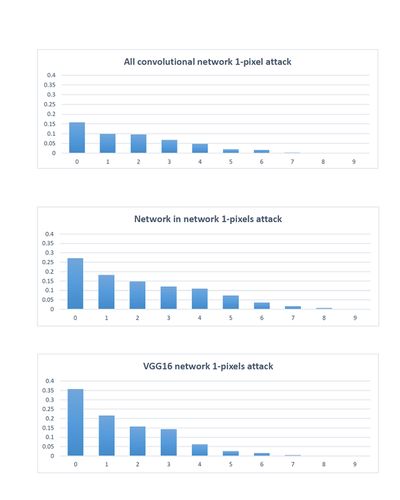
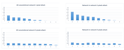
The authors randomly sampled 500 images, with resolution 32x32x3, from the dataset to perform one-pixel attacks and generated 500 samples with 3 and 5 pixel-modification respectively to conduct three-pixel and five-pixel attacks. The effectiveness of one-pixel attack was evaluated on all three introduced networks and the performance comparison, using success rate, was performed as the following: 1-pixel attack and 3-pixel attack on AllConv and 5-pixel attack on NiN.

Both targeted attacks and non-targeted attacks were considered but only targeted attacks were conducted since the performance of non-targeted attack results could be obtained from the result of targeted attacks by applying a fitness function to increase the probability level of the target class.

Evaluation setups on ImageNet validation dataset (ILSVRC 2012):

BVLC AlexNet played as defense system. (See Figure 1)

600 sample images were randomly sampled from the dataset. Due to the relatively high resolution of the images (224x224x3), only one-pixel attacked was carried out aiming to verify if extremely small pixel modification in a relatively large image can alternate the classification result.

Since the number of classes in this dataset is way larger than the one of CIFAR-10, the authors only launched non-targeted attacks and applied a fitness function to decrease the probability level of the true class.

Figure 1. Networks Architecture

Results

Figure 2. One-pixel attack on three networks (Su, Vargas and Sakurai, 2018)

Figure 3. 1, 3 and 5-pixel attacks (Su, Vargas and Sakurai, 2018)