learning Convolutional Feature Hierarchies for Visual Recognition
Overview
This paper<ref>Kavukcuoglu, K, Sermanet, P, Boureau, Y, Gregor, K, Mathieu, M, and Cun, Y. . Learning convolutional feature hierarchies for visual recognition. In Advances in neural information processing systems, 1090-1098, 2010.</ref> describes methods for learning features extracted through convolutional feature banks. In particular, it gives methods for using sparse coding convolutionally. This paper proposed to improve the feature extraction efficiency by jointly learning a feed-forward encoder with the convolutional filter bank, and applied the algorithm to Convolutional Networks (ConvNets), achieving impressive results on object recognition. In fact, Natural images, sounds, and more generally, signals that display translation invariance in any dimension, are better represented using convolutional dictionaries. sparse coding typically assumes that training image patches are independent from each other, and thus neglects the spatial correlation among them. In sparse coding, the sparse feature vector z is constructed to reconstruct the input x with a dictionary D. The procedure produces a code z* by minimizing the energy function:
- [math]\displaystyle{ L(x,z,D) = \frac{1}{2}||x-Dz||_2^2 + |z|_1, \ \ \ z^* = \underset{z}{\operatorname{arg\ min}} \ L(x,z,D) }[/math]
D is obtained by minimizing the above with respect to D: [math]\displaystyle{ \underset{z,D}{\operatorname{arg\ min}} \ L(x,z,D) }[/math], averaged over the training set. The drawbacks to this method are that the representation is redundant and that the inference for a whole image is computationally expensive. The reason is that the system is trained on single image patches in most applications of sparse coding to image analysis, which produces a dictionary of filters that are essentially shifted versions of each other over the patch and reconstructed in isolation.
This first problem can be addressed by applying sparse coding to the entire image and treating the dictionary as a convolutional filter bank. Invariance is classically achieved by regularization of the latent representation, e.g., by enforcing sparsity.
- [math]\displaystyle{ L(x,z,D) = \frac{1}{2}||x - \sum_{k=1}^K D_k * z_k ||_2^2 + |z|_1 }[/math]
Where Dk is an s×s filter kernel, x is a w×h image, zk is a feature map of dimension (w+s-1)×(h+s-1), and * denotes the discrete convolution operator.
The second problem can be addressed by using a trainable feed-forward encoder to approximate the sparse code:
- [math]\displaystyle{ L(z,z,D,W) = \frac{1}{2}||x - \sum_{k=1}^K D_k * z_k ||_2^2 + \sum_{k=1}^K||z_k - f(W^k*x)||_2^2 + |z|_1, \ \ \ z^* = \underset{z}{\operatorname{arg\ max}} \ L(x,z,D,W) }[/math]
Where Wk is an encoding convolutional kernel of size s×s, and f is a point-wise non-linear function. Both the form of f and the method to find z* are discussed below. Here, they used feed-forward neural networks to approximate sparse codes generated by sparse coding and avoided solving computationally costly optimizations at runtime.
The contribution of this paper is to address these two issues simultaneously, thus allowing convolutional approaches to sparse coding.
Method
The authors extend the coordinate descent sparse coding algorithm detailed in <ref>Li, Y and Osher, S. Coordinate Descent Optimization for l1 Minimization with Application to Compressed Sensing; a Greedy Algorithm. CAM Report, pages 09–17.</ref> to use convolutional methods.
Two considerations for learning convolution dictionaries are:
- Boundary effects due to convolution must be handled.
- Derivatives should be calculated efficiently.
function ConvCoD[math]\displaystyle{ \, (x,D,\alpha) }[/math]
- Set: [math]\displaystyle{ \, S = D^T*D }[/math]
- Initalize: [math]\displaystyle{ \, z = 0;\ \beta = D^T * mask(x) }[/math]
- Require: [math]\displaystyle{ \, h_\alpha: }[/math]: smooth thresholding function
- repeat
- [math]\displaystyle{ \, \bar{x} = h_\alpha(\beta) }[/math]
- [math]\displaystyle{ \, (k,p,q) = \underset{i,m,n}{\operatorname{arg\ max}} |z_{imn}-\bar{z_{imn}}| }[/math] (k: dictionary index, (p,q) location index)
- [math]\displaystyle{ \, bi = \beta_{kpq} }[/math]
- [math]\displaystyle{ \, \beta = \beta + (z_kpg - \bar{z_{kpg}}) \times align(S(:,k,:,:),(p,q)) }[/math] **
- [math]\displaystyle{ \, z_{kpg} = \bar{z_{kpg}},\ \beta_{kpg} = bi }[/math]
- until change in [math]\displaystyle{ z }[/math] is below a threshold
- end function
** MATLAB notation is used for slicing the tensor.
The second important point in training convolutional dictionaries is the computation of the S = [math]\displaystyle{ D_{T}^T ∗ D }[/math] operator. For most algorithms like coordinate descent , FISTA and matching pursuit [12], it is advantageous to store the similarity matrix (S) explicitly and use a si128 convolutional filters (W) learned in the encoder using smooth shrinkage function. ngle column at a time for updating the corresponding component of code z. For convolutional modeling, the same approach can be followed with some additional care. In patch based sparse coding, each element [math]\displaystyle{ (i, j) }[/math] of S equals the dot product of dictionary elements i and j. Si128 convolutional filters (W) learned in the encoder using smooth shrinkage function. 128 convolutional filters (W) learned in the encoder using smooth shrinkage function. nce the similarity of a pair of dictionary elements has to be also considered in spatial dimensions, each term is expanded as “full” convolution of two dictionary elements [math]\displaystyle{ (i, j) }[/math], producing [math]\displaystyle{ 2s−1×2s−1 }[/math] matrix. It is more convenient to think about the resulting matrix as a 4D tensor of size [math]\displaystyle{ K × K × 2s − 1 × 2s − 1 }[/math]. One should note that, depending on the input image size, proper alignment of corresponding column of this tensor has to be applied in the z space. One can also use the steepest descent algorithm for finding the solution to convolutional sparse coding given in equation 2, however using this method would be orders of magnitude slower compared to specialized algorithms like CoD and the solution would never contain exact zeros. In algorithm 1 we explain the extension of the coordinate descent algorithm for convolutional inputs. Having formulated convolutional sparse coding, the overall learning procedure is simple stochastic (online) gradient descent over dictionary D: In the above, [math]\displaystyle{ \beta = D^T * mask(x) }[/math] is use to handle boundary effects, where mask operates term by term and either puts zeros or scales down the boundaries.
The learning procedure is then stochastic gradient descent over the dictionary D, where the columns of D are normalized after each iteration.
- [math]\displaystyle{ \forall x^i \in X }[/math] training set: [math]\displaystyle{ z* = \underset{z}{\operatorname{arg\ max}}\ L(x^i,z,d), D \leftarrow D - \eta \frac {\partial(L,x^i,z^*,D}{\partial D} }[/math]
Two encoder architectures are tested. The first is steepest descent sparse coding with tanh encoding function using [math]\displaystyle{ g^k \times tanh(x*W^k) }[/math], which does not include a shrinkage operator. Thus the ability to produce sparse representations is very limited.
The second is convolutional CoD sparse coding with a smooth shrinkage operator as defined below.
- [math]\displaystyle{ \tilde{z}=sh_{\beta^k,b^k}(x*W^k) }[/math] where k = 1..K.
- [math]\displaystyle{ sh_{\beta^k,b^k}(s) = sign(s) \times 1/\beta^k \log(\exp(\beta^k \times |s|) - 1) - b^k }[/math]
where [math]\displaystyle{ \beta }[/math] controls the smoothness of the kink of shrinkage operator and b controls the location of the kink. The second system in more efficient in training, but the performance for both systems are almost identical.
The following figure shows the Smooth shrinkage function, : Total loss as a function of number of iterat128 convolutional filters (W) learned in the encoder using smooth shrinkage function. ions and 128 convolutional filters (W) learned in the encoder using smooth shrinkage function.
The convolutional encoder can also be used in multi-stage object recognition architectures. For each stage, the encoder is followed by absolute value rectification, contrast normalization and average subsampling.
Experiments
Two systems are used:
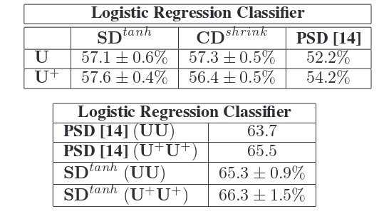
- Steepest descent sparse coding with tanh encoder: [math]\displaystyle{ SD^{tanh} }[/math]
- Coordinate descent sparse coding with shrink encoder: [math]\displaystyle{ CD^{shrink} }[/math]
Object Recognition using Caltech-101 Dataset
In the Caltech-101 dataset, each image contains a single object. Each image is processed by converting to grayscale and resizing, followed by contrast normalization. All results use 30 training samples per class and 5 different choices of the training set.
Architecture: 64 features are extracted by the first layer, followed by a second layer that produces 256 features. Second layer features are connected to first layer features by a sparse connection table.
First Layer: Both systems are trained using 64 dictionary elements, where each dictionary item is a 9×9 convolution kernel. Both systems are trained for 10 sparsity values from 0.1-3.0.
Second Layer: In the second layer, each of 256 feature maps in connected to 16 randomly selected input features from the first layer.
One Stage System: In these results, the input is passed to the first layer, followed by absolute value rectification, contrast normalization, and average pooling. The output of the first layer is fed to a logistic classifier followed by the PMK-SVN classifier used in <ref>Lazebnik, S, Schmid, C, and Ponce, J. Beyond bags of features: Spatial pyramid matching for recognizing natural scene categories. CVPR’06, 2:2169–2178, 2006.</ref>.
Two Stage System: These results use both layers, followed by absolute value rectification, contrast normalization, and average pooling. Finally, a multinomial logistic regression classifier is used.
In the above, U represents one stage, UU represents two stages, and '+' represents supervised training is performed afterwards. Each row of filters connect a particular second layer feature map. It is seen that each row of filters extract similar features since their output response is summed together to form one output feature map.
The following filters show the second stage filters. On the left, the Encoder kernels that correspond to the dictionary elements. On the right, the 128 dictionary elements, each row shows 16 dictionary elements, connecting to a single second layer feature map. It can be seen that each group extracts similar type of features from their corresponding inputs.
Pedestrian Detection
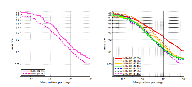
The architecture is trained and evaluated on the INRIA Pedestrian dataset <ref>Dalal, N and Triggs, B. Histograms of oriented gradients for human detection. In Schmid, C, Soatto, S, and Tomasi, C, editors, CVPR’05, volume 2, pages 886–893, June 2005.</ref> which contains 2416 positive examples (after mirroring) and 1218 negative full images. For training, the dataset is augmented with minor translations and scaling, giving a total of 11370 examples for training and 1000 images for classification. The negative examples are augmented with larger scale variations to avoid false positives, giving a total of 9001 samples for training and 1000 for validation.
The architecture for the pedestrian detection task is similar to that described in the previous section. It was trained both with and without unsupervised initialization, followed by supervised training. After one pass of training, the negative set was augmented with the 10 most offending samples on each full negative image.
Discussion
- The paper presented an efficient method for convolutional training of feature extractors.
- The resulting features look intuitively better than those obtained through non-convolutional methods, but classification results are only slightly better (where they're better at all) than existing methods.
- It's not clear what effects in the pedestrian experiment are due to the method of preprocessing and variations on the dataset (scaling and translation) and which are due to the architecture itself. Comparisons are with other systems that processed input differently.
- Unsupervised learning significantly helps to properly model extensive
variations in the dataset where a pure supervised learning algorithm fails
References
<references />


