joint training of a convolutional network and a graphical model for human pose estimation
Introduction
Human body pose estimation, or specifically the localization of human joints in monocular RGB images, remains a very challenging task in computer vision. Recent approaches to this problem fall into two broad categories: traditional deformable part models and deep-learning based discriminative models. Traditional models rely on the aggregation of hand-crafted low-level features and then use a standard classifier or a higher level generative model to detect the pose, which require the features to be sensitive enough and invariant to deformations. Deep learning approaches learn an empirical set of low and high-level features which are more tolerant to variations. However, it’s difficult to incorporate prior knowledge about the structure of the human body.
This paper proposes a new hybrid architecture that consists of a deep Convolutional Network Part-Detector and a part-based Spatial-Model. In other words, a deep convolutional neural network is combined with a graphical models, in order to capture the spatial dependencies between the variables of interest which is done using a joint-training process. This combination and joint training significantly outperforms existing state-of-the-art models on the task of human body pose recognition.
Model
Convolutional Network Part-Detector
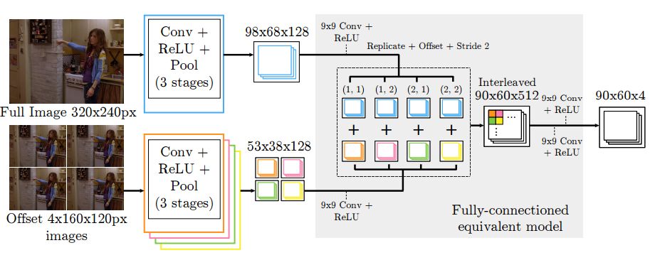
They combine an efficient ConvNet architecture with multi-resolution and overlapping receptive fields, which is shown in the figure below.
Traditionally, in image processing tasks such as these, a Laplacian Pyramid<ref> "Pyramid (image processing)" </ref> of three resolution banks is used to provide each bank with non-overlapping spectral content. Then the Local Contrast Normalization (LCN<ref> Collobert R, Kavukcuoglu K, Farabet C.Torch7: A matlab-like environment for machine learning BigLearn, NIPS Workshop. 2011 (EPFL-CONF-192376). </ref>) is applied to those input images. However, in this model, only a full image stage and a half-resolution stage was used, allowing for a simpler architecture and faster training.
Although, a sliding window architecture is usually used for this type of task, it has the down side of creating redundant convolutions. Instead, in this network, for each resolution bank, ConvNet architecture with overlapping receptive fields is used to get a heat-map as output, which produces a per-pixel likelihood for key joint locations on the human skeleton.
The following figure shows a Efficient Sliding Window Model with Overlapping Receptive Fields,

The convolution results (feature maps) of the low resolution bank are upscaled and interleaved with those of high resolution bank. Then, these dense feature maps are processed through convolution stages at each pixel, which is equivalent to fully-connected network model but more efficient.
Supervised training of the network is performed using batched Stochastic Gradient Descent (SGD) with Nesterov Momentum.
Nesterov momentum can be written as<ref> Ilya Sutskever, James Martens, George E. Dahl, and Geoffrey E. Hinton. On the importance of initialization and momentum in deep learning. In Proceedings of the 30th International Conference on Machine Learning, ICML 2013, Atlanta, GA, USA, 16-21 June 2013, volume 28 of JMLR Proceedings, pages 1139–1147. JMLR.org, 2013. </ref>:
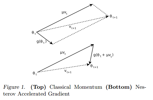
Rather than adding each set of gradients from the stochastic batch process separately, a velocity vector is instead accumulated at some rate [math]\displaystyle{ \,\mu }[/math] so that if the gradient descent process continuously travel in the same general direction, then this velocity vector would increase over each successive descent and travel faster towards that direction than conventional gradient descent. This should increase the convergence rate and decrease number of epochs needed to converge to some local minima. Nesterov momentum does make one modification and that is to correct the direction of the velocity vector with [math]\displaystyle{ \,\epsilon\triangledown f(\theta_t+\mu v_t) }[/math] not at the current position, but at the future predicted position. The difference can be seen in the figure<ref> Ilya Sutskever, James Martens, George E. Dahl, and Geoffrey E. Hinton. On the importance of initialization and momentum in deep learning. In Proceedings of the 30th International Conference on Machine Learning, ICML 2013, Atlanta, GA, USA, 16-21 June 2013, volume 28 of JMLR Proceedings, pages 1139–1147. JMLR.org, 2013. </ref>:
This correction lets the descent direction be more sensitive to changes in directions and increases stability. This can be seen as looking at the future gradient to evaluate the suitability of the current gradient direction. This is evident in the figure where the first changes direction based purely at the current position and the second corrects the direction based on the next gradient.
They use a Mean Squared Error (MSE) criterion to minimize the distance between the predicted output and a target heat-map. At training time they also perform random perturbations of the input images (randomly flipping and scaling the images) to increase generalization performance.
Higher-Level Spatial-Model
They use a higher-level Spatial-Model to get rid of false positive outliers and anatomically incorrect poses predicted by the Part-Detector, constraining joint inter-connectivity and enforcing global pose consistency.
They formulate the Spatial-Model as an Markov Random Field (MRF)-like model over the distribution of spatial locations for each body part. MRFs are undirected probabilistic graphical models; a conditional-independence structure not enforcing directionality in dependence relations between variables. After the unary potentials for each body part location are provided by the Part-Detector, the pair-wise potentials in the graph are computed using convolutional priors, which model the conditional distribution of the location of one body part to another. For instance, the final marginal likelihood for a body part A can be calculated as:
[math]\displaystyle{ \bar{p}_{A}=\frac{1}{Z}\prod_{v\in V}^{ }\left ( p_{A|v}*p_{v}+b_{v\rightarrow A} \right ) }[/math]
Where [math]\displaystyle{ v }[/math] is the joint location, [math]\displaystyle{ p_{A|v} }[/math] is the conditional prior which is the likelihood of the body part A occurring in pixel location (i, j) when joint [math]\displaystyle{ v }[/math] is located at the center pixel, [math]\displaystyle{ b_{v\rightarrow A} }[/math] is a bias term used to describe the background probability for the message from joint [math]\displaystyle{ v }[/math] to A, and Z is the partition function. The learned pair-wise distributions are purely uniform when any pairwise edge should be removed from the graph structure. The above equation is analogous to a single round of sum-product belief propagation. Convergence to a global optimum is not guaranteed given that this spatial model is not tree structured. However, the inferred solution is sufficiently accurate for all poses in datasets used in this research.
For their practical implementation, they treat the distributions above as energies to avoid the evaluation of Z in the equation before. Their final model is
[math]\displaystyle{ \bar{e}_{A}=\mathrm{exp}\left ( \sum_{v\in V}^{ }\left [ \mathrm{log}\left ( \mathrm{SoftPlus}\left ( e_{A|v} \right )*\mathrm{ReLU}\left ( e_{v} \right )+\mathrm{SoftPlus}\left ( b_{v\rightarrow A} \right ) \right ) \right ] \right ) }[/math]
[math]\displaystyle{ \mathrm{where:SoftPlus}\left ( x \right )=\frac{1}{\beta }\mathrm{log}\left ( 1+\mathrm{exp}\left ( \beta x \right ) \right ), 0.5\leq \beta \leq 2 }[/math]
[math]\displaystyle{ \mathrm{ReLU}\left ( x \right )=\mathrm{max}\left ( x,\epsilon \right ), 0\lt \epsilon \leq 0.01 }[/math]
This model replaces the outer multiplication of final marginal likelihood with a log space addition to improve numerical stability and to prevent coupling of the convolution output gradients (the addition in log space means that the partial derivative of the loss function with respect to the convolution output is not dependent on the output of any other stages).
With this modified formulation, the equation can be trained by using back-propagation and SGD. The network-based implementation of the equation is shown below.
The convolution sizes are adjusted so that the largest joint displacement is covered within the convolution window. For the 90x60 pixel heat-map output, this results in large 128x128 convolution kernels to account for a joint displacement radius of 64 pixels (padding is added on the heat-map input to prevent pixel loss). The convolution kernels they use in this step is quite large, thus they apply FFT convolutions based on the GPU, which is introduced by Mathieu et al.<ref> Mathieu M, Henaff M, LeCun Y.Fast training of convolutional networks through ffts arXiv preprint arXiv:1312.5851, 2013. </ref>.The convolution weights are initialized using the empirical histogram of joint displacements created from the training examples. Moreover, during training they randomly flip and scale the heat-map inputs to improve generalization performance.The motivation for this approach is that using multiple scales may help capturing contextual information.
Unified Model
They first train the Part-Detector separately and store the heat-map outputs, then use these heat-maps to train a Spatial-Model. Finally, they combine the trained Part-Detector and Spatial-Models and back-propagate through the entire network, which further improves performance. Because the SpatialModel is able to effectively reduce the output dimension of possible heat-map activations, the PartDetector can use available learning capacity to better localize the precise target activation.
Results
They evaluated their architecture on the FLIC and extended-LSP datasets. The FLIC dataset is comprised of 5003 images from Hollywood movies with actors in predominantly front-facing standing up poses, while the extended-LSP dataset contains a wider variety of poses of athletes playing sport. They also proposed a new dataset called FLIC-plus<ref> "FLIC-plus Dataset" </ref> which is fairer than FLIC-full dataset.
Their model’s performance on the FLIC test-set for the elbow and wrist joints is shown below. It’s trained by using both the FLIC and FLIC-plus training sets.
Performance on the LSP dataset is shown here.
Since the LSP dataset cover a larger range of the possible poses, their Spatial-Model is less effective. The accuracy for this dataset is lower than FLIC. They believe that increasing the size of the training set will improve performance for these difficult cases.
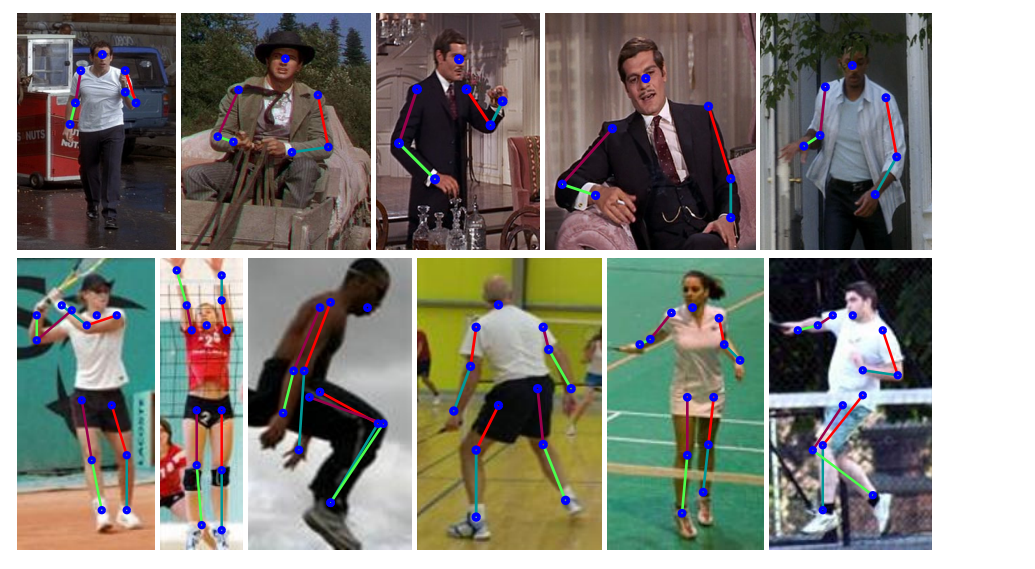
The following figure shows the predicted joint locations for a variety of inputs in the FLIC and LSP test-sets. The network produces convincing results on the FLIC dataset (with low joint position error), however, because the simple Spatial-Model is less effective for a number of the highly articulated poses in the LSP dataset, the detector results in incorrect joint predictions for some images. Increasing the size of the training set will improve performance for these difficult cases.

Conclusion
In this paper a one step message passing is implemented as a convolution operation in order to incorporate spatial relationship between local detection responses for human body pose estimation.This paper shows that the unification of a novel ConvNet Part-Detector and an MRF inspired SpatialModel into a single learning framework significantly outperforms existing architectures on the task of human body pose recognition. Training and inference of the architecture uses commodity level hardware and runs at close to real-time frame rates, making this technique tractable for a wide variety of application areas.
Bibliography
<references />

