Influenza Forecasting Framework based on Gaussian Processes
Abstract
This paper presents a novel framework for seasonal epidemic forecasting using Gaussian process regression. Resulting retrospective forecasts, trained on a subset of the publicly available CDC influenza-like-illness (ILI) data-set, outperformed four state-of-the-art models when compared using the official CDC scoring rule (log-score).
Background
Each year, the seasonal influenza epidemic affects public health at a massive scale, resulting in 38 million cases, 400 000 hospitalizations, and 22 000 deaths in the United States in 2019/20 alone (cite CDC). Given this, reliable forecasts of future influenza development are invaluable, because they allow for improved public health policies and informed resource development and allocation.
Related Work
Given the value of epidemic forecasts, the CDC regularly publishes ILI data and has funded a seasonal ILI forecasting challenge. This challenge has lead to four state of the art models in the field; MSS, a physical susceptible-infected-recovered model with assumed linear noise; SARIMA, a framework based on seasonal auto-regressive moving average models; and LinEns, an ensemble of three linear regression models.
Motivation
It has been shown that LinEns forecasts outperform the other frameworks on the ILI data-set. However, this framework assumes a deterministic relationship between the epidemic week and its case count, which does not reflect the stochastic nature of the trend. Therefore, it is natural to ask whether a similar framework that assumes a stochastic relationship between these variables would provide better performance. This motivated the development of the proposed Gaussian process regression framework, and the subsequent performance comparison to the benchmark models.
Gaussian Process Regression
Consider the following set up: let [math]\displaystyle{ X = [\mathbf{x}_1,\ldots,\mathbf{x}_n] }[/math] [math]\displaystyle{ (d\times n) }[/math] be your training data, [math]\displaystyle{ \mathbf{y} = [y_1,y_2,\ldots,y_n]^T }[/math] be your noisy observations where [math]\displaystyle{ y_i = f(\mathbf{x}_i) + \epsilon_i }[/math], [math]\displaystyle{ (\epsilon_i:i = 1,\ldots,n) }[/math] i.i.d. [math]\displaystyle{ \sim \mathcal{N}(0,{\sigma}^2) }[/math], and [math]\displaystyle{ f }[/math] is the trend we are trying to model (by [math]\displaystyle{ \hat{f} }[/math]). Let [math]\displaystyle{ \mathbf{x}^* }[/math] [math]\displaystyle{ (d\times 1) }[/math] be your test data point, and [math]\displaystyle{ \hat{y} = \hat{f}(\mathbf{x}^*) }[/math] be your predicted outcome.
Instead of assuming a deterministic form of [math]\displaystyle{ f }[/math], and thus of [math]\displaystyle{ \mathbf{y} }[/math] and [math]\displaystyle{ \hat{y} }[/math] (as classical linear regression would, for example), Gaussian process regression assumes [math]\displaystyle{ f }[/math] is stochastic. More precisely, [math]\displaystyle{ \mathbf{y} }[/math] and [math]\displaystyle{ \hat{y} }[/math] are assumed to have a joint prior distribution. Indeed, we have
$$ (\mathbf{y},\hat{y}) \sim \mathcal{N}(0,\Sigma(X,\mathbf{x}^*)) $$
where [math]\displaystyle{ \Sigma(X,\mathbf{x}^*) }[/math] is a matrix of covariances dependent on some kernel function [math]\displaystyle{ k }[/math]. In this paper, the kernel function is assumed to be Gaussian and takes the form
$$ k(\mathbf{x}_i,\mathbf{x}_j) = \sigma^2\exp(-\frac{1}{2}(\mathbf{x}_i-\mathbf{x}^j)^T\Sigma(\mathbf{x}_i-\mathbf{x}_j)). $$
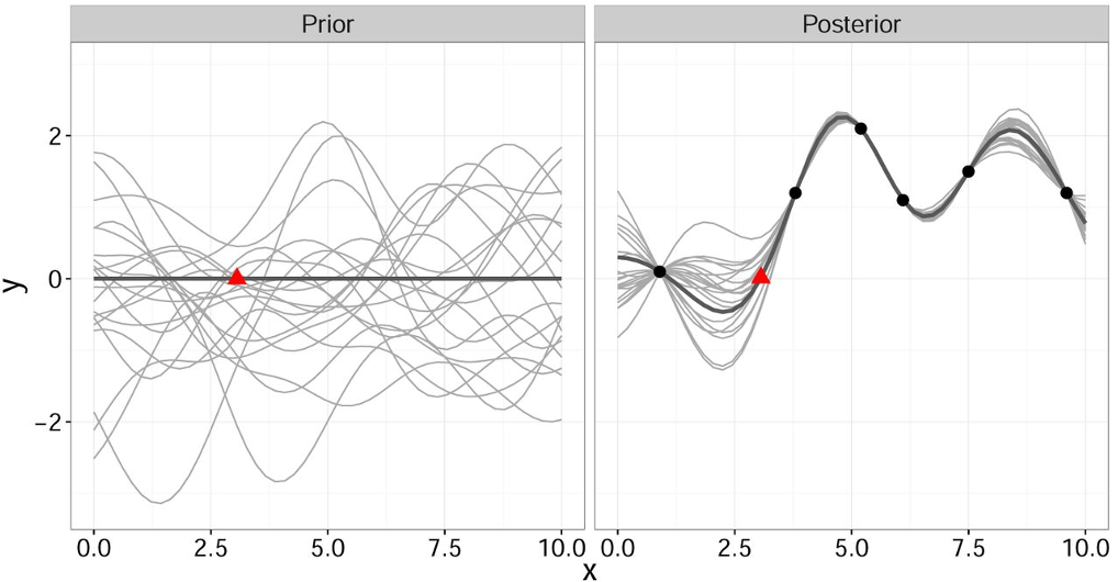
It is important to note that this gives a joint prior distribution of functions (Fig. 1 left, grey curves).
By restricting this distribution to contain only those functions (Fig. 1 right, grey curves) that agree with the observed data points [math]\displaystyle{ \mathbf{x} }[/math] (Fig. 1 right, solid black) we obtain the posterior distribution for [math]\displaystyle{ \hat{y} }[/math] which has the form
$$ p(\hat{y} | \mathbf{x}^*, X, \mathbf{y}) \sim \mathcal{N}(\mu(\mathbf{x}^*,X,\mathbf{y}),\sigma(\mathbf{x}^*,X)) $$
