Fix your classifier: the marginal value of training the last weight layer: Difference between revisions
No edit summary |
|||
| (47 intermediate revisions by 21 users not shown) | |||
| Line 1: | Line 1: | ||
This is a summary of the paper titled: "Fix your classifier: the marginal value of training the last weight layer", authored by Elad Hoffer, Itay Hubara, and Daniel Soudry. Available online at URL https://arxiv.org/abs/1801.04540 | |||
The code for the proposed model is available at https://github.com/eladhoffer/fix_your_classifier. | |||
=Introduction= | =Introduction= | ||
Deep neural networks have become | Deep neural networks have become widely used for machine learning, achieving state-of-the-art results on many tasks. One of the most common tasks they are used for is classification. For example, convolutional neural networks (CNNs) are used to classify images to a semantic category. Typically, a learned affine transformation is placed at the end of such models, yielding a per-class prediction for each class. This classifier can have a vast number of parameters, which grows linearly with the number of possible classes. As the number of classes in the data set increases, more and more computational resources are consumed by this layer. | ||
a vast number of parameters, which grows linearly with the number of possible classes, | |||
=Brief Overview= | =Brief Overview= | ||
In order to alleviate the aforementioned problem, the authors propose that the final layer of the classifier be fixed ( | In order to alleviate the aforementioned problem, the authors propose that the final layer of the classifier be fixed (up to a global scale constant). They argue that with little or no loss of accuracy for most classification tasks, the method provides significant memory and computational benefits. In addition, they show that by initializing the classifier with a Hadamard matrix the inference could be made faster as well. | ||
=Previous Work= | =Previous Work= | ||
Training | Training neural networks (NNs) and using them for inference requires large amounts of memory and computational resources; thus, extensive research has focused on reducing the size of these networks, including: | ||
* Weight sharing and specification (Han et al., 2015) | * Weight sharing and specification (Han et al., 2015). Weight sharing has to do with the filters used in the convolution layers. Normally, we would train different filters for each depth dimension. For example, in a particular convolution step, if our input was XxYx3, we would have 3 different filters applied to each 2D slice. Weight sharing forces the network to use identical filters for each of these layers. That is, the trained-for AxB convolution will have the same values, and the “stamp” will be identical; no matter which of the 3 dimensions is dealt with. | ||
* Mixed precision to reduce the size of the neural networks by half (Micikevicius et al., 2017) | * Mixed precision to reduce the size of the neural networks by half (Micikevicius et al., 2017) | ||
| Line 18: | Line 21: | ||
* Low-rank approximations to speed up CNN (Tai et al., 2015) | * Low-rank approximations to speed up CNN (Tai et al., 2015) | ||
* Quantization of weights, activations and gradients to further reduce computation during training (Hubara et al., 2016b; Li et al., 2016 and Zhou et al., 2016) | * Quantization of weights, activations, and gradients to further reduce computation during training (Hubara et al., 2016b; Li et al., 2016 and Zhou et al., 2016). Although aggressive quantization benefits from smaller model size, the extreme compression rate comes with a loss of accuracy. | ||
Some of the past works have also put forward the fact that predefined (Park & Sandberg, 1991) and random (Huang et al., 2006) projections can be used together with a learned affine transformation to achieve competitive results on many of the classification tasks. However, the authors' proposal in the current paper suggests the reverse proposal - common NN models can learn useful representations even without modifying the final output layer, which often holds a large number of parameters that grows linearly with number of classes. | |||
The use of a fixed transform can, in many cases, allow a huge decrease in model parameters, and | |||
a possible computational benefit. Authors suggest that existing models can, with no other modification, | |||
devoid their classifier weights, which can help the deployment of those models in devices with low | |||
computation ability and smaller memory capacity. | |||
=Background= | =Background= | ||
A CNN is comprised of one or more convolutional layers (often with a subsampling step) and then followed by one or more fully connected layers as in a standard multilayer neural network. The architecture of a CNN is designed to take advantage of the 2D structure of an input image (or other 2D input such as a speech signal). This is achieved with local connections and tied weights followed by some form of pooling which results in translation invariant features. Another benefit of CNNs is that they are easier to train and have many fewer parameters than fully connected networks with the same number of hidden units. | |||
= | A CNN consists of a number of convolutional and subsampling layers optionally followed by fully connected layers. The input to a convolutional layer is a <math>m \times m \times r</math> image where <math>m</math> is the height and width of the image and <math>r</math> is the number of channels, e.g. an RGB image has <math>r=3</math>. The convolutional layer can have a specifiable number of <math>k</math> filters (or kernels) of size <math>n \times n \times q</math> where <math>n</math> is the height and width of the kernel and is smaller than the dimension of the image, and <math>q</math> can either be the same or smaller that the number of channels in the previous layer. Each kernel is convolved with the image to produce <math>k</math> feature maps of size <math>m−n+1</math>. Each map is then subsampled typically with mean or max pooling over <math>p \times p</math> contiguous regions where <math>p</math> ranges between 2 for small images (e.g. MNIST) and is usually not more than 5 for larger inputs. Either before or after the subsampling layer an additive bias and sigmoidal nonlinearity is applied to each feature map. | ||
CNNs are commonly used to solve a variety of spatial and temporal tasks. Earlier architectures of CNNs (LeCun et al., 1998; Krizhevsky et al., 2012) used a set of fully-connected layers at later stages of the network, presumably to allow classification based on global features of an image. | |||
== Shortcomings of the Final Classification Layer == | |||
Zeiler & Fergus, 2014 showed that despite the enormous number of trainable parameters fully connected layers add to the model, they have a rather marginal impact on the performance. Furthermore, it has been shown that these layers could be easily compressed and reduced after a model is trained by simple means such as matrix decomposition and sparsification (Han et al., 2015). Modern NNs are characterized with the removal of most fully connected layers (Lin et al., 2013; Szegedy et al., 2015; He et al., 2016). This was shown to lead to better generalization and overall accuracy, together with a huge decrease in the number of trainable parameters. Additionally, numerous works showed that CNNs can be trained in a metric learning regime (Bromley et al., 1994; Schroff et al., 2015; Hoffer & Ailon, 2015), where no explicit classification layer is used and the objective regarded only distance measures between intermediate representations. Hardt & Ma (2017) suggested an all-convolutional network variant, where they kept the original initialization of the classification layer fixed and found no negative impact on performance on the CIFAR-10 dataset. | |||
=Proposed Method= | =Proposed Method= | ||
The aforementioned works provide evidence that fully-connected layers are in fact redundant and play a small role in learning and generalization. In this work, the authors have suggested that parameters used for the final classification transform are completely redundant, and can be replaced with a predetermined linear transform. This holds for even in large-scale models and classification tasks, such as recent architectures trained on the ImageNet benchmark (Deng et al., 2009). | The aforementioned works provide evidence that fully-connected layers are in fact redundant and play a small role in learning and generalization. In this work, the authors have suggested that the parameters used for the final classification transform are completely redundant, and can be replaced with a predetermined linear transform. This holds for even in large-scale models and classification tasks, such as recent architectures trained on the ImageNet benchmark (Deng et al., 2009). | ||
Such a use of fixed transform allows a huge decrease in model parameters and a possible computational benefit. Authors alos suggest that existing models can, with no other modifications devoid their classifier weights, which can help the deployment of those models in devices with low computational ability and smaller memory capacity. Hence as we keep the classifier fixed, less parameters need to be updated, reducing the communication cost of models deployed in a distributed systems. | |||
==Using a Fixed Classifier== | |||
In common NN models, this representation is followed by an additional affine transformation, <math>y = W^T x + b</math> ,where <math>W</math> and <math>b</math> are also trained by back-propagation. | Suppose the final representation obtained by the network (the last hidden layer) is represented as <math>x = F(z;\theta)</math> where <math>F</math> is assumed to be a deep neural network with input <math>z</math> and parameters <math>θ</math>, e.g., a convolutional network, trained by backpropagation. In common NN models, this representation is followed by an additional affine transformation, <math>y = W^T x + b</math>, where <math>W</math> and <math>b</math> are also trained by back-propagation. | ||
For input <math>x</math> of <math>N</math> | For input <math>x</math> of length <math>N</math>, and <math>C</math> different possible outputs, <math>W</math> is required to be a matrix of <math>N × C</math>. | ||
C</math>. | |||
Training is done using cross-entropy loss, by feeding the network outputs through a softmax activation | |||
v_i = \frac{e^{y_i}}{\sum_{j}^{C}{e^{y_j}}}, i | |||
\begin{align} | |||
v_i = \frac{e^{y_i}}{\sum_{j}^{C}{e^{y_j}}}, \qquad i \in {1, . . . , C} | |||
\end{align} | |||
and reducing the expected negative log likelihood with respect to ground-truth target <math> t | and reducing the expected negative log likelihood with respect to ground-truth target class <math> t </math>, by minimizing the loss function: | ||
by minimizing the loss function: | |||
\begin{align} | |||
L(x, t) = − log {v_t} = −{w_t}·{x} − b_t + log ({\sum_{j}^{C}e^{w_j . x + b_j}}) | L(x, t) = −\text{log}\ {v_t} = −{w_t}·{x} − b_t + \text{log} ({\sum_{j}^{C}e^{w_j . x + b_j}}) | ||
\end{align} | |||
where <math>w_i</math> is the <math>i</math>-th column of <math>W</math>. | where <math>w_i</math> is the <math>i</math>-th column of <math>W</math>. | ||
==Choosing the | ==Choosing the Projection Matrix== | ||
To evaluate the conjecture regarding the importance of the final classification transformation, the trainable parameter matrix <math>W</math> is replaced with a fixed orthonormal projection <math> Q ∈ R^{N×C} </math>, such that <math> ∀ i ≠ j : q_i · q_j = 0 </math> and <math> || q_i ||_{2} = 1 </math>, where <math>q_i</math> is the <math>i</math>th column of <math>Q</math>. This is ensured by a simple random sampling and singular-value decomposition | To evaluate the conjecture regarding the importance of the final classification transformation, the trainable parameter matrix <math>W</math> is replaced with a fixed orthonormal projection <math> Q ∈ R^{N×C} </math>, such that <math> ∀ i ≠ j : q_i · q_j = 0 </math> and <math> || q_i ||_{2} = 1 </math>, where <math>q_i</math> is the <math>i</math>th column of <math>Q</math>. This is ensured by a simple random sampling and singular-value decomposition | ||
| Line 68: | Line 80: | ||
</math></center> | </math></center> | ||
This allows faster training and convergence, as the network does not need to account for changes in the scale of its weights. However, it has now an issue that <math>q_i · \hat{x} </math> is bounded between −1 and 1. This causes convergence issues, as the softmax function is scale sensitive, and the network is affected by the inability to re-scale its input. This issue is amended with a fixed scale <math>T</math> applied to softmax inputs <math>f(y) = softmax(\frac{1}{T}y)</math>, also known as the ''softmax temperature''. However, this introduces an additional hyper-parameter which may differ between networks and datasets. So, the authors propose to introduce a single scalar parameter <math>\alpha</math> to learn the softmax scale, effectively functioning as an inverse of the softmax temperature <math>\frac{1}{T}</math>. The additional vector of bias parameters <math>b ∈ R^{C}</math> is kept the same and the model is trained using the traditional negative-log-likelihood criterion. Explicitly, the classifier output is now: | This allows faster training and convergence, as the network does not need to account for changes in the scale of its weights. However, it has now an issue that <math>q_i · \hat{x} </math> is bounded between −1 and 1. This causes convergence issues, as the softmax function is scale sensitive, and the network is affected by the inability to re-scale its input. This issue is amended with a fixed scale <math>T</math> applied to softmax inputs <math>f(y) = softmax(\frac{1}{T}y)</math>, also known as the ''softmax temperature''. However, this introduces an additional hyper-parameter which may differ between networks and datasets. So, the authors propose to introduce a single scalar parameter <math>\alpha</math> to learn the softmax scale, effectively functioning as an inverse of the softmax temperature <math>\frac{1}{T}</math>. The normalized weights and an additional scale coefficient are also used, specially using a single scale for all entries in the weight matrix. The additional vector of bias parameters <math>b ∈ \mathbb{R}^{C}</math> is kept the same and the model is trained using the traditional negative-log-likelihood criterion. Explicitly, the classifier output is now: | ||
<center> | <center> | ||
| Line 78: | Line 90: | ||
<center><math> | <center><math> | ||
L(x, t) = -\alpha q_t · \frac{x}{||x||_{2}} + b_t + log (\sum_{i=1}^{C} exp((\alpha q_i · \frac{x}{||x||_{2}} + b_i))) | L(x, t) = -\alpha q_t · \frac{x}{||x||_{2}} + b_t + \text{log} (\sum_{i=1}^{C} \text{exp}((\alpha q_i · \frac{x}{||x||_{2}} + b_i))) | ||
</math></center> | </math></center> | ||
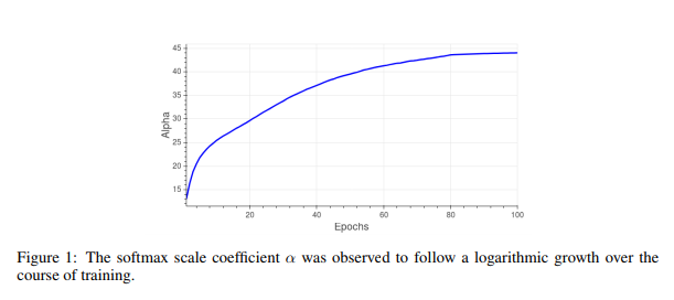
where <math>x</math> is the final representation obtained by the network for a specific sample, and <math> t ∈ </math> { <math> {1, . . . , C} </math> } is the ground-truth label for that sample. The behaviour of the parameter <math> \alpha </math> over time, which is logarithmic in nature, is shown in | where <math>x</math> is the final representation obtained by the network for a specific sample, and <math> t ∈ </math> { <math> {1, . . . , C} </math> } is the ground-truth label for that sample. The behaviour of the parameter <math> \alpha </math> over time, which is logarithmic in nature and has the same behavior exhibited by the norm of a learned classifier, is shown in | ||
[[Media: figure1_log_behave.png| Figure 1]]. | [[Media: figure1_log_behave.png| Figure 1]]. | ||
<center>[[File:figure1_log_behave.png]]</center> | <center>[[File:figure1_log_behave.png]]</center> | ||
==Using a | When <math> -1 \le q_i · \hat{x} \le 1 </math>, a possible cosine angle loss is | ||
<center>[[File:caloss.png]]</center> | |||
But its final validation accuracy has a slight decrease, compared to original models. | |||
==Using a Hadamard Matrix== | |||
To recall, Hadamard matrix (Hedayat et al., 1978) <math> H </math> is an <math> n × n </math> matrix, where all of its entries are either +1 or −1. | |||
Example: | |||
<math>\displaystyle H_{4}={\begin{bmatrix}1&1&1&1\\1&-1&1&-1\\1&1&-1&-1\\1&-1&-1&1\end{bmatrix}}</math> | |||
Furthermore, <math> H </math> is orthogonal, such that <math> HH^{T} = nI_n </math> where <math>I_n</math> is the identity matrix. Instead of using the entire Hadamard matrix <math>H</math>, a truncated version, <math> \hat{H} ∈ </math> {<math> {-1, 1}</math>}<math>^{C \times N}</math> where all <math>C</math> rows are orthogonal as the final classification layer is such that: | |||
Furthermore, <math> H </math> is orthogonal, such that <math> HH^{T} = nI_n </math> where <math>I_n</math> is the identity matrix. Instead of using the entire | |||
<center><math> | <center><math> | ||
| Line 107: | Line 129: | ||
==CIFAR-10/100== | ==CIFAR-10/100== | ||
===About the | ===About the Dataset=== | ||
CIFAR-10 is an image classification benchmark dataset containing 50,000 training images and 10,000 test images. The images are in color and contain 32×32 pixels. There are 10 possible classes of various animals and vehicles. CIFAR-100 holds the same number of images of same size, but contains 100 different classes. | CIFAR-10 is an image classification benchmark dataset containing 50,000 training images and 10,000 test images. The images are in color and contain 32×32 pixels. There are 10 possible classes of various animals and vehicles. CIFAR-100 holds the same number of images of the same size, but contains 100 different classes. | ||
===Training Details=== | ===Training Details=== | ||
| Line 117: | Line 139: | ||
<center>[[File: figure1_resnet_cifar10.png]]</center> | <center>[[File: figure1_resnet_cifar10.png]]</center> | ||
These results demonstrate that although the training error is considerably lower for the network with learned classifier, both models achieve the same classification accuracy on the validation set. The authors conjecture is that with the new fixed parameterization, the network can no longer increase the | These results demonstrate that although the training error is considerably lower for the network with learned classifier, both models achieve the same classification accuracy on the validation set. The authors' conjecture is that with the new fixed parameterization, the network can no longer increase the norm of a given sample’s representation - thus learning its label requires more effort. As this may happen for specific seen samples - it affects only training error. | ||
norm of a given sample’s representation - thus learning its label requires more effort. As this may happen for specific seen samples - it affects only training error. | |||
The authors also compared using a fixed scale variable <math>\alpha </math> at different values vs. the learned parameter. Results for <math> \alpha = </math> {0.1, 1, 10} are depicted in [[Media: figure3_alpha_resnet_cifar.png| Figure 3]] for both training and validation error and as can be seen, similar validation accuracy can be obtained using a fixed scale value (in this case <math>\alpha </math>= 1 or 10 will suffice) at the expense of another hyper-parameter to seek. In all the further experiments the scaling parameter <math> \alpha </math> was regularized with the same weight decay coefficient used on original classifier. | The authors also compared using a fixed scale variable <math>\alpha </math> at different values vs. the learned parameter. Results for <math> \alpha = </math> {0.1, 1, 10} are depicted in [[Media: figure3_alpha_resnet_cifar.png| Figure 3]] for both training and validation error and as can be seen, similar validation accuracy can be obtained using a fixed scale value (in this case <math>\alpha </math>= 1 or 10 will suffice) at the expense of another hyper-parameter to seek. In all the further experiments the scaling parameter <math> \alpha </math> was regularized with the same weight decay coefficient used on original classifier. Although learning the scale is not necessary, but it will help convergence during training. | ||
<center>[[File: figure3_alpha_resnet_cifar.png]]</center> | <center>[[File: figure3_alpha_resnet_cifar.png]]</center> | ||
The authors then train the model on CIFAR-100 dataset. They used the DenseNet-BC model from Huang et al. (2017) with depth of 100 layers and k = 12. The higher number of classes caused the number of parameters to grow and encompassed about 4% of the whole model. However, validation accuracy for the fixed-classifier model remained equally good as the original model, and the same training curve was observed as earlier. | The authors then train the model on CIFAR-100 dataset. They used the DenseNet-BC model from Huang et al. (2017) with a depth of 100 layers and k = 12. The higher number of classes caused the number of parameters to grow and encompassed about 4% of the whole model. However, validation accuracy for the fixed-classifier model remained equally good as the original model, and the same training curve was observed as earlier. | ||
==IMAGENET== | ==IMAGENET== | ||
===About the | ===About the Dataset=== | ||
The Imagenet dataset introduced by Deng et al. (2009) spans over 1000 visual classes, and over 1.2 million samples. This is supposedly a more challenging dataset to work on as compared to CIFAR-10/100. | The Imagenet dataset introduced by Deng et al. (2009) spans over 1000 visual classes, and over 1.2 million samples. This is supposedly a more challenging dataset to work on as compared to CIFAR-10/100. | ||
| Line 136: | Line 157: | ||
The authors evaluated their fixed classifier method on Imagenet using Resnet50 by He et al. (2016) and Densenet169 model (Huang et al., 2017) as described in the original work. Using a fixed classifier removed approximately 2-million parameters were from the model, accounting for about 8% and 12 % of the model parameters respectively. The experiments revealed similar trends as observed on CIFAR-10. | The authors evaluated their fixed classifier method on Imagenet using Resnet50 by He et al. (2016) and Densenet169 model (Huang et al., 2017) as described in the original work. Using a fixed classifier removed approximately 2-million parameters were from the model, accounting for about 8% and 12 % of the model parameters respectively. The experiments revealed similar trends as observed on CIFAR-10. | ||
For a more stricter evaluation, the authors also trained a Shufflenet architecture (Zhang et al., 2017b), which was designed to be used in low memory and limited computing platforms and has parameters making up the majority of the model. They were able to reduce the parameters to 0.86 million as compared to 0.96 million parameters in the final layer of the original model. Again, the proposed modification in the original model gave similar convergence results on validation accuracy. | For a more stricter evaluation, the authors also trained a Shufflenet architecture (Zhang et al., 2017b), which was designed to be used in low memory and limited computing platforms and has parameters making up the majority of the model. They were able to reduce the parameters to 0.86 million as compared to 0.96 million parameters in the final layer of the original model. Again, the proposed modification in the original model gave similar convergence results on validation accuracy. Interestingly, this method allowed Imagenet training in an under-specified regime, where there are | ||
more training samples than the number of parameters. This is an unconventional regime for modern deep networks, which are usually over-specified to have many more parameters than training samples (Zhang et al., 2017a). | |||
The overall results of the fixed-classifier are summarized in [[Media: table1_fixed_results.png | Table 1]]. | The overall results of the fixed-classifier are summarized in [[Media: table1_fixed_results.png | Table 1]]. | ||
| Line 144: | Line 166: | ||
==Language Modelling== | ==Language Modelling== | ||
Recent works have empirically found that using the same weights for both word embedding and classifier can yield equal or better results than using a separate pair of weights. So the authors experimented with fix-classifiers on language modeling as it also requires classification of all possible tokens available in the task vocabulary. They trained a recurrent model with 2-layers of LSTM (Hochreiter & Schmidhuber, 1997) and embedding + hidden size of 512 on the WikiText2 dataset (Merity et al., 2016), using same settings as in Merity et al. (2017). WikiText2 dataset contains about 33K different words, so the number of parameters expected in the embedding and classifier layer was about 34-million. This number is about 89% of the total number of parameters used for the whole model which is 38-million. However, using a random orthogonal transform yielded poor results compared to learned embedding. This was suspected to be due to semantic relationships captured in the embedding layer of language models, which is not the case in image classification task. The intuition was further confirmed by the much better results when pre-trained embeddings using word2vec algorithm by Mikolov et al. (2013) or PMI factorization as suggested by Levy & Goldberg (2014), were used. The final result used 89% fewer parameters than a fully learned model, with only marginally worse perplexity. The authors posit that this implies a required structure in word embedding that originates from the semantic relatedness between words, and unbalanced classes. They further suggest that with more efficient ways to train word embeddings, it may be possible to mitigate the issues arising from this structure and class imbalance. | |||
<center>[[File: language.png]]</center> | |||
=Discussion= | =Discussion= | ||
==Implications and | ==Implications and Use Cases== | ||
With the increasing number of classes in the benchmark datasets, computational demands for the final classifier will increase as well. In order to understand the problem better, the authors observe the work by Sun et al. (2017), which introduced JFT-300M - an internal Google dataset with over 18K different classes. Using a Resnet50 (He et al., 2016), with a 2048 sized representation led to a model with over 36M parameters meaning that over 60% of the model parameters resided in the final classification layer. Sun et al. (2017) also describe the difficulty in distributing so many parameters over the training servers involving a non-trivial overhead during synchronization of the model for update. The authors claim that the fixed-classifier would help considerably in this kind of scenario - where using a fixed classifier removes the need to do any gradient synchronization for the final layer. Furthermore, introduction of Hadamard matrix removes the need to save the transformation altogether, thereby, making it more efficient and allowing considerable memory and computational savings. | With the increasing number of classes in the benchmark datasets, computational demands for the final classifier will increase as well. In order to understand the problem better, the authors observe the work by Sun et al. (2017), which introduced JFT-300M - an internal Google dataset with over 18K different classes. Using a Resnet50 (He et al., 2016), with a 2048 sized representation led to a model with over 36M parameters meaning that over 60% of the model parameters resided in the final classification layer. Sun et al. (2017) also describe the difficulty in distributing so many parameters over the training servers involving a non-trivial overhead during synchronization of the model for update. The authors claim that the fixed-classifier would help considerably in this kind of scenario - where using a fixed classifier removes the need to do any gradient synchronization for the final layer. Furthermore, introduction of Hadamard matrix removes the need to save the transformation altogether, thereby, making it more efficient and allowing considerable memory and computational savings. | ||
| Line 155: | Line 178: | ||
==Possible Caveats== | ==Possible Caveats== | ||
The good performance of fixed-classifiers relies on the ability of the preceding layers to learn separable representations. This could be affected | The good performance of fixed-classifiers relies on the ability of the preceding layers to learn separable representations. This could be affected when the ratio between learned features and number of classes is small – that is, when <math> C > N</math>. However, they tested their method in such cases and their model performed well and provided good results. | ||
Some experiments were conducted by the authors with such cases, for example Imagenet classification (C = 1000) using mobilenet-0.5 with N = 512 or using ResNet with N = 256. In both scenarios, this method converged similarly to a fully learned classifier reaching the same final validation accuracy. Although, there is no presentation of this information within the paper itself, if true, it may strengthen the finding that even in cases in which C > N, fixed classifier can provide equally good results. | |||
Another factor that can affect the performance of their model using a fixed classifier is when the classes are highly correlated. In that case, the fixed classifier actually cannot support correlated classes and thus, the network could have some difficulty to learn. For a language model, word classes tend to have highly correlated instances, which also lead to difficult learning process. | |||
Also, this proposed approach will only eliminate the computation of the classifier weights, so when the classes are fewer, the computation saving effect will not be readily apparent. | |||
==Future Work== | ==Future Work== | ||
The use of fixed classifiers might be further simplified in Binarized Neural Networks (Hubara et al., 2016a), where the activations and weights are restricted to ±1 during propagations. In that case the norm of the last hidden layer would be constant for all samples (equal to the square root of the hidden layer width). The constant could then be absorbed into the scale constant <math>\alpha</math>, and there is no need in a per-sample normalization. | The use of fixed classifiers might be further simplified in Binarized Neural Networks (Hubara et al., 2016a), where the activations and weights are restricted to ±1 during propagations. In that case, the norm of the last hidden layer would be constant for all samples (equal to the square root of the hidden layer width). The constant could then be absorbed into the scale constant <math>\alpha</math>, and there is no need in a per-sample normalization. | ||
Additionally, more efficient ways to learn a word embedding should also be explored where similar redundancy in classifier weights may suggest simpler forms of token representations - such as low-rank or sparse versions. | Additionally, more efficient ways to learn a word embedding should also be explored where similar redundancy in classifier weights may suggest simpler forms of token representations - such as low-rank or sparse versions. | ||
| Line 170: | Line 199: | ||
In this work, the authors argue that the final classification layer in deep neural networks is redundant and suggest removing the parameters from the classification layer. The empirical results from experiments on the CIFAR and IMAGENET datasets suggest that such a change lead to little or almost no decline in the performance of the architecture. Furthermore, using a Hadmard matrix as classifier might lead to some computational benefits when properly implemented, and save memory otherwise spent on large amount of transformation coefficients. | In this work, the authors argue that the final classification layer in deep neural networks is redundant and suggest removing the parameters from the classification layer. The empirical results from experiments on the CIFAR and IMAGENET datasets suggest that such a change lead to little or almost no decline in the performance of the architecture. Furthermore, using a Hadmard matrix as classifier might lead to some computational benefits when properly implemented, and save memory otherwise spent on large amount of transformation coefficients. | ||
Another possible scope of research that could be pointed out for future could be to find new efficient methods to create pre-defined word embeddings, which require huge amount of parameters that can possibly be avoided when learning a new task. Therefore, more emphasis should be given to the representations learned by the non-linear parts of the neural networks - | Another possible scope of research that could be pointed out for future could be to find new efficient methods to create pre-defined word embeddings, which require huge amount of parameters that can possibly be avoided when learning a new task. Therefore, more emphasis should be given to the representations learned by the non-linear parts of the neural networks - up to the final classifier, as it seems highly redundant. | ||
=Critique= | =Critique= | ||
The paper proposes an interesting idea that has a potential use case when designing memory-efficient neural networks. The experiments shown in the paper are quite rigorous and provide support to the authors' claim. However, it would have been more helpful if the authors had described a bit more about efficient implementation of the Hadamard matrix and how to scale this method for larger datasets (cases with <math> C >N</math>). | The paper proposes an interesting idea that has a potential use case when designing memory-efficient neural networks. The experiments shown in the paper are quite rigorous and provide support to the authors' claim. However, it would have been more helpful if the authors had described a bit more about efficient implementation of the Hadamard matrix and how to scale this method for larger datasets (cases with <math> C >N</math>). | ||
Moreover, one of the main intuitions of the paper has introduced to be computational cost but it has left out to compare a fixed and learned classifier based on the computational cost and then investigate whether it worth the drop in performance or not considering the fact that not always the output can be degraded because of need for speed! At least a discussion on this issue is expected. | |||
On the other hand, the computational cost and performance change after fixation of classifier could be related to dataset and the nature and complexity of it. Mostly, having 1000 classes makes the classification more crucial than 2 classes. An evaluation of this topic is also needed. | |||
Another interesting experiment to do would be to look this technique interacts with distillation when used in the teacher or student network or both. For instance, Does fixing the features make it more difficult to place dog than on boat when classifying a cat? Do networks with fixed classifier weights make worse teachers for distillation? | |||
=References= | =References= | ||
Madhu S Advani and Andrew M Saxe. High-dimensional dynamics of generalization error in neural networks. arXiv preprint arXiv:1710.03667, 2017. | Madhu S Advani and Andrew M Saxe. High-dimensional dynamics of generalization error in neural networks. arXiv preprint arXiv:1710.03667, 2017. | ||
Latest revision as of 00:39, 17 December 2018
This is a summary of the paper titled: "Fix your classifier: the marginal value of training the last weight layer", authored by Elad Hoffer, Itay Hubara, and Daniel Soudry. Available online at URL https://arxiv.org/abs/1801.04540
The code for the proposed model is available at https://github.com/eladhoffer/fix_your_classifier.
Introduction
Deep neural networks have become widely used for machine learning, achieving state-of-the-art results on many tasks. One of the most common tasks they are used for is classification. For example, convolutional neural networks (CNNs) are used to classify images to a semantic category. Typically, a learned affine transformation is placed at the end of such models, yielding a per-class prediction for each class. This classifier can have a vast number of parameters, which grows linearly with the number of possible classes. As the number of classes in the data set increases, more and more computational resources are consumed by this layer.
Brief Overview
In order to alleviate the aforementioned problem, the authors propose that the final layer of the classifier be fixed (up to a global scale constant). They argue that with little or no loss of accuracy for most classification tasks, the method provides significant memory and computational benefits. In addition, they show that by initializing the classifier with a Hadamard matrix the inference could be made faster as well.
Previous Work
Training neural networks (NNs) and using them for inference requires large amounts of memory and computational resources; thus, extensive research has focused on reducing the size of these networks, including:
- Weight sharing and specification (Han et al., 2015). Weight sharing has to do with the filters used in the convolution layers. Normally, we would train different filters for each depth dimension. For example, in a particular convolution step, if our input was XxYx3, we would have 3 different filters applied to each 2D slice. Weight sharing forces the network to use identical filters for each of these layers. That is, the trained-for AxB convolution will have the same values, and the “stamp” will be identical; no matter which of the 3 dimensions is dealt with.
- Mixed precision to reduce the size of the neural networks by half (Micikevicius et al., 2017)
- Low-rank approximations to speed up CNN (Tai et al., 2015)
- Quantization of weights, activations, and gradients to further reduce computation during training (Hubara et al., 2016b; Li et al., 2016 and Zhou et al., 2016). Although aggressive quantization benefits from smaller model size, the extreme compression rate comes with a loss of accuracy.
Some of the past works have also put forward the fact that predefined (Park & Sandberg, 1991) and random (Huang et al., 2006) projections can be used together with a learned affine transformation to achieve competitive results on many of the classification tasks. However, the authors' proposal in the current paper suggests the reverse proposal - common NN models can learn useful representations even without modifying the final output layer, which often holds a large number of parameters that grows linearly with number of classes.
The use of a fixed transform can, in many cases, allow a huge decrease in model parameters, and a possible computational benefit. Authors suggest that existing models can, with no other modification, devoid their classifier weights, which can help the deployment of those models in devices with low computation ability and smaller memory capacity.
Background
A CNN is comprised of one or more convolutional layers (often with a subsampling step) and then followed by one or more fully connected layers as in a standard multilayer neural network. The architecture of a CNN is designed to take advantage of the 2D structure of an input image (or other 2D input such as a speech signal). This is achieved with local connections and tied weights followed by some form of pooling which results in translation invariant features. Another benefit of CNNs is that they are easier to train and have many fewer parameters than fully connected networks with the same number of hidden units.
A CNN consists of a number of convolutional and subsampling layers optionally followed by fully connected layers. The input to a convolutional layer is a [math]\displaystyle{ m \times m \times r }[/math] image where [math]\displaystyle{ m }[/math] is the height and width of the image and [math]\displaystyle{ r }[/math] is the number of channels, e.g. an RGB image has [math]\displaystyle{ r=3 }[/math]. The convolutional layer can have a specifiable number of [math]\displaystyle{ k }[/math] filters (or kernels) of size [math]\displaystyle{ n \times n \times q }[/math] where [math]\displaystyle{ n }[/math] is the height and width of the kernel and is smaller than the dimension of the image, and [math]\displaystyle{ q }[/math] can either be the same or smaller that the number of channels in the previous layer. Each kernel is convolved with the image to produce [math]\displaystyle{ k }[/math] feature maps of size [math]\displaystyle{ m−n+1 }[/math]. Each map is then subsampled typically with mean or max pooling over [math]\displaystyle{ p \times p }[/math] contiguous regions where [math]\displaystyle{ p }[/math] ranges between 2 for small images (e.g. MNIST) and is usually not more than 5 for larger inputs. Either before or after the subsampling layer an additive bias and sigmoidal nonlinearity is applied to each feature map.
CNNs are commonly used to solve a variety of spatial and temporal tasks. Earlier architectures of CNNs (LeCun et al., 1998; Krizhevsky et al., 2012) used a set of fully-connected layers at later stages of the network, presumably to allow classification based on global features of an image.
Shortcomings of the Final Classification Layer
Zeiler & Fergus, 2014 showed that despite the enormous number of trainable parameters fully connected layers add to the model, they have a rather marginal impact on the performance. Furthermore, it has been shown that these layers could be easily compressed and reduced after a model is trained by simple means such as matrix decomposition and sparsification (Han et al., 2015). Modern NNs are characterized with the removal of most fully connected layers (Lin et al., 2013; Szegedy et al., 2015; He et al., 2016). This was shown to lead to better generalization and overall accuracy, together with a huge decrease in the number of trainable parameters. Additionally, numerous works showed that CNNs can be trained in a metric learning regime (Bromley et al., 1994; Schroff et al., 2015; Hoffer & Ailon, 2015), where no explicit classification layer is used and the objective regarded only distance measures between intermediate representations. Hardt & Ma (2017) suggested an all-convolutional network variant, where they kept the original initialization of the classification layer fixed and found no negative impact on performance on the CIFAR-10 dataset.
Proposed Method
The aforementioned works provide evidence that fully-connected layers are in fact redundant and play a small role in learning and generalization. In this work, the authors have suggested that the parameters used for the final classification transform are completely redundant, and can be replaced with a predetermined linear transform. This holds for even in large-scale models and classification tasks, such as recent architectures trained on the ImageNet benchmark (Deng et al., 2009).
Such a use of fixed transform allows a huge decrease in model parameters and a possible computational benefit. Authors alos suggest that existing models can, with no other modifications devoid their classifier weights, which can help the deployment of those models in devices with low computational ability and smaller memory capacity. Hence as we keep the classifier fixed, less parameters need to be updated, reducing the communication cost of models deployed in a distributed systems.
Using a Fixed Classifier
Suppose the final representation obtained by the network (the last hidden layer) is represented as [math]\displaystyle{ x = F(z;\theta) }[/math] where [math]\displaystyle{ F }[/math] is assumed to be a deep neural network with input [math]\displaystyle{ z }[/math] and parameters [math]\displaystyle{ θ }[/math], e.g., a convolutional network, trained by backpropagation. In common NN models, this representation is followed by an additional affine transformation, [math]\displaystyle{ y = W^T x + b }[/math], where [math]\displaystyle{ W }[/math] and [math]\displaystyle{ b }[/math] are also trained by back-propagation.
For input [math]\displaystyle{ x }[/math] of length [math]\displaystyle{ N }[/math], and [math]\displaystyle{ C }[/math] different possible outputs, [math]\displaystyle{ W }[/math] is required to be a matrix of [math]\displaystyle{ N × C }[/math].
Training is done using cross-entropy loss, by feeding the network outputs through a softmax activation
\begin{align} v_i = \frac{e^{y_i}}{\sum_{j}^{C}{e^{y_j}}}, \qquad i \in {1, . . . , C} \end{align}
and reducing the expected negative log likelihood with respect to ground-truth target class [math]\displaystyle{ t }[/math], by minimizing the loss function:
\begin{align} L(x, t) = −\text{log}\ {v_t} = −{w_t}·{x} − b_t + \text{log} ({\sum_{j}^{C}e^{w_j . x + b_j}}) \end{align}
where [math]\displaystyle{ w_i }[/math] is the [math]\displaystyle{ i }[/math]-th column of [math]\displaystyle{ W }[/math].
Choosing the Projection Matrix
To evaluate the conjecture regarding the importance of the final classification transformation, the trainable parameter matrix [math]\displaystyle{ W }[/math] is replaced with a fixed orthonormal projection [math]\displaystyle{ Q ∈ R^{N×C} }[/math], such that [math]\displaystyle{ ∀ i ≠ j : q_i · q_j = 0 }[/math] and [math]\displaystyle{ || q_i ||_{2} = 1 }[/math], where [math]\displaystyle{ q_i }[/math] is the [math]\displaystyle{ i }[/math]th column of [math]\displaystyle{ Q }[/math]. This is ensured by a simple random sampling and singular-value decomposition
As the rows of classifier weight matrix are fixed with an equally valued [math]\displaystyle{ L_{2} }[/math] norm, we find it beneficial to also restrict the representation of [math]\displaystyle{ x }[/math] by normalizing it to reside on the [math]\displaystyle{ n }[/math]-dimensional sphere:
This allows faster training and convergence, as the network does not need to account for changes in the scale of its weights. However, it has now an issue that [math]\displaystyle{ q_i · \hat{x} }[/math] is bounded between −1 and 1. This causes convergence issues, as the softmax function is scale sensitive, and the network is affected by the inability to re-scale its input. This issue is amended with a fixed scale [math]\displaystyle{ T }[/math] applied to softmax inputs [math]\displaystyle{ f(y) = softmax(\frac{1}{T}y) }[/math], also known as the softmax temperature. However, this introduces an additional hyper-parameter which may differ between networks and datasets. So, the authors propose to introduce a single scalar parameter [math]\displaystyle{ \alpha }[/math] to learn the softmax scale, effectively functioning as an inverse of the softmax temperature [math]\displaystyle{ \frac{1}{T} }[/math]. The normalized weights and an additional scale coefficient are also used, specially using a single scale for all entries in the weight matrix. The additional vector of bias parameters [math]\displaystyle{ b ∈ \mathbb{R}^{C} }[/math] is kept the same and the model is trained using the traditional negative-log-likelihood criterion. Explicitly, the classifier output is now:
[math]\displaystyle{ v_i=\frac{e^{\alpha q_i · \hat{x} + b_i}}{\sum_{j}^{C} e^{\alpha q_j · \hat{x} + b_j}}, i ∈ }[/math] { [math]\displaystyle{ {1,...,C} }[/math]}
and the loss to be minimized is:
where [math]\displaystyle{ x }[/math] is the final representation obtained by the network for a specific sample, and [math]\displaystyle{ t ∈ }[/math] { [math]\displaystyle{ {1, . . . , C} }[/math] } is the ground-truth label for that sample. The behaviour of the parameter [math]\displaystyle{ \alpha }[/math] over time, which is logarithmic in nature and has the same behavior exhibited by the norm of a learned classifier, is shown in Figure 1.

When [math]\displaystyle{ -1 \le q_i · \hat{x} \le 1 }[/math], a possible cosine angle loss is

But its final validation accuracy has a slight decrease, compared to original models.
Using a Hadamard Matrix
To recall, Hadamard matrix (Hedayat et al., 1978) [math]\displaystyle{ H }[/math] is an [math]\displaystyle{ n × n }[/math] matrix, where all of its entries are either +1 or −1. Example:
[math]\displaystyle{ \displaystyle H_{4}={\begin{bmatrix}1&1&1&1\\1&-1&1&-1\\1&1&-1&-1\\1&-1&-1&1\end{bmatrix}} }[/math]
Furthermore, [math]\displaystyle{ H }[/math] is orthogonal, such that [math]\displaystyle{ HH^{T} = nI_n }[/math] where [math]\displaystyle{ I_n }[/math] is the identity matrix. Instead of using the entire Hadamard matrix [math]\displaystyle{ H }[/math], a truncated version, [math]\displaystyle{ \hat{H} ∈ }[/math] {[math]\displaystyle{ {-1, 1} }[/math]}[math]\displaystyle{ ^{C \times N} }[/math] where all [math]\displaystyle{ C }[/math] rows are orthogonal as the final classification layer is such that:
This usage allows two main benefits:
- A deterministic, low-memory and easily generated matrix that can be used for classification.
- Removal of the need to perform a full matrix-matrix multiplication - as multiplying by a Hadamard matrix can be done by simple sign manipulation and addition.
Here, [math]\displaystyle{ n }[/math] must be a multiple of 4, but it can be easily truncated to fit normally defined networks. Also, as the classifier weights are fixed to need only 1-bit precision, it is now possible to focus our attention on the features preceding it.
Experimental Results
The authors have evaluated their proposed model on the following datasets:
CIFAR-10/100
About the Dataset
CIFAR-10 is an image classification benchmark dataset containing 50,000 training images and 10,000 test images. The images are in color and contain 32×32 pixels. There are 10 possible classes of various animals and vehicles. CIFAR-100 holds the same number of images of the same size, but contains 100 different classes.
Training Details
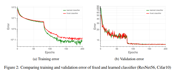
The authors trained a residual network ( He et al., 2016) on the CIFAR-10 dataset. The network depth was 56 and the same hyper-parameters as in the original work were used. A comparison of the two variants, i.e., the learned classifier and the proposed classifier with a fixed transformation is shown in Figure 2.

These results demonstrate that although the training error is considerably lower for the network with learned classifier, both models achieve the same classification accuracy on the validation set. The authors' conjecture is that with the new fixed parameterization, the network can no longer increase the norm of a given sample’s representation - thus learning its label requires more effort. As this may happen for specific seen samples - it affects only training error.
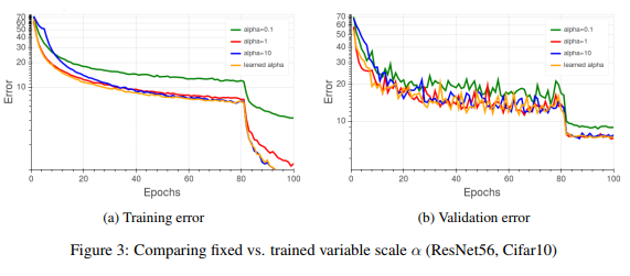
The authors also compared using a fixed scale variable [math]\displaystyle{ \alpha }[/math] at different values vs. the learned parameter. Results for [math]\displaystyle{ \alpha = }[/math] {0.1, 1, 10} are depicted in Figure 3 for both training and validation error and as can be seen, similar validation accuracy can be obtained using a fixed scale value (in this case [math]\displaystyle{ \alpha }[/math]= 1 or 10 will suffice) at the expense of another hyper-parameter to seek. In all the further experiments the scaling parameter [math]\displaystyle{ \alpha }[/math] was regularized with the same weight decay coefficient used on original classifier. Although learning the scale is not necessary, but it will help convergence during training.

The authors then train the model on CIFAR-100 dataset. They used the DenseNet-BC model from Huang et al. (2017) with a depth of 100 layers and k = 12. The higher number of classes caused the number of parameters to grow and encompassed about 4% of the whole model. However, validation accuracy for the fixed-classifier model remained equally good as the original model, and the same training curve was observed as earlier.
IMAGENET
About the Dataset
The Imagenet dataset introduced by Deng et al. (2009) spans over 1000 visual classes, and over 1.2 million samples. This is supposedly a more challenging dataset to work on as compared to CIFAR-10/100.
Experiment Details
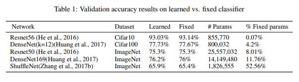
The authors evaluated their fixed classifier method on Imagenet using Resnet50 by He et al. (2016) and Densenet169 model (Huang et al., 2017) as described in the original work. Using a fixed classifier removed approximately 2-million parameters were from the model, accounting for about 8% and 12 % of the model parameters respectively. The experiments revealed similar trends as observed on CIFAR-10.
For a more stricter evaluation, the authors also trained a Shufflenet architecture (Zhang et al., 2017b), which was designed to be used in low memory and limited computing platforms and has parameters making up the majority of the model. They were able to reduce the parameters to 0.86 million as compared to 0.96 million parameters in the final layer of the original model. Again, the proposed modification in the original model gave similar convergence results on validation accuracy. Interestingly, this method allowed Imagenet training in an under-specified regime, where there are more training samples than the number of parameters. This is an unconventional regime for modern deep networks, which are usually over-specified to have many more parameters than training samples (Zhang et al., 2017a).
The overall results of the fixed-classifier are summarized in Table 1.

Language Modelling
Recent works have empirically found that using the same weights for both word embedding and classifier can yield equal or better results than using a separate pair of weights. So the authors experimented with fix-classifiers on language modeling as it also requires classification of all possible tokens available in the task vocabulary. They trained a recurrent model with 2-layers of LSTM (Hochreiter & Schmidhuber, 1997) and embedding + hidden size of 512 on the WikiText2 dataset (Merity et al., 2016), using same settings as in Merity et al. (2017). WikiText2 dataset contains about 33K different words, so the number of parameters expected in the embedding and classifier layer was about 34-million. This number is about 89% of the total number of parameters used for the whole model which is 38-million. However, using a random orthogonal transform yielded poor results compared to learned embedding. This was suspected to be due to semantic relationships captured in the embedding layer of language models, which is not the case in image classification task. The intuition was further confirmed by the much better results when pre-trained embeddings using word2vec algorithm by Mikolov et al. (2013) or PMI factorization as suggested by Levy & Goldberg (2014), were used. The final result used 89% fewer parameters than a fully learned model, with only marginally worse perplexity. The authors posit that this implies a required structure in word embedding that originates from the semantic relatedness between words, and unbalanced classes. They further suggest that with more efficient ways to train word embeddings, it may be possible to mitigate the issues arising from this structure and class imbalance.

Discussion
Implications and Use Cases
With the increasing number of classes in the benchmark datasets, computational demands for the final classifier will increase as well. In order to understand the problem better, the authors observe the work by Sun et al. (2017), which introduced JFT-300M - an internal Google dataset with over 18K different classes. Using a Resnet50 (He et al., 2016), with a 2048 sized representation led to a model with over 36M parameters meaning that over 60% of the model parameters resided in the final classification layer. Sun et al. (2017) also describe the difficulty in distributing so many parameters over the training servers involving a non-trivial overhead during synchronization of the model for update. The authors claim that the fixed-classifier would help considerably in this kind of scenario - where using a fixed classifier removes the need to do any gradient synchronization for the final layer. Furthermore, introduction of Hadamard matrix removes the need to save the transformation altogether, thereby, making it more efficient and allowing considerable memory and computational savings.
Possible Caveats
The good performance of fixed-classifiers relies on the ability of the preceding layers to learn separable representations. This could be affected when the ratio between learned features and number of classes is small – that is, when [math]\displaystyle{ C \gt N }[/math]. However, they tested their method in such cases and their model performed well and provided good results.
Some experiments were conducted by the authors with such cases, for example Imagenet classification (C = 1000) using mobilenet-0.5 with N = 512 or using ResNet with N = 256. In both scenarios, this method converged similarly to a fully learned classifier reaching the same final validation accuracy. Although, there is no presentation of this information within the paper itself, if true, it may strengthen the finding that even in cases in which C > N, fixed classifier can provide equally good results.
Another factor that can affect the performance of their model using a fixed classifier is when the classes are highly correlated. In that case, the fixed classifier actually cannot support correlated classes and thus, the network could have some difficulty to learn. For a language model, word classes tend to have highly correlated instances, which also lead to difficult learning process.
Also, this proposed approach will only eliminate the computation of the classifier weights, so when the classes are fewer, the computation saving effect will not be readily apparent.
Future Work
The use of fixed classifiers might be further simplified in Binarized Neural Networks (Hubara et al., 2016a), where the activations and weights are restricted to ±1 during propagations. In that case, the norm of the last hidden layer would be constant for all samples (equal to the square root of the hidden layer width). The constant could then be absorbed into the scale constant [math]\displaystyle{ \alpha }[/math], and there is no need in a per-sample normalization.
Additionally, more efficient ways to learn a word embedding should also be explored where similar redundancy in classifier weights may suggest simpler forms of token representations - such as low-rank or sparse versions.
A related paper was published that claims that fixing most of the parameters of the neural network achieves comparable results with learning all of them [A. Rosenfeld and J. K. Tsotsos]
Conclusion
In this work, the authors argue that the final classification layer in deep neural networks is redundant and suggest removing the parameters from the classification layer. The empirical results from experiments on the CIFAR and IMAGENET datasets suggest that such a change lead to little or almost no decline in the performance of the architecture. Furthermore, using a Hadmard matrix as classifier might lead to some computational benefits when properly implemented, and save memory otherwise spent on large amount of transformation coefficients.
Another possible scope of research that could be pointed out for future could be to find new efficient methods to create pre-defined word embeddings, which require huge amount of parameters that can possibly be avoided when learning a new task. Therefore, more emphasis should be given to the representations learned by the non-linear parts of the neural networks - up to the final classifier, as it seems highly redundant.
Critique
The paper proposes an interesting idea that has a potential use case when designing memory-efficient neural networks. The experiments shown in the paper are quite rigorous and provide support to the authors' claim. However, it would have been more helpful if the authors had described a bit more about efficient implementation of the Hadamard matrix and how to scale this method for larger datasets (cases with [math]\displaystyle{ C \gt N }[/math]).
Moreover, one of the main intuitions of the paper has introduced to be computational cost but it has left out to compare a fixed and learned classifier based on the computational cost and then investigate whether it worth the drop in performance or not considering the fact that not always the output can be degraded because of need for speed! At least a discussion on this issue is expected.
On the other hand, the computational cost and performance change after fixation of classifier could be related to dataset and the nature and complexity of it. Mostly, having 1000 classes makes the classification more crucial than 2 classes. An evaluation of this topic is also needed.
Another interesting experiment to do would be to look this technique interacts with distillation when used in the teacher or student network or both. For instance, Does fixing the features make it more difficult to place dog than on boat when classifying a cat? Do networks with fixed classifier weights make worse teachers for distillation?
References
Madhu S Advani and Andrew M Saxe. High-dimensional dynamics of generalization error in neural networks. arXiv preprint arXiv:1710.03667, 2017.
Peter Bartlett, Dylan J Foster, and Matus Telgarsky. Spectrally-normalized margin bounds for neural networks. arXiv preprint arXiv:1706.08498, 2017.
Jane Bromley, Isabelle Guyon, Yann LeCun, Eduard Sackinger, and Roopak Shah. Signature verification using a” siamese” time delay neural network. In Advances in Neural Information Processing Systems, pp. 737–744, 1994.
Matthieu Courbariaux, Yoshua Bengio, and Jean-Pierre David. Binaryconnect: Training deep neural networks with binary weights during propagations. In Advances in Neural Information Processing Systems, pp. 3123–3131, 2015.
Jia Deng, Wei Dong, Richard Socher, Li-Jia Li, Kai Li, and Li Fei-Fei. Imagenet: A large-scale hierarchical image database. In Computer Vision and Pattern Recognition, 2009. CVPR 2009. IEEE Conference on, pp. 248–255. IEEE, 2009.
Suriya Gunasekar, Blake Woodworth, Srinadh Bhojanapalli, Behnam Neyshabur, and Nathan Srebro. Implicit regularization in matrix factorization. arXiv preprint arXiv:1705.09280, 2017.
Song Han, Huizi Mao, and William J Dally. Deep compression: Compressing deep neural networks with pruning, trained quantization and huffman coding. arXiv preprint arXiv:1510.00149, 2015.
Moritz Hardt and Tengyu Ma. Identity matters in deep learning. 2017.
Kaiming He, Xiangyu Zhang, Shaoqing Ren, and Jian Sun. Deep residual learning for image recognition. In Proceedings of the IEEE conference on computer vision and pattern recognition, pp. 770–778, 2016.
A Hedayat, WD Wallis, et al. Hadamard matrices and their applications. The Annals of Statistics, 6 (6):1184–1238, 1978.
Sepp Hochreiter and Jurgen Schmidhuber. Long short-term memory. ¨ Neural computation, 9(8): 1735–1780, 1997.
Elad Hoffer and Nir Ailon. Deep metric learning using triplet network. In International Workshop on Similarity-Based Pattern Recognition, pp. 84–92. Springer, 2015.
Elad Hoffer, Itay Hubara, and Daniel Soudry. Train longer, generalize better: closing the generalization gap in large batch training of neural networks. 2017.
Andrew G Howard, Menglong Zhu, Bo Chen, Dmitry Kalenichenko, Weijun Wang, Tobias Weyand, Marco Andreetto, and Hartwig Adam. Mobilenets: Efficient convolutional neural networks for mobile vision applications. arXiv preprint arXiv:1704.04861, 2017.
Gao Huang, Zhuang Liu, Laurens van der Maaten, and Kilian Q Weinberger. Densely connected convolutional networks. In Proceedings of the IEEE Conference on Computer Vision and Pattern Recognition, 2017.
Guang-Bin Huang, Qin-Yu Zhu, and Chee-Kheong Siew. Extreme learning machine: theory and applications. Neurocomputing, 70(1):489–501, 2006.
Itay Hubara, Matthieu Courbariaux, Daniel Soudry, Ran El-Yaniv, and Yoshua Bengio. Binarized neural networks. In Advances in Neural Information Processing Systems 29 (NIPS’16), 2016a.
Itay Hubara, Matthieu Courbariaux, Daniel Soudry, Ran El-Yaniv, and Yoshua Bengio. Quantized neural networks: Training neural networks with low precision weights and activations. arXiv preprint arXiv:1609.07061, 2016b.
Hakan Inan, Khashayar Khosravi, and Richard Socher. Tying word vectors and word classifiers: A loss framework for language modeling. arXiv preprint arXiv:1611.01462, 2016.
Max Jaderberg, Andrea Vedaldi, and Andrew Zisserman. Speeding up convolutional neural networks with low rank expansions. arXiv preprint arXiv:1405.3866, 2014.
Alex Krizhevsky. Learning multiple layers of features from tiny images. 2009.
Alex Krizhevsky, Ilya Sutskever, and Geoffrey E Hinton. Imagenet classification with deep convolutional neural networks. In Advances in neural information processing systems, pp. 1097–1105, 2012.
Yann LeCun, Leon Bottou, Yoshua Bengio, and Patrick Haffner. Gradient-based learning applied to ´ document recognition. Proceedings of the IEEE, 86(11):2278 2324, 1998.
Omer Levy and Yoav Goldberg. Neural word embedding as implicit matrix factorization. In Advances in neural information processing systems, pp. 2177–2185, 2014.
Fengfu Li, Bo Zhang, and Bin Liu. Ternary weight networks. arXiv preprint arXiv:1605.04711, 2016.
Min Lin, Qiang Chen, and Shuicheng Yan. Network in network. arXiv preprint arXiv:1312.4400, 2013.
Stephen Merity, Caiming Xiong, James Bradbury, and Richard Socher. Pointer sentinel mixture models. arXiv preprint arXiv:1609.07843, 2016.
Stephen Merity, Nitish Shirish Keskar, and Richard Socher. Regularizing and Optimizing LSTM Language Models. arXiv preprint arXiv:1708.02182, 2017.
Paulius Micikevicius, Sharan Narang, Jonah Alben, Gregory Diamos, Erich Elsen, David Garcia, Boris Ginsburg, Michael Houston, Oleksii Kuchaev, Ganesh Venkatesh, et al. Mixed precision training. arXiv preprint arXiv:1710.03740, 2017.
Tomas Mikolov, Ilya Sutskever, Kai Chen, Greg S Corrado, and Jeff Dean. Distributed tations of words and phrases and their compositionality. In Advances in neural information processing systems, pp. 3111–3119, 2013.
Behnam Neyshabur, Srinadh Bhojanapalli, David McAllester, and Nathan Srebro. Exploring generalization in deep learning. arXiv preprint arXiv:1706.08947, 2017. Jooyoung Park and Irwin W Sandberg. Universal approximation using radial-basis-function networks. Neural computation, 3(2):246–257, 1991.
Ofir Press and Lior Wolf. Using the output embedding to improve language models. EACL 2017, pp. 157, 2017.
Itay Safran and Ohad Shamir. On the quality of the initial basin in overspecified neural networks. In International Conference on Machine Learning, pp. 774–782, 2016.
Tim Salimans and Diederik P Kingma. Weight normalization: A simple reparameterization to accelerate training of deep neural networks. In Advances in Neural Information Processing Systems, pp. 901–909, 2016.
Florian Schroff, Dmitry Kalenichenko, and James Philbin. Facenet: A unified embedding for face recognition and clustering. In Proceedings of the IEEE Conference on Computer Vision and Pattern Recognition, pp. 815–823, 2015.
Mahdi Soltanolkotabi, Adel Javanmard, and Jason D Lee. Theoretical insights into the optimization landscape of over-parameterized shallow neural networks. arXiv preprint arXiv:1707.04926, 2017.
Daniel Soudry and Yair Carmon. No bad local minima: Data independent training error guarantees for multilayer neural networks. arXiv preprint arXiv:1605.08361, 2016.
Daniel Soudry and Elad Hoffer. Exponentially vanishing sub-optimal local minima in multilayer neural networks. arXiv preprint arXiv:1702.05777, 2017.
Daniel Soudry, Elad Hoffer, and Nathan Srebro. The implicit bias of gradient descent on separable data. 2018.
Jost Tobias Springenberg, Alexey Dosovitskiy, Thomas Brox, and Martin Riedmiller. Striving for simplicity: The all convolutional net. arXiv preprint arXiv:1412.6806, 2014.
Chen Sun, Abhinav Shrivastava, Saurabh Singh, and Abhinav Gupta. Revisiting unreasonable effectiveness of data in deep learning era. arXiv preprint arXiv:1707.02968, 2017.
Christian Szegedy, Wei Liu, Yangqing Jia, Pierre Sermanet, Scott Reed, Dragomir Anguelov, Dumitru Erhan, Vincent Vanhoucke, and Andrew Rabinovich. Going deeper with convolutions. In Proceedings of the IEEE conference on computer vision and pattern recognition, pp. 1–9, 2015.
Christian Szegedy, Vincent Vanhoucke, Sergey Ioffe, Jon Shlens, and Zbigniew Wojna. Rethinking the inception architecture for computer vision. In Proceedings of the IEEE Conference on Computer Vision and Pattern Recognition, pp. 2818–2826, 2016.
Cheng Tai, Tong Xiao, Yi Zhang, Xiaogang Wang, et al. Convolutional neural networks with lowrank regularization. arXiv preprint arXiv:1511.06067, 2015.
Ashish Vaswani, Noam Shazeer, Niki Parmar, Jakob Uszkoreit, Llion Jones, Aidan N Gomez, Lukasz Kaiser, and Illia Polosukhin. Attention is all you need. 2017. Ashia C Wilson, Rebecca Roelofs, Mitchell Stern, Nathan Srebro, and Benjamin Recht. The marginal value of adaptive gradient methods in machine learning. arXiv preprint arXiv:1705.08292, 2017.
Bo Xie, Yingyu Liang, and Le Song. Diversity leads to generalization in neural networks. arXiv preprint arXiv:1611.03131, 2016.
Matthew D Zeiler and Rob Fergus. Visualizing and understanding convolutional networks. In European conference on computer vision, pp. 818–833. Springer, 2014. Chiyuan Zhang, Samy Bengio, Moritz Hardt, Benjamin Recht, and Oriol Vinyals. Understanding deep learning requires rethinking generalization. In ICLR, 2017a. URL https://arxiv.org/abs/1611.03530.
Xiangyu Zhang, Xinyu Zhou, Mengxiao Lin, and Jian Sun. Shufflenet: An extremely efficient convolutional neural network for mobile devices. arXiv preprint arXiv:1707.01083, 2017b.
Shuchang Zhou, Zekun Ni, Xinyu Zhou, He Wen, Yuxin Wu, and Yuheng Zou. Dorefa-net: Training low bitwidth convolutional neural networks with low bitwidth gradients. arXiv preprint arXiv:1606.06160, 2016.
A. Rosenfeld and J. K. Tsotsos, “Intriguing properties of randomly weighted networks: Generalizing while learning next to nothing,” arXiv preprint arXiv:1802.00844, 2018.