Dynamic Routing Between Capsulesl

Group Member

Siqi Chen Weifeng Liang Yi Shan Yao Xiao Yuliang Xu Jiajia Yin Jianxing Zhang

Introduction to Capsules and Dynamic Routing

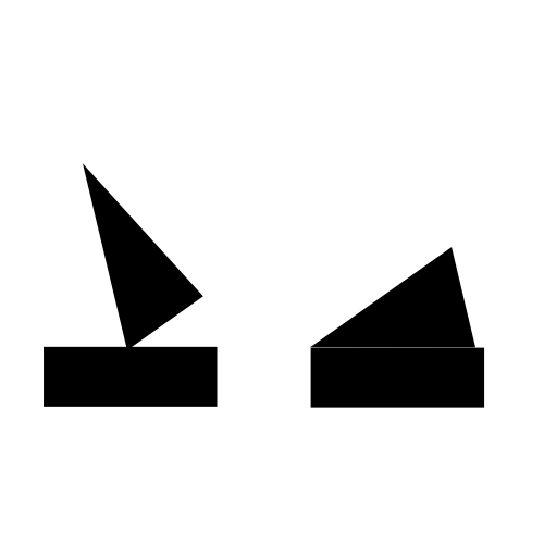
In the following section, we will use a example to classify images of house and boat, both of which are constructed using rectangles and triangles as shown below:

Fig 1.

Prediction and Routing

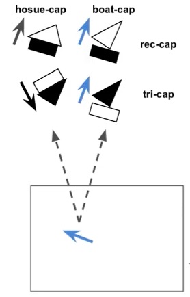
In the above boat and house example, we have two capsules to detect rectangle and triangle from the primary capsule respectively. The prediction contains two parts: probability of existence of certain element, and the direction. Suppose they will be feed into 2 capsules in the next layer: house-capsule and boat-capsule.

Assume that the rectangle capsule detect a rectangle rotated by 30 degrees, this feed into the next layer will result into house-capsule detecting a house rotated by 30 degrees. Similar for boat-capsule, where a boat rotated by 30 degrees will be detected in the next layer. Mathematically speaking, this can be written as: [math]\displaystyle{ \hat{u}_{ij} = W_{ij} u_i }[/math] where [math]\displaystyle{ u_i }[/math] is the own activation function of this capsule and [math]\displaystyle{ W_{ij} }[/math] is a transformation matrix being developed during training process.

Then look at the prediction from triangle capsule, which provides a different result in house-capsule and boat-capsule.

Fig 2.

Now we have four outputs in total, and we can see that the prediction in boat-capsule strongly agree to each other, which means we can reach the conclusion that the rectangle and triangle are parts of a boat; therefore, they should be routed to the boat-capsule. There is no need to send the output from primary capsule to any other capsules in the next layer, since this action will only add noise. This is the procedure called routing by agreement. Since only necessary outputs will be directed to the next layer, clearer signal will be received, and more accurate result will be produced. To implement routing by agreement, a clustering technique will be used and introduced in the next section.

Clustering and Updating

Fig 3.

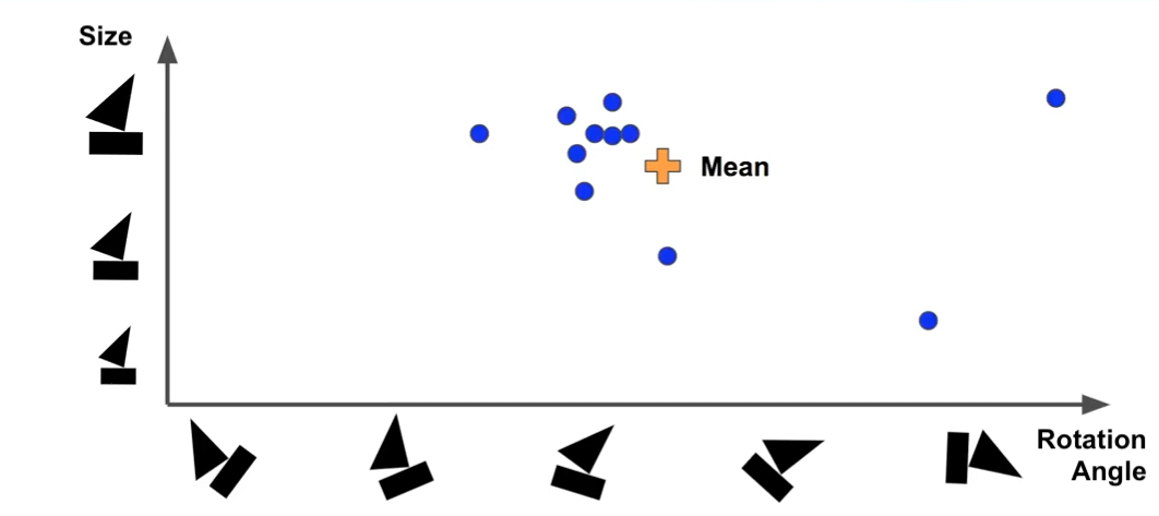
Suppose we represent capsules in the above graph, with x-axis representing rotation angle of the boat and y-axie representing the size. After find out the mean of data, we need to measure the distance between mean and prediction points on the graph by applying Euclidean distance or scalar product. The purpose of this step is to understand how much each prediction vector agrees with the mean, so that the weights of predicted vector can be output and updated. If the prediction matches mean well (i.e. the distance is small), more weights will be assigned to it. After getting the new weights, a weighted-mean will be computed, and it will be used to compute the distance again, and updated iteratively until reaches a steady state.

Mathematically speaking, the procedure starts with 0 weights for all prediction initially. Round1:

 bij = 0 for all i and j
 ci = softmax(bi)
 sj = weighted sum of predictions of each capsule in the next layer  
 vj = squash(sj), which will be the actual outputs of the next layers

After round1, we will update all [math]\displaystyle{ b_{ij} }[/math] as: [math]\displaystyle{ b_{ij} += \hat{u}_j * v_{ji} }[/math], then perform the next steps iteratively.