copyofstat341
General Methods
Since the Multiplicative Congruential Method can only be used for the uniform distribution, other methods must be developed in order to generate pseudo random numbers from other distributions.
Inverse Transform Method
This method uses the fact that when a random sample from the uniform distribution is applied to the inverse of a cumulative density function (cdf) of some distribution, the result is a random sample of that distribution. This is shown by this theorem:
Theorem:
If [math]\displaystyle{ U \sim~ \mathrm{Unif}[0, 1] }[/math] is a random variable and [math]\displaystyle{ X = F^{-1}(U) }[/math], where F is continuous, monotonic, and is the cumulative density function (cdf) for some distribution, then the distribution of the random variable X is given by F(X).
Proof:
Recall that, if f is the pdf corresponding to F where f is defined as 0 outside of its domain, then,
- [math]\displaystyle{ F(x) = P(X \leq x) = \int_{-\infty}^x f(x) }[/math]
- [math]\displaystyle{ \int_1^{\infty} \frac{x^k}{x^2} dx }[/math]
So F is monotonically increasing, since the probability that X is less than a greater number must be greater than the probability that X is less than a lesser number.
Note also that in the uniform distribution on [0, 1], we have for all a within [0, 1], [math]\displaystyle{ P(U \leq a) = a }[/math].
So,
- [math]\displaystyle{ \begin{align} P(F^{-1}(U) \leq x) &{}= P(F(F^{-1}(U)) \leq F(x)) \\ &{}= P(U \leq F(x)) \\ &{}= F(x) \end{align} }[/math]
Completing the proof.
Procedure (Continuous Case)
This method then gives us the following procedure for finding pseudo random numbers from a continuous distribution:
- Step 1: Draw [math]\displaystyle{ U \sim~ Unif [0, 1] }[/math].
- Step 2: Compute [math]\displaystyle{ X = F^{-1}(U) }[/math].
Example:
Suppose we want to draw a sample from [math]\displaystyle{ f(x) = \lambda e^{-\lambda x} }[/math] where [math]\displaystyle{ x \gt 0 }[/math] (the exponential distribution).
We need to first find [math]\displaystyle{ F(x) }[/math] and then its inverse, [math]\displaystyle{ F^{-1} }[/math].
- [math]\displaystyle{ F(x) = \int^x_0 \theta e^{-\theta u} du = 1 - e^{-\theta x} }[/math]
- [math]\displaystyle{ F^{-1}(x) = \frac{-\log(1-y)}{\theta} = \frac{-\log(u)}{\theta} }[/math]
Now we can generate our random sample [math]\displaystyle{ u_1\dots u_n }[/math] from [math]\displaystyle{ F(x) }[/math] by:
- [math]\displaystyle{ 1)\ u_i \sim Unif[0, 1] }[/math]
- [math]\displaystyle{ 2)\ x_i = \frac{-\log(u_i)}{\theta} }[/math]
The [math]\displaystyle{ x_i }[/math] are now a random sample from [math]\displaystyle{ f(x) }[/math].
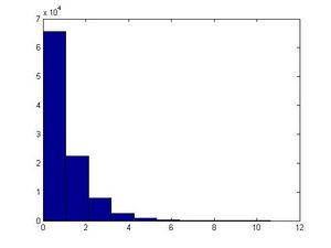
This example can be illustrated in Matlab using the code below. Generate [math]\displaystyle{ u_i }[/math], calculate [math]\displaystyle{ x_i }[/math] using the above formula and letting [math]\displaystyle{ \theta=1 }[/math], plot the histogram of [math]\displaystyle{ x_i }[/math]'s for [math]\displaystyle{ i=1,...,100,000 }[/math].
u=rand(1,100000);
x=-log(1-u)/1;
hist(x)

The major problem with this approach is that we have to find [math]\displaystyle{ F^{-1} }[/math] and for many distributions it is too difficult (or impossible) to find the inverse of [math]\displaystyle{ F(x) }[/math]. Further, for some distributions it is not even possible to find [math]\displaystyle{ F(x) }[/math] (i.e. a closed form expression for the distribution function, or otherwise; even if the closed form expression exists, it's usually difficult to find [math]\displaystyle{ F^{-1} }[/math]).
Procedure (Discrete Case)
The above method can be easily adapted to work on discrete distributions as well.
In general in the discrete case, we have [math]\displaystyle{ x_0, \dots , x_n }[/math] where:
- [math]\displaystyle{ \begin{align}P(X = x_i) &{}= p_i \end{align} }[/math]
- [math]\displaystyle{ x_0 \leq x_1 \leq x_2 \dots \leq x_n }[/math]
- [math]\displaystyle{ \sum p_i = 1 }[/math]
Thus we can define the following method to find pseudo random numbers in the discrete case (note that the less-than signs from class have been changed to less-than-or-equal-to signs by me, since otherwise the case of [math]\displaystyle{ U = 1 }[/math] is missed):
- Step 1: Draw [math]\displaystyle{ U~ \sim~ Unif [0,1] }[/math].
- Step 2:
- If [math]\displaystyle{ U \lt p_0 }[/math], return [math]\displaystyle{ X = x_0 }[/math]
- If [math]\displaystyle{ p_0 \leq U \lt p_0 + p_1 }[/math], return [math]\displaystyle{ X = x_1 }[/math]
- ...
- In general, if [math]\displaystyle{ p_0+ p_1 + \dots + p_{k-1} \leq U \lt p_0 + \dots + p_k }[/math], return [math]\displaystyle{ X = x_k }[/math]
Example (from class):
Suppose we have the following discrete distribution:
- [math]\displaystyle{ \begin{align} P(X = 0) &{}= 0.3 \\ P(X = 1) &{}= 0.2 \\ P(X = 2) &{}= 0.5 \end{align} }[/math]
The cumulative density function (cdf) for this distribution is then:
- [math]\displaystyle{ F(x) = \begin{cases} 0, & \text{if } x \lt 0 \\ 0.3, & \text{if } 0 \leq x \lt 1 \\ 0.5, & \text{if } 1 \leq x \lt 2 \\ 1, & \text{if } 2 \leq x \end{cases} }[/math]
Then we can generate numbers from this distribution like this, given [math]\displaystyle{ u_0, \dots, u_n }[/math] from [math]\displaystyle{ U \sim~ Unif[0, 1] }[/math]:
- [math]\displaystyle{ x_i = \begin{cases} 0, & \text{if } u_i \leq 0.3 \\ 1, & \text{if } 0.3 \lt u_i \leq 0.5 \\ 2, & \text{if } 0.5 \lt u_i \leq 1 \end{cases} }[/math]
This example can be illustrated in Matlab using the code below:
p=[0.3,0.2,0.5];
for i=1:1000;
  u=rand;
  if u <= p(1)
    x(i)=0;
  elseif u < sum(p(1,2))
    x(i)=1;
  else
    x(i)=2;
  end
end