Attend and Predict: Understanding Gene Regulation by Selective Attention on Chromatin
This page contains a summary of the paper "Attend and Predict: Understanding Gene Regulation by Selective Attention on Chromatin." by Singh, Ritambhara, et al. It was published at the Advances in Neural Information Processing Systems (NIPS) in 2017. The code for this paper is shared here[1].
Background
Gene regulation is the process of controlling which genes in a cell's DNA are turned 'on' (expressed) or 'off' (not expressed). By this process, a functional product such as a protein is created. Even though all the cells of a multicellular organism (e.g., humans) contain the same DNA, different types of cells in that organism may express very different sets of genes. As a result, each cell types have distinct functionality. In other words how a cell operates depends upon the genes expressed in that cell. Many factors including ‘Chromatin modification marks’ influence which genes are abundant in that cell.
The function of chromatin is to efficiently wraps DNA around bead-like structures of histones into a condensed volume to fit into the nucleus of a cell, and protect the DNA structure and sequence during cell division and replication. Different chemical modifications in the histones of the chromatin, known as histone marks, change spatial arrangement of the condensed DNA structure. Which in turn affects the gene’s expression of the histone mark’s neighboring region. Histone marks can promote (obstruct) the gene to be turned on by making the gene region accessible (restricted). This section of the DNA, where histone marks can potentially have an impact, is known as DNA flanking region or ‘gene region’ which is considered to cover 10k base pair centered at the transcription start site (TSS) (i.e., a 5k base pair in each direction). Unlike genetic mutations, histone modifications are reversible [1]. Therefore, understanding the influence of histone marks in determining gene regulation can assist in developing drugs for genetic diseases.
Introduction
Revolution in genomic technologies now enables us to profile genome-wide chromatin mark signals. Therefore, biologists can now measure gene expressions and chromatin signals of the ‘gene region’ for different cell types covering whole human genome. The Roadmap Epigenome Project (REMC, publicly available) [2] recently released 2,804 genome-wide datasets of 100 separate “normal” (not diseased) human cells/tissues, among which 166 datasets are gene expression reads and the rest are signal reads of various histone marks. The goal is to understand which histone marks are the most important and how they interact together in gene regulation for each cell type.
Signal reads for histone marks are high-dimensional and spatially structured. Influence of a histone modification mark can be anywhere in the gene region (covering 10k base pairs centered around the Transcription Start Site of each gene). It is important to understand how the impact of the mark on gene expression varies over the gene region. In other words, how histone signals over the gene region impacts the gene expression. There are different types of histone marks in human chromatin that can have an influence on gene regulation. Researchers have found five standard histone proteins. These five histone proteins can be altered in different combinations with different chemical modifications resulting in a large number of distinct histone modification marks. Different histone modification marks can act as a module to interact with each other and influence the gene expression.
This paper proposes an attention-based deep learning model to find how this chromatin factors/ histone modification marks contributes to the gene expression of a particular cell. AttentiveChrome[3] utilizes a hierarchy of multiple LSTM to discover interactions between signals of each histone marks, and learn dependencies among the marks on expressing a gene. The authors included two levels of soft attention mechanism, (1) to attend to the most relevant signals of a histone mark, and (2) to attend to the important marks and their interactions. In this context, attention refers to weighting the importance of different items differently.
Main Contributions
The contributions of this work can be summarized as follows:
- More accurate predictions than the state-of-the-art baselines. This is measured using datasets from REMC on 56 different cell types.
- Better interpretation than the state-of-the-art methods for visualizing deep learning model. They compute the correlation of the attention scores of the model with the mark signal from REMC.
- Like the application of attention models previously in indirectly hinting the parts of the input that the model deemed important, AttentiveChrome can too explain it's decisions by hinting at “what” and “where” it has focused.
- This is the first time that the attention based deep learning approach is applied to a problem in molecular biology.
- Ability to deal with highly modular inputs
Previous Works
Machine learning algorithms to classify gene expression from histone modification signals have been surveyed by [15]. These algorithms vary from linear regression, support vector machine, and random forests to rule-based learning, and CNNs. To accommodate the spatially structured, high dimensional input data (histone modification signals) these studies applied different feature selection strategies. The preceding research study, DeepChrome [4], by the authors incorporated the best position selection strategy. The positions that are highly correlated to the gene expression are considered as the best positions. This model can learn the relationship between the histone marks. This CNN based DeepChrome model outperforms all the previous works. However, these approaches either (1) failed to model the spatial dependencies among the marks, or (2) required additional feature analysis. Only AttentiveChrome is reported to satisfy all of the eight desirable metrics of a model.
AttentiveChrome: Model Formulation
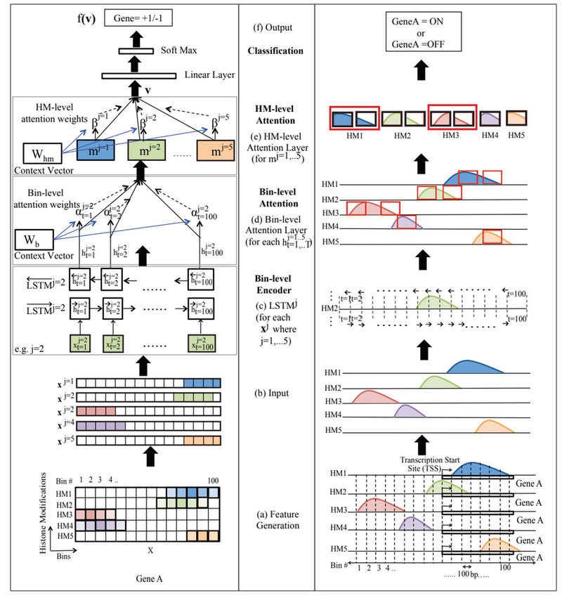
The authors proposed an end-to-end architecture which has the ability to simultaneously attend and predict. This method incorporates recurrent neural networks (RNN) composed of LSTM units to model the sequential spatial dependencies of the gene regions and predict gene expression level from The embedding vector, [math]\displaystyle{ h_t }[/math], output of an LSTM module encodes the learned representation of the feature dependencies from the time step 0 to [math]\displaystyle{ t }[/math]. For this task, each bin position of the gene region is considered as a time step.
The proposed AttentiveChrome framework contains following 5 important modules:
- Bin-level LSTM encoder encoding the bin positions of the gene region (one for each HM mark)
- Bin-level [math]\displaystyle{ \alpha }[/math]-Attention across all bin positions (one for each HM mark)
- HM-level LSTM encoder (one encoder encoding all HM marks)
- HM-level [math]\displaystyle{ \beta }[/math]-Attention among all HM marks (one)
- The final classification module
Figure 1 (Supplementary Figure 2) presents an overview of the proposed AttentiveChrome framework.
Input and Output
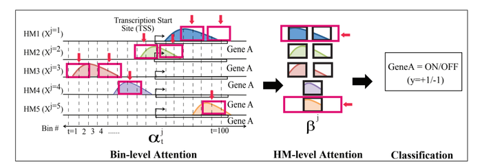
Each dataset contains the gene expression labels and the histone signal reads for one specific cell type. The authors evaluated AttentiveChrome on 56 different cell types. For each mark, we have a feature/input vector containing the signals reads surrounding the gene’s TSS position (gene region) for the histone mark. The label of this input vector denotes the gene expression of the specific gene. This study considers binary labeling where [math]\displaystyle{ +1 }[/math] denotes gene is expressed (on) and [math]\displaystyle{ -1 }[/math] denotes that the gene is not expressed (off). Each histone marks will have one feature vector for each gene. The authors integrates the feature inputs and outputs of their previous work DeepChrome [4] into this research. The input feature is represented by a matrix [math]\displaystyle{ \textbf{X} }[/math] of size [math]\displaystyle{ M \times T }[/math], where [math]\displaystyle{ M }[/math] is the number of HM marks considered in the input, and [math]\displaystyle{ T }[/math] is the number of bin positions taken into account to represent the gene region. The [math]\displaystyle{ j^{th} }[/math] row of the vector [math]\displaystyle{ \textbf{X} }[/math], [math]\displaystyle{ x_j }[/math], represents sequentially structured signals from the [math]\displaystyle{ j^{th} }[/math] HM mark, where [math]\displaystyle{ j\in \{1, \cdots, M\} }[/math]. Therefore, [math]\displaystyle{ x_j^t }[/math], in the matrix [math]\displaystyle{ \textbf{X} }[/math] represents the value from the [math]\displaystyle{ t^{th} }[/math] bin belonging to the [math]\displaystyle{ j^{th} }[/math] HM mark, where [math]\displaystyle{ t\in \{1, \cdots, T\} }[/math]. If the training set contains [math]\displaystyle{ N_{tr} }[/math] labeled pairs, the [math]\displaystyle{ n^{th} }[/math] is specified as [math]\displaystyle{ ( X^n, y^n) }[/math], where [math]\displaystyle{ X^n }[/math] is a matrix of size [math]\displaystyle{ M \times T }[/math] and [math]\displaystyle{ y^n \in \{ -1, +1 \} }[/math] is the binary label, and [math]\displaystyle{ n \in \{ 1, \cdots, N_{tr} \} }[/math].
Figure 2 (also refer to Figure 1 (a), and 1(b) for better understanding) exhibits the input feature, and the output of AttentiveChrome for a particular gene (one sample).
Bin-Level Encoder (one LSTM for each HM)
The sequentially ordered elements (each element actually is a bin position) of the gene region of [math]\displaystyle{ n^{th} }[/math] gene is represented by the [math]\displaystyle{ j_{th} }[/math] row vector [math]\displaystyle{ x^j }[/math]. The authors considered each bin position as a time step for LSTM. This study incorporates bidirectional LSTM to model the overall dependencies among a total of [math]\displaystyle{ T }[/math] bin positions in the gene region. The bidirectional LSTM contains two LSTMs
- A forward LSTM, [math]\displaystyle{ \overrightarrow{LSTM_j} }[/math], to model [math]\displaystyle{ x^j }[/math] from [math]\displaystyle{ x_1^j }[/math] to [math]\displaystyle{ x_T^j }[/math], which outputs the embedding vector [math]\displaystyle{ \overrightarrow{h^t_j} }[/math], of size [math]\displaystyle{ d }[/math] for each bin [math]\displaystyle{ t }[/math]
- A reverse LSTM, [math]\displaystyle{ \overleftarrow{LSTM_j} }[/math], to model [math]\displaystyle{ x^j }[/math] from [math]\displaystyle{ x_T^j }[/math] to [math]\displaystyle{ x_1^j }[/math], which outputs the embedding vector [math]\displaystyle{ \overleftarrow{h^j_t} }[/math], of size [math]\displaystyle{ d }[/math] for each bin [math]\displaystyle{ t }[/math]
The final output of this layer, embedding vector at [math]\displaystyle{ t^{th} }[/math] bin for the [math]\displaystyle{ j^{th} }[/math] HM, [math]\displaystyle{ h^j_t }[/math], of size [math]\displaystyle{ d }[/math], is obtained by concatenating the two vectors from the both directions. Therefore, [math]\displaystyle{ h^j_t = [ \overrightarrow{h^j_t}, \overleftarrow{h^j_t}] }[/math]. By pairing these LSTM-based HM encoders with the final classification, embedding each HM mark by drawing out the dependencies among bins can be learned by these pairs.Figure 1 (c) illustrates the module for [math]\displaystyle{ j=2 }[/math].
Bin-Level [math]\displaystyle{ \alpha }[/math]-attention
Each bin contributes differently in the encoding of the entire [math]\displaystyle{ j^{th} }[/math] mark. To automatically and adaptively highlight the most important bins for prediction, a soft attention weight vector [math]\displaystyle{ \alpha^j }[/math] of size [math]\displaystyle{ T }[/math] is learned for each [math]\displaystyle{ j }[/math]. To calculated the soft weight [math]\displaystyle{ \alpha^j_t }[/math], for each [math]\displaystyle{ t }[/math], the embedding vectors [math]\displaystyle{ \{h^j_1, \cdots, h^j_t \} }[/math] of all the bins are utilized. The following equation is used:
[math]\displaystyle{ \alpha^j_t = \frac{exp(\textbf{W}_b h^j_t)}{\sum_{i=1}^T{exp(\textbf{W}_b h^j_i)}} }[/math]
[math]\displaystyle{ \alpha^j_t }[/math] is a scalar and is computed by all bins’ embedding vectors [math]\displaystyle{ h^j }[/math]. The parameter [math]\displaystyle{ W_b }[/math] is initialized randomly, and learned alongside during the process with the other model parameters. Therefore, once we have importance weight of each bin position, the [math]\displaystyle{ j^{th} }[/math] HM mark can be represented by [math]\displaystyle{ m^j = \sum_{t=1}^T{\alpha^j_t \times h^j_t} }[/math]. Here, [math]\displaystyle{ h^j_t }[/math] is the embedding vector and [math]\displaystyle{ \alpha^t_j }[/math] is the importance weight of the [math]\displaystyle{ t^{th} }[/math] bin in the representation of the [math]\displaystyle{ j^{th} }[/math] HM mark. Intuitively [math]\displaystyle{ \textbf{W}_b }[/math] will learn the cell type. Figure 1(d) shows this module for [math]\displaystyle{ HM_2 }[/math].
HM-level Encoder (one LSTM)
Studies observed that HMs work cooperatively to provoke or subdue gene expression [5]. The HM-level encoder (not in the fFgure 1) utilizes one bidirectional LSTM to capture this relationship between the HMs. To formulate the sequential dependency a random sequence is imagined as the authors did not find influence of any specific ordering of the HMs. The representation [math]\displaystyle{ m_j }[/math]of the [math]\displaystyle{ j^{th} }[/math] HM, [math]\displaystyle{ HM_j }[/math], which is calculated from the bin-level attention layer, is the input of this step. This set based encoder outputs an embedding vector [math]\displaystyle{ s^j }[/math] of size [math]\displaystyle{ d’ }[/math], which is the encoding for the [math]\displaystyle{ j^{th} }[/math] HM.
[math]\displaystyle{ s^j = [ \overrightarrow{LSTM_s}(m_j), \overleftarrow{LSTM_s}(m_j) ] }[/math]
The dependencies between [math]\displaystyle{ j^{th} }[/math] HM and the other HM marks are encoded in [math]\displaystyle{ s^j }[/math], whereas [math]\displaystyle{ m^j }[/math] from the previous step encodes the bin dependencies of the [math]\displaystyle{ j^{th} }[/math] HM.
HM-Level [math]\displaystyle{ \beta }[/math]-attention
This second soft attention level (Figure 1(e)) finds the important HM marks for classifying a gene’s expression by learning the importance weights, [math]\displaystyle{ \beta_j }[/math], for each [math]\displaystyle{ HM_j }[/math], where [math]\displaystyle{ j \in \{ 1, \cdots, M \} }[/math]. The equation is
[math]\displaystyle{ \beta^j = \frac{exp(\textbf{W}_s s^j)}{\sum_{i=1}^M{exp(\textbf{W}_s s^j)}} }[/math]
The HM-level context parameter [math]\displaystyle{ \textbf{W}_s }[/math] is trained jointly in the process. Intuitively [math]\displaystyle{ \textbf{W}_s }[/math] learns how the HMs are significant for a cell type. Finally the entire gene region is encoded in a hidden representation [math]\displaystyle{ \textbf{v} }[/math], using the weighted sum of the embedding of all HM marks.
[math]\displaystyle{ \textbf{v} = \sum_{j=1}^MT{\beta^j \times s^j} }[/math]
End-to-end training
The embedding vector [math]\displaystyle{ \textbf{v} }[/math] is fed to a simple classification module, [math]\displaystyle{ f(\textbf{v}) = }[/math]softmax[math]\displaystyle{ (\textbf{W}_c\textbf{v}+b_c) }[/math], where [math]\displaystyle{ \textbf{W}_c }[/math], and [math]\displaystyle{ b_c }[/math] are learnable parameters. The output is the probability of gene expression being high (expressed) or low (suppressed). The whole model including the attention modules is differentiable. Thus backpropagation can perform end-to-end learning trivially. The negative log-likelihood loss function is minimized in the learning.
Experimental Settings
This work makes use of the REMC dataset. AttentiveChrome is evaluated on 56 different cell types. Similar to DeepChrome, this study considered the following five core HM marks ([math]\displaystyle{ M=5 }[/math]). Because these selected marks are uniformly profiled across all 56 cell types in the REMC study.
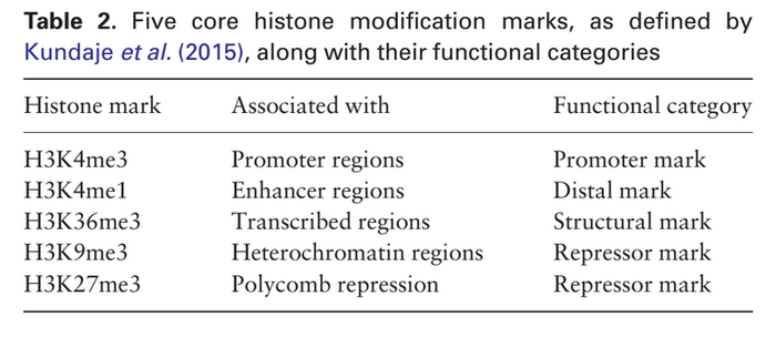
For a gene region 10k base pairs centred at the TSS site (5k bp in each direction) are taken into account. These 10k base pairs are divided into 100 bins, each bin consisting of [math]\displaystyle{ T=100 }[/math] continuous bp). Therefore, for each gene in a particular cell type, the input matrix will be of size [math]\displaystyle{ 5 \times 100 }[/math]. The gene expression labels are normalized and discretized to represent binary labelling. The sample dataset is divided into three equal sized folds for training, validation, and testing.
Model Variations and Two Baselines
To evaluate the performance of the proposed model the authors considered RNN method (direct LSTM without any attention), and their prior work DeepChrome as baselines. The results obtained from multiple variations of the AttentiveChrome model are compared with the baselines. The authors considered five variant of AttentiveChrome during performance evaluation. The variants are:
- LSTM-Attn: one LSTM with attention on the input matrix (does not consider the modular nature of HM marks)
- CNN-Attn: DeepChrome [4] with one attention mechanism incorporated.
- LSTM-[math]\displaystyle{ \alpha , \beta }[/math]: the proposed architecture.
- CNN-[math]\displaystyle{ \alpha , \beta }[/math]: LSTM module of the proposed architecture replaced with CNN. This variation includes two attention mechanisms. First attention mechanism contains one [math]\displaystyle{ \alpha }[/math]-attention on top of a CNN module per HM mark. And, the second -[math]\displaystyle{ \beta }[/math]- attention mechanism is used to combine HMs.
- LSTM-[math]\displaystyle{ \alpha }[/math]: one LSTM and [math]\displaystyle{ \alpha }[/math]-attention per HM mark.
Hyperparameters
For all the variants of AttentiveChrome the bin-level LSTM embedding size [math]\displaystyle{ d }[/math] is set to 32, and the HM-level LSTM embedding size [math]\displaystyle{ d’ }[/math] is set to 16. Because of bidirectional LSTM, the size of the embedding vector [math]\displaystyle{ h_t }[/math], and [math]\displaystyle{ m_j }[/math] will be 64, and 32 respectively. Size of the context vectors are set accordingly.
Performance Evaluation
AUC Scores
This study summarizes AUC scores across all 56 cell types on the test set to compare the methods.
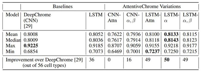
Overall the LSTM-attention models perform better than the DeepChrome (CNN-based) and LSTM baselines. The authors argue that the proposed AttentiveChrome model is a good choice because of its interpretability, even though the performance improvement from DeepChrome is insignificant.
Evaluation of Attention Scores for Interpretation
To understand if the model is focusing on the right regions, the authors make use of additional study results from REMC database. To validate the bin attention,signal data of a new histone mark, H3K27ac, referred to as [math]\displaystyle{ H_{active} }[/math] in this article, from REMC database is utilized. This particular histone mark is known to mark active region when the gene is expressed (ON). Genome-wide read of this HM mark is available for three important cell types: stem cell (H1-hESC), blood cell (GM12878), and leukemia cell (K562). This particular HM mark is used to analyze the visualization results only and not applied in the learning phase. The authors discussed performance of both the attention mechanisms in this section.
Correlation of Importance Weight of [math]\displaystyle{ H_{prom} }[/math] with [math]\displaystyle{ H_{active} }[/math]
Average read count of [math]\displaystyle{ H_{active} }[/math] across all 100 bins for all the active genes (ON or labeled as [math]\displaystyle{ +1 }[/math]) in the three selected cell types is calculated. The proposed AttentiveChrome and LSTM-[math]\displaystyle{ \alpha }[/math] methods are compared with two widely used visualization techniques, (1) class based, and (2) saliency map applied on the baseline DeepChrome model (CNN-based prior work). Using these visualization methods, the authors calculate the importance weights for [math]\displaystyle{ H_{prom} }[/math] (promoter HM mark used in training) across the 100 bins. The Pearson Correlation score between these importance weights and the read count of the [math]\displaystyle{ H_{active} }[/math] (HM mark for validation) across the same 100 bins is computed. The [math]\displaystyle{ H_{active} }[/math] read counts indicates the actual active regions of those cells.

The results indicate that the proposed models consistently gained highest correlation with [math]\displaystyle{ H_{active} }[/math] for all three cell types. Thus, the proposed method is successful to capture the important signals.
Visualization of Attention Weight of bins for each HM of a specific cell type GM12878
To visualize bin level attention weights, the authors plotted the average bin-level attention weights for each HM for a specific cell type GM12878 (blood cell) for expressed (ON) genes and suppressed (OFF) genes separately.
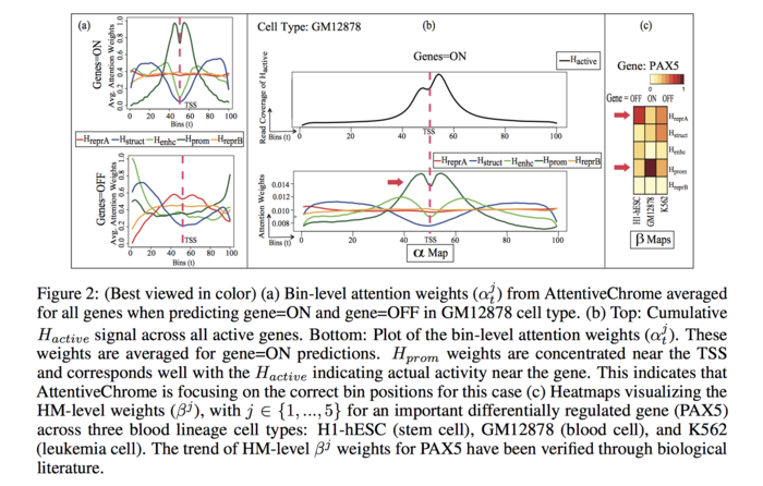
For the “ON” genes, the attention profiles are well defined for the HM marks, [math]\displaystyle{ H_{prom} }[/math], [math]\displaystyle{ H_{enhc} }[/math], [math]\displaystyle{ H_{struct} }[/math]. On the other hand, the weights are low for [math]\displaystyle{ H_{reprA} }[/math] and [math]\displaystyle{ H_{reprB} }[/math]. The average trend reverses for the “OFF” genes, where the repressor HM marks have more influence than the [math]\displaystyle{ H_{prom} }[/math], [math]\displaystyle{ H_{enhc} }[/math], [math]\displaystyle{ H_{struct} }[/math]. This observation agrees with the biologist finding that [math]\displaystyle{ H_{prom} }[/math], [math]\displaystyle{ H_{enhc} }[/math], [math]\displaystyle{ H_{struct} }[/math] marks stimulates gene activation and, [math]\displaystyle{ H_{reprA} }[/math] and [math]\displaystyle{ H_{reprB} }[/math] mark restrains the genes.
Attention Weight of bins with [math]\displaystyle{ H_{active} }[/math]
The average read counts of [math]\displaystyle{ H_{active} }[/math] for the same 100 bins across all the active (ON) genes for the cell type GM12878 is plotted (FIGURE 2(b)). Besides, for AttentiveChrome the plot of bin-level attention weights of averaged over all the genes that are PREDICTED ON for GM12878 is also provided. The plots exhibit that the [math]\displaystyle{ H_{prom} }[/math] profile is similar to [math]\displaystyle{ H_{active} }[/math].
Visualization of HM-level Attention Weight for Gene PAX5
To visualize HM-level attention weight the authors produces a heatmap for a differentially regulated gene, PAX5, for the three aforementioned cell types. The heatmap is presented in FIGURE 2(c). PAX5 plays significant role in gene regulation when stem cells convert to blood cells. This gene is OFF in stem cells (H1-hESC), however it becomes activated when the stem cell is transformed into blood cell (GM12878). The [math]\displaystyle{ \beta_j }[/math] weight for [math]\displaystyle{ H_{repr} }[/math] is high when the gene is OFF in H1-hESC, and the weight decreases when the gene is ON in GM12878. On the contrary, for [math]\displaystyle{ H_{prom} }[/math] mark the [math]\displaystyle{ \beta_j }[/math] weight increases from H1-hESC to GM12878 as the gene becomes activated. This information extracted by the deep learning model is also supported by biological literature [16].
Related Works/Studies
In the last few years, deep learning models obtained models obtained unprecedented success in diverse research fields. Though as not rapidly as other fields, deep learning based algorithms are gaining popularity among bioinformaticians.
Attention-based Deep Models
The idea of attention technique in deep learning is adapted from the human visual perception system. Humans tend to focus over some parts more than the others while perceiving a scene. This mechanism augmented with deep neural networks achieved an excellent outcome in several research topics, such as machine translation. Various types of attention models e.g., soft [6], or location-aware [7], or hard [8, 9] attentions have been proposed in the literature. In the soft attention model, a soft weight vector is calculated for the overall feature vectors. The extent of the weight is correlated with the degree of importance of the feature in the prediction. In practice, RNN is often used to help implement such models.
Visualization and Apprehension of Deep Models
Prior studies mostly focused on interpreting convolutional neural networks (CNN) for image classification. Deconvulation approaches [10] attempt to map hidden layer representations back to an input space. Saliency maps [11, 12], attempt to use taylor expansion to approximate the network, and identify the most relevant input features. Class optimization [12] based visualization techniques attempt to find the best example member of each class. Some recent research works [13, 14] tried to understand recurrent neural networks (RNN) for text-based problems. By looking into the features the model attends to, we can interpret the output of a deep model.
Deep Learning in Bioinformatics
Deep learning is also getting popular in bioinformatics fields because it is able to extract meaningful representations from datasets. Scholars use deep learning to model protein sequences and DNA sequences and predicting gene expressions.
Previous model for gene expression predictions
There were multiple machine learning models had been used to predict gene expressions, such as linear regression and support vector machines. The strategies included using signal averaging across all relevant positions and selecting input signals at positions where was highly correlated to target gene expression and then use CNN to learn combinatorial interactions among histone modification marks.
Conclusion
The paper has introduced an attention-based approach called "AttentiveChrome" that deals with both understanding and prediction with several advantages on previous architectures including higher accuracy from state-of-the-art baselines, clearer interpretation than saliency map, which allows them to view what the model ‘sees’ during prediction prediction, and class optimization. Another advantage of this approach is that it can model modular feature inputs which are sequentially structured. Finally, according to the authors, this is the first implementation of deep attention to understand gene regulation. AttentiveChrome is claimed to be the first attention based model applied on a molecular biology dataset. The authors expect that through this deep attention mechanism the biologists can have a better understanding of epigenomic data. This model can handle understanding and prediction of hard to interpret biological data.
Critiques
This paper does not give a considerable algorithmic contribution. They have only used existing methods for this application. This deep learning based method is shown to perform better than simple machine learning models like linear regression and SVMs but this is considerably harder to implement and has many more hyperparameters to tune. The training time is considerably higher, especially because all the parameters are learned together. The dataset considered in the application here also seems to have only a limited number of samples for a study of high complexity. Model hyperparameters have been chosen randomly without any explanation of intuition for them. The authors have also not cited any relevant literature to understand where these numbers came from.
Discussion about attention scores for interpretation does not provide any clear definition or mention previous literature using them. Reference of literature about H3K27ac, and how its read counts represent active region of a cell should be included. No reasoning given for why only one specific cell type is used to visualize bin level attention weights. Example of some other real world problems where this model can be useful should be provided.
Moreover, this paper relies heavily on the intuition. Due to complicated structures, it must be challenging to provide algorithmic/theoretical justifications. This means that there is no proper guidence of how hyperparameters should be chosen or any kinds of treatment that the author performs on other data sets.
Additional Resources
Reference
[1] Andrew J Bannister and Tony Kouzarides. Regulation of chromatin by histone modifications. Cell Research, 21(3):381–395, 2011.
[2] Anshul Kundaje, Wouter Meuleman, Jason Ernst, Misha Bilenky, Angela Yen, Alireza Heravi-Moussavi, Pouya Kheradpour, Zhizhuo Zhang, Jianrong Wang, Michael J Ziller, et al. Integrative analysis of 111 reference human epigenomes. Nature, 518(7539):317–330, 2015.
[3] Singh, Ritambhara, et al. "Attend and Predict: Understanding Gene Regulation by Selective Attention on Chromatin." Advances in Neural Information Processing Systems. 2017.
[4] Ritambhara Singh, Jack Lanchantin, Gabriel Robins, and Yanjun Qi. Deepchrome: deep-learning for predicting gene expression from histone modifications. Bioinformatics, 32(17):i639–i648, 2016.
[5] Joanna Boros, Nausica Arnoult, Vincent Stroobant, Jean-François Collet, and Anabelle Decottignies. Polycomb repressive complex 2 and h3k27me3 cooperate with h3k9 methylation to maintain heterochromatin protein 1α at chromatin. Molecular and cellular biology, 34(19):3662–3674, 2014.
[6] Dzmitry Bahdanau, Kyunghyun Cho, and Yoshua Bengio. Neural machine translation by jointly learning to align and translate. arXiv preprint arXiv:1409.0473, 2014.
[7] Jan K Chorowski, Dzmitry Bahdanau, Dmitriy Serdyuk, Kyunghyun Cho, and Yoshua Bengio. Attention-based models for speech recognition. In C. Cortes, N. D. Lawrence, D. D. Lee, M. Sugiyama, and R. Garnett, editors, Advances in Neural Information Processing Systems 28, pages 577–585. Curran Associates, Inc., 2015.
[8] Minh-Thang Luong, Hieu Pham, and Christopher D. Manning. Effective approaches to attention-based neural machine translation. In Empirical Methods in Natural Language Processing (EMNLP), pages 1412–1421, Lisbon, Portugal, September 2015. Association for Computational Linguistics.
[9] Huijuan Xu and Kate Saenko. Ask, attend and answer: Exploring question-guided spatial attention for visual question answering. In ECCV, 2016.
[10] Matthew D Zeiler and Rob Fergus. Visualizing and understanding convolutional networks. In Computer Vision–ECCV 2014, pages 818–833. Springer, 2014.
[11] David Baehrens, Timon Schroeter, Stefan Harmeling, Motoaki Kawanabe, Katja Hansen, and Klaus-Robert MÞller. How to explain individual classification decisions. volume 11, pages 1803–1831, 2010.
[12] Karen Simonyan, Andrea Vedaldi, and Andrew Zisserman. Deep inside convolutional networks: Visualising image classification models and saliency maps. 2013.
[13] Andrej Karpathy, Justin Johnson, and Fei-Fei Li. Visualizing and understanding recurrent networks. 2015.
[14] Jiwei Li, Xinlei Chen, Eduard Hovy, and Dan Jurafsky. Visualizing and understanding neural models in nlp. 2015.
[15] Xianjun Dong and Zhiping Weng. The correlation between histone modifications and gene expression. Epigenomics, 5(2):113–116, 2013.
[16] Shane McManus, Anja Ebert, Giorgia Salvagiotto, Jasna Medvedovic, Qiong Sun, Ido Tamir, Markus Jaritz, Hiromi Tagoh, and Meinrad Busslinger. The transcription factor pax5 regulates its target genes by recruiting chromatin-modifying proteins in committed b cells. The EMBO journal, 30(12):2388–2404, 2011.